How to improve the state of the art in metocean measurement datasets
←
→
Page content transcription
If your browser does not render page correctly, please read the page content below
Wind Energ. Sci., 5, 285–308, 2020
https://doi.org/10.5194/wes-5-285-2020
© Author(s) 2020. This work is distributed under
the Creative Commons Attribution 4.0 License.

                 How to improve the state of the art in metocean
                            measurement datasets
                                         Erik Quaeghebeur and Michiel B. Zaaijer
            Wind Energy Section, Delft University of Technology, Kluyverweg 1, 2629 HS Delft, the Netherlands
                                Correspondence: Michiel B. Zaaijer (m.b.zaayer@tudelft.nl)

                                      Received: 17 July 2019 – Discussion started: 26 July 2019
                        Revised: 17 January 2020 – Accepted: 29 January 2020 – Published: 28 February 2020

       Abstract. We present an analysis of three datasets of 10 min metocean measurement statistics and our resulting
       recommendations to both producers and users of such datasets. Many of our recommendations are more gen-
       erally of interest to all numerical measurement data producers. The datasets analyzed originate from offshore
       meteorological masts installed to support offshore wind farm planning and design: the Dutch OWEZ and MMIJ
       and the German FINO1. Our analysis shows that such datasets contain issues that users should look out for
       and whose prevalence can be reduced by producers. We also present expressions to derive uncertainty and bias
       values for the statistics from information typically available about sample uncertainty. We also observe that the
       format in which the data are disseminated is sub-optimal from the users’ perspective and discuss how producers
       can create more immediately useful dataset files. Effectively, we advocate using an established binary format
       (HDF5 or netCDF4) instead of the typical text-based one (comma-separated values), as this allows for the in-
       clusion of relevant metadata and the creation of significantly smaller directly accessible dataset files. Next to
       informing producers of the advantages of these formats, we also provide concrete pointers to their effective use.
       Our conclusion is that datasets such as the ones we analyzed can be improved substantially in usefulness and
       convenience with limited effort.

1   Introduction                                                   although usually with some access and usage restrictions, es-
                                                                   pecially for commercial purposes.
The planning and design of offshore wind farms depends                We became interested in evaluating metocean measure-
heavily on the availability of representative meteorological       ment datasets after encountering a number of issues in a spe-
and ocean or “metocean” measurement data. For example,             cific dataset, both in data quality and in the dissemination
the wind resource (the wind speed and direction distribution)      format. (Our concrete purpose was to use it for wind farm
at the candidate farm location is used to estimate energy pro-     energy production estimation.) Discussion with other users
duction over the farm’s lifetime, and information about ocean      of such datasets showed that many found the typical dis-
waves is needed for wind turbine support structure design          semination approach, providing multiple files with comma-
and planning installation and maintenance.                         separated values, to be inconvenient or even a hindrance to
   The data are collected by instruments placed on fixed off-      their application. Most were not aware of the data quality is-
shore platforms, met masts, or measurement buoys deployed          sues we encountered, which can be categorized as faulty data,
in measurement campaigns. These campaigns are ordered by           missing documentation, inappropriate statistic selection, lim-
the project owner (a government or a farm developer) and           ited data quality information, and sub-optimal value encod-
set up and carried out by contractors (applied research in-        ing.
stitutes or companies). The dataset producer (one or more             Therefore, we performed a study of three commonly used
of the contractors) collects and processes the data generated      metocean datasets to answer essentially the following ques-
in these campaigns and provides them to dataset users. The         tions. (i) Are these issues commonly shared in metocean
datasets produced are often available publicly to these users,     datasets? (ii) How can the issues that are present be ad-

Published by Copernicus Publications on behalf of the European Academy of Wind Energy e.V.
286 E. Quaeghebeur and M. B. Zaaijer: How to improve the state of the art in metocean measurement datasets
dressed? This paper reports the results of that study. In brief, quantities measured, describe the dissemination approach,
(i) yes, there are shared issues, but, not unexpectedly, not all point to available documentation, and highlight some further
of them in all datasets, and (ii) dataset producers can address important aspects. We do this in full detail here for the first
the issues with a few non-burdensome additions to their cre- dataset, but for the other two we put aspects that are not sub-
ation practice. Next to providing arguments for and detailing stantively different in Appendix A1. We also provide a brief
these conclusions, this paper is meant to raise awareness of FAIRness analysis (Wilkinson et al., 2016) of the datasets in
the issues mentioned by giving concrete examples. Further- Appendix A1.3.
more, it provides dataset producers with concrete ideas about Common to all three datasets is that they can be down-
how to achieve substantial improvements with reasonable ef- loaded from a website, where some documentation is avail-
fort. able. But, also for all three, we needed to look up external
The users of the produced datasets are of course the farm sources and contact parties involved in the dataset creation
developers, but also the academic world, whose usage is not process to get a more complete view. The collected meta-
necessarily restricted to wind energy applications. The con- data are available as part of a separate bundle (Quaeghebeur,
text of our academic research is offshore wind energy, but 2020). It also includes details not mentioned in this paper,
the work we present here is relevant outside that area as well. such as the make and type of instruments and loggers.
Therefore, we treat all measured quantities on equal footing
and do not focus on wind and wave data. When our discus- 2.1.1 OWEZ – offshore wind farm Egmond aan Zee
sion goes beyond the analysis of the specific datasets we con-
sidered, it is also mostly independent of their metocean na- To gather data before and after construction of the offshore
ture but generally applies to any numerical time series data. wind farm Egmond aan Zee (OWEZ; “Offshore Windpark
We structure the paper into two main sections. We start Egmond aan Zee” in Dutch), a met mast was built on-site. Its
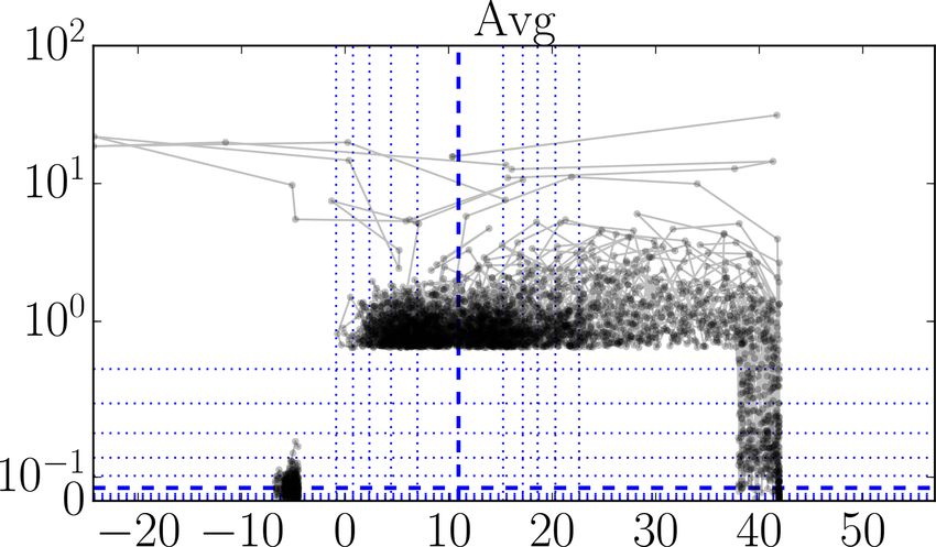
with an essentially descriptive Sect. 2, to give an overview location is 52◦ 360 22.900 N, 4◦ 230 22.700 E (WGS 84), which is
of the datasets we considered and to identify the issues we 15 km off the Dutch coast near the town Egmond aan Zee.
encountered. The original contributions here are our thor- The location is indicated in Fig. 1. The mast was erected in
ough description, in-depth analysis, and expressions of the 2003 and construction of the wind farm started in 2006. Data
uncertainties and bias in the statistics’ values that make up are publicly available for the period July 2005–December
the datasets. In this section we also mention options for ad- 2010. The instruments used and quantities measured and
dressing issues described, where it can be done compactly some of their characteristics are listed in Table 1.
and where we believe it adds value for dataset producers. In Due to an agreement between the Dutch government and
the instructional Sect. 3 we discuss how the format of these the OWEZ developer, data gathered and reports written in the
datasets can be improved and thereby disseminated more context of the wind farm’s construction have been made pub-
conveniently. This section includes an up-to-date evaluation licly available. This is done through a website where these
of binary dataset file format functionality. The recommen- materials can be downloaded (NoordzeeWind, 2019). The
dations to project owners, dataset producers, and users that metocean dataset can be downloaded as 66 separate monthly
follow from these analyses are collected at the end of this compressed Excel (xls) spreadsheet files. The total size is
paper (Sect. 4), preceding the overall conclusions (Sect. 5). almost 1 GB, or about 400 MB compressed. This represents
data points for 289 296 10 min intervals. The data in each file
are structured as follows:
2 The datasets and their analysis
– six date–time columns (year, month, day, hour, minutes,
We split our discussion of the datasets into two parts: first, seconds);
in Sect. 2.1, we present the three datasets in terms of context
and content, and then, in Sect. 2.2, we go over the issues we – 48 “channels” of five columns each: an integer identi-
encountered. fier “Channel” and four real-valued statistics, “Max”,
“Min”, “Mean”, and “StdDev”, with each channel cor-
2.1 A first look at the datasets responding to a specific measured quantity and location
on the mast.
All three datasets we consider come from measuring masts in
the North Sea and contain multiple multi-year 10 min statis- In the Excel files, the statistics’ values are encoded as 8 B
tics data, called “series”. These 10 min statistics are derived (byte) binary floating point numbers.
from higher-frequency measurements, called “signals”, of Information about the dataset, the met mast, and its con-
quantities measured by various instruments at various loca- text is available through the same website. In particular,
tions on the mast. The available statistics are the sample min- there is a user manual (Kouwenhoven, 2007) and several re-
imum, maximum, mean, and standard deviation. ports from which further information can be learned (e.g.,
For each dataset, we give a brief description of the mea- Curvers, 2007; Eecen and Branlard, 2008; Wagenaar and
surement site and setup, list the measurement period and Eecen, 2010a, b). Information about the instruments used and
Wind Energ. Sci., 5, 285–308, 2020 www.wind-energ-sci.net/5/285/2020/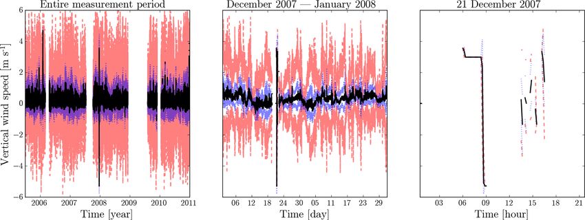
E. Quaeghebeur and M. B. Zaaijer: How to improve the state of the art in metocean measurement datasets                          287

Figure 1. A map with the location of the three offshore met masts from which data were analyzed: OWEZ, MMIJ, and FINO1.

in particular the measurement uncertainty had to be looked         datasets is that not all statistics are available for all signals.
up in specification sheets or obtained through personal com-       Also, it is free for academic research purposes but not for
munication with people involved in the project (see Ac-            commercial use, in contrast to the two other datasets. The
knowledgements).                                                   dataset is made available as a set of tab-separated-value (dat)
                                                                   files, and the statistics’ values are encoded in a decimal fixed-
2.1.2   MMIJ – measuring mast IJmuiden                             point format with up to two fractional digits (x...x.xx). For
                                                                   each quantity, a quality column is included next to the statis-
The second dataset, “MMIJ”, comes from a met mast in the           tics’ columns.
Dutch part of the North Sea. The location is indicated in
Fig. 1. Details can be found in Appendix A1.1.
                                                                   2.2     Dataset issues
  The exact set of signals differs of course from the OWEZ
dataset; we have given an overview in Table A1 in the ap-          We split the issues encountered in the datasets into five
pendix. The data were collected during the period 2011–            categories each discussed in their own section: faulty data
2016, a period of time comparable in length to OWEZ. The           (Sect. 2.2.1), documentation (Sect. 2.2.2), statistic selection
dataset is made available as a single semicolon-separated-         (Sect. 2.2.3), quality flags (Sect. 2.2.4), and value encoding
value (csv) file, and the statistics’ values are encoded in        and uncertainty propagation (Sect. 2.2.5).
a decimal fixed-point format with five fractional digits
(x...x.xxxxx).                                                     2.2.1    Faulty data
                                                                   It is not unusual that the measured signals (raw data) contain
2.1.3   FINO1 – research platform in the North Sea and
                                                                   faulty data. With this we mean data values that cannot corre-
        the Baltic Sea Nr. 1
                                                                   spond to the actual values or are very unlikely to correspond
The third dataset, “FINO1”, comes from a met mast in the           to them. The dataset producers deal with such faulty data,
German part of the North Sea. The location is indicated in         e.g., by flagging or removing it, when creating the datasets
Fig. 1. Details can be found in Appendix A1.2.                     of statistics series we study. Nevertheless, each of the three
   The exact set of signals again differs from the OWEZ            datasets presented above contained remaining faulty data.
dataset; we have given an overview in Table A2 in the ap-          We stumbled upon initial examples, but then systematically
pendix. The data investigated were collected during the pe-        looked for issues.
riod 2004–2016, so a period of time more than twice as long            To facilitate this systematic and partly automated investi-
as for the other two datasets. A difference with the other two     gation, we created binary file format versions of the datasets

www.wind-energ-sci.net/5/285/2020/                                                          Wind Energ. Sci., 5, 285–308, 2020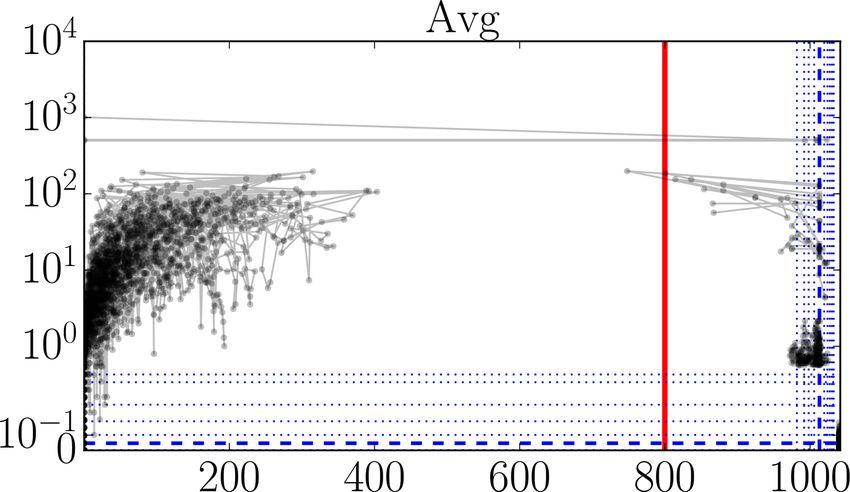
288                E. Quaeghebeur and M. B. Zaaijer: How to improve the state of the art in metocean measurement datasets

Table 1. An overview of the instruments and their locations on the OWEZ met mast (height in meters above mean sea level and boom
orientation), the quantity measured, measurement uncertainty, the measurement ranges, and the sampling frequencies.

  Instrument                         (No.)      Heightah        Orientationao         Quantity                   Unit           Uncertaintym      Rangem     Freq.m
                                                (m)                                                                            Abs.    Rel. (%)                (Hz)
  Accelerometer                      (1)        116             mast                  N–S accel.                 m s−2         0.01               −30–30        33
                                                                                      W–E accel.
  Cup anemometer                     (9)        all             all                   hor. wind sp.              m s−1         0.5                0–50            4
  Ultrasonic anemometer              (3)        all             NE                    hor. wind sp.              m s−1         0.01    1.5        0–60            4
                                                                                      vert. wind sp.
                                                                                      wind direction             ◦             2                  0–359           4
  Wind vane                          (9)        all             all                   wind direction             ◦             1.4                0–360
  Barometer                          (1)        20              mast                  atm. pressure              mbar          0.5                600–1100
  Thermometeri                       (3)        all             S                     ambient temp.              ◦C            0.1                −40–80
  Hygrometeri                        (3)        all             S                     rel. humidity              %             1                  0–100
  Precipitation sensor               (2)        70              NE, NW                precip. level              –
  Thermometer                        (1)        −3.8            mast                  water temp.                ◦C            0.15    0.1        −180–600
  Acoustic wave and                  (1)        −17             ?                     water temp.                ◦C            0.1                −4–40           1
  current profilerf                                                                   water level                m                                                4
                                                                                      wave height                m             0.01    1          −15–15          4
                                                                                      wave direction             ◦             2                  0–359           2
                                                                                      wave period                s                                0.5–50          2
                                                                                      current vel. 7 m           m s−1         0.005   1          −10–10          1
                                                                                      current vel. 11 m
                                                                                      current dir. 7 m           ◦                                0–359           1
                                                                                      current dir. 11 m
ah For height, “all” corresponds to 21, 70, and 116 m.
ao For orientation, “all” corresponds to NE, NW, and S or −60◦ , 60◦ , and 180◦ , respectively (north corresponding to 0◦ ).
i Thermometer and hygrometer are contained in a single package.
f The given sampling frequencies are upper bounds.
m Missing values are unknown.

(HDF5 format for OWEZ and netCDF4 format for MMIJ and                                                 even more. Zooming in further gives the right-hand plot,
FINO1) in which metadata such as range and possible values                                            which shows that many missing values surround the
can be stored alongside the data themselves. We discuss these                                         anomaly, further suggesting that the values still present
formats in more detail in Sect. 3. The automation essentially                                         here may not be reliable. (We do not know why the sur-
consisted of looping over all signals and statistics to detect                                        rounding values are missing.)
issues; further investigation was done manually.
   More concretely, our procedure was as follows.                                                2. We ran automated checks for values outside the instru-
                                                                                                    ment’s range for the series or for inconsistent sets of
  1. We performed interactive visual inspection of plots                                            statistics’ values. Let us clarify what inconsistent sets
     of the individual datasets, including zooming in on                                            of statistics’ values are. Statistic values imply bounds
     suspicious-looking parts. Figure 2 provides an example.                                        on the value of other statistics. If such a constraint is
     The plots should be read as follows: the mean value is                                         violated for some 10 min interval, the tuple of statis-
     given by the “inner” full (black) line; mean values plus                                       tics (minimum x̌, maximum x̂, mean x̄, standard devia-
     and minus 1 standard deviation are given by the “inter-                                        tion sx ) for that interval is inconsistent. For example, it
     mediate” dotted (blue) lines; minima and maxima are                                            should be the case that x̌ ≤ x̄ ≤ x̂; violations of this con-
     given by the “outer” dashed (red) lines. The plots in this                                     straint are present, e.g., in the FINO1 cup anemometer
     figure are snapshots of an interactive visualization pro-                                      wind speed data. Less obvious constraints involving the
     cedure: even though the lines overlap in the unzoomed                                          sample standard deviation also exist. We used 12 |x̂ − x̌|
     left-hand plot, an anomalous extreme mean value is visi-                                       as the general upper bound for the standard deviation,
     ble around the 2007–2008 year change. Zooming in a bit                                         given that the values lie in the interval [x̌, x̂] (Shiffler
     gives the middle plot, where the statistics start becom-                                       and Harsha, 1980). (Here x̌ and x̂ can be replaced by
     ing visually separated and where the anomaly stands out                                        range bounds in case the minimum and maximum statis-

Wind Energ. Sci., 5, 285–308, 2020                                                                                              www.wind-energ-sci.net/5/285/2020/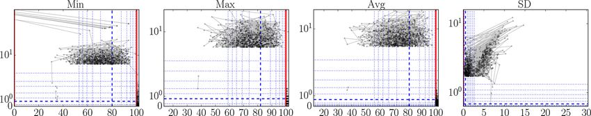
E. Quaeghebeur and M. B. Zaaijer: How to improve the state of the art in metocean measurement datasets                               289

Figure 2. An illustration of the visual inspection and zooming of plots. We present the OWEZ vertical wind speed data collected by the
ultrasonic anemometer at the NE-116 m location. (Mean in black; mean ± standard deviation in blue; minimum and maximum in red.)

Table 2. An overview of the (largest) range violations present in the FINO1 dataset. (Values rounded to three digits.)

                 Instrument                 Quantity            Unit       Statistic     Lowest      Instr. range   Highest
                 Cup anemometer             hor. wind sp.       m s−1      Minimum       0.0313      0.1–75
                                                                           Maximum                   0.1–75         1690
                 Ultrasonic anemometer      hor. wind sp.       m s−1      Maximum                   0–45           45.6
                                            wind direction      ◦          Average                   0–359          360
                 Wind vane                  wind direction      ◦          Maximum                   0–360          521
                                                                           Average                   0–360          366
                 Barometer                  atm. pressure       hPa        Average       0.00391     800–1060
                 Hygrometer                 rel. humidity       %          Average       0.0313      10–100         102
                 Precipitation sensor       precip. intensity   mA         Average       0.00195     4–20           45.3
                 Pyranometer                global radiation    W m−2      Average       −4.86       0–4000         145 000

     tics are not present in the dataset.) Any such incon-                     and contains metadata allows the code to be generic, i.e.,
     sistency is a serious issue, as it indicates a deficiency                 not variable-specific, and therefore compact.
     somewhere in the procedures for calculating statistics
     and their post-processing.                                            3. We did checks of the occurring values, for quantities
                                                                              with a discrete number of possible values. One exam-
     As an example, the range violations in the FINO1                         ple is the synoptic code “max” values from the MMIJ
     dataset gave the results listed in Table 2. Some range                   precipitation monitor. The check showed the following
     violations point to faulty data (e.g., cup anemometer–                   values to be present.
     hor. wind sp.–max, where the value exceeds the bound
                                                                               −998 −997           −953    −952     −950      −900 −176
     by more than an order of magnitude), but others sug-
     gest a need for more elaborate uncertainty analysis (e.g.,                 −16          0       51       53         55     58    59
     hygrometer–rel. humidity–avg., where the violating val-                       61      63        65       68         69     71    73
     ues probably correspond to the bounds) or more elab-                          75      77        87       88         89     90   108
     orate handling of the range bounds (e.g., wind vane–
     wind direction–max, where the upper bound could be                        Synoptic code values below 0 and above 99 do not ex-
     increased; also see Appendix A2.1).                                       ist (World Meteorological Organization, 2016, p. 356–
                                                                               358), so faulty data are present here. Only integer values
     The code producing the results of Table 2 is pub-                         are present here, but erroneous fractional values would
     licly available (Quaeghebeur, 2020). The fact that our                    also be detected. The code for performing this check is
     netCDF4 version of the dataset is (uniformly) structured                  publicly available (Quaeghebeur, 2020).

www.wind-energ-sci.net/5/285/2020/                                                                  Wind Energ. Sci., 5, 285–308, 2020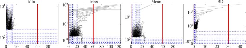
290               E. Quaeghebeur and M. B. Zaaijer: How to improve the state of the art in metocean measurement datasets

 4. We ran automated checks for outlier candidates. There                                  we see a quite large number of atypically high tem-
    can be both “classical” outliers, i.e., values outside                                 peratures and some impossibly fast 10 min temperature
    the range typical for that series, and “dynamic” ones,                                 changes, a couple of them of more than 30 ◦ C.
    i.e., subsequent value pairs whose difference (“rate of                                Outlier plots for all data series are available in the Sup-
    change”) lies outside the difference typical for that se-                              plement for this paper. The code producing them is pub-
    ries’s time variation. Both types of outliers can, but do                              licly available (Quaeghebeur, 2020).
    not necessarily, correspond to faulty data.
      In further manual analysis of outlier candidates, causes                           Our analysis was generic in the sense that we did not make
      may be identified, providing feedback on the data col-                          use of quantity-specific domain knowledge (e.g., empirical
      lection and processing procedures. For example, in both                         relationships between mean and maximum) or measurement-
      the MMIJ and FINO1 datasets, we encountered sudden                              setup-specific knowledge (e.g., met mast influence on wind
      drops to the value zero for some series at regular time                         speed). In the context of wind resource assessment, Brower
      instances; this quite likely corresponds to foreseeable or                      (2012) gives a description of a data validation procedure that
      detectable sensor resets of some kind.                                          does take into account such specifics. Meek and Hatfield
      There are many methods for outlier detection (Aggar-                            (1994) proposed signal-specific rules for checking meteo-
      wal, 2017). But, in this paper, we just wish to point out                       rological measurements for range violations, rate-of-change
      that there is a clear need for some form of outlier detec-                      outliers, and no-observed-change occurrences.
      tion to be used in the creation of metocean 10 min statis-                         For all of the issues presented in this section, the dataset
      tics datasets. Namely, the datasets we analyzed would                           producer is better placed to interpret them, given that they
      benefit enormously from even a basic analysis; we sus-                          have information about the data acquisition and processing
      pect this generalizes to other such datasets produced in                        procedures that the user lacks. Therefore it is the dataset pro-
      the wind energy field. To make this need apparent, we                           ducer who would ideally identify such issues and fix them,
      present a set of plots in Figs. 3–6 that illustrates that in-                   if possible, or otherwise at least mask or flag them. Given,
      deed there are still outliers present in the datasets. We                       as illustrated, the relative simplicity of the required analy-
      devised this type of plot as an alternative to lag-1 plots                      ses, relatively little effort may be required for a substantial
      (which plot xk+1 versus xk ), so that rate-of-change mag-                       increase in dataset quality.
      nitudes can be read off directly.
      These plots, of which examples are given in Figs. 3–6,                          2.2.2   Documentation
      should be read as follows. The horizontal x axis shows                          As mentioned in Sect. 2.1, for each of the three datasets we
      measurement value; the vertical y axis shows the ab-                            investigated, documentation on the measurement setup, in-
      solute value of the mean of the differences with the                            struments, and quantities measured is available. Usually, this
      preceding and next measurement values. Each dot cor-                            takes the form of a website, data manual, overview table, or
      responds to a measurement. Lines connect successive                             a combination thereof. However, for purposes of interpreta-
      measurements. Only those measurements are shown                                 tion and use of these datasets, some essential or potentially
      with an x percentile outside [0.1, 99.9] or a y percentile                      useful information is often missing.
      above 99, so the brunt of the measurements are not                                 We consider the information we listed in the overview Ta-
      shown. (These bounds are somewhat arbitrary, but rea-                           bles 1, A1, and A2 to be essential: instrument location, quan-
      sonable for the size of the datasets.) The y axis is linear                     tity measured, its unit, information about accuracy (e.g., by
      until the 99th percentile and logarithmic above. To give                        giving absolute and relative uncertainty)1 , range, and, given
      an idea about the distribution of all the measurement                           our focus on statistics data, sampling frequency. For categor-
      points, so also the ones that are not shown, we add (blue)                      ical data such as binary yes or no sensors (e.g., precipitation
      lines for specific fractiles: thick dashed for the median                       presence) or enumeration values (e.g., synoptic codes), range
      and thin dotted for { 216 , . . ., 18 , 14 , 34 , 78 , . . ., 1− 216 }. Thick   is of course replaced by a set of possible values and unit by
      full (red) lines are added as necessary to indicate range                       a description of how to interpret those possible values.
      bounds.                                                                            How do the three datasets fare in terms of documentation?
      In Fig. 3, there are some suspiciously high values, some                           1 We follow the Joint Committee for Guides in Metrology (2012)
      even beyond the nominal measurement range of the
                                                                                      in our usage of “(measurement) accuracy” and “(measurement) un-
      instrument. This is also the case for the “Min” and
                                                                                      certainty”. Namely, the former refers to a qualitative description of
      “Mean” statistics, even if the probably isolated respon-                        the “closeness of agreement between a measured quantity value and
      sible data points are not visible. In Fig. 4, there are sus-                    a true quantity value of a measurand” and the latter to a quantitative
      picious 0 % values and several values beyond 100 %. In                          measure, i.e., a “non-negative parameter characterizing the disper-
      Fig. 5, we see a cluster of data points at suspiciously                         sion of the quantity values being attributed to a measurand, based
      low values and some impossibly fast 10 min pressure                             on the information used”. These terms cover both systematic and
      changes, a number of them more than 100 hPa. In Fig. 6,                         random aspects.

Wind Energ. Sci., 5, 285–308, 2020                                                                             www.wind-energ-sci.net/5/285/2020/
E. Quaeghebeur and M. B. Zaaijer: How to improve the state of the art in metocean measurement datasets 291
Figure 3. Illustrative plots for visually identifying outliers (see text for an explanation): OWEZ 21 m NW ultrasonic anemometer horizontal
wind speed data (m s−1 ).
Figure 4. Illustrative plots for visually identifying outliers (see text for an explanation): MMIJ 21 m relative humidity data (%).
sponds to the raw data we have seen for OWEZ, we can
deduce the convention used. Based on whether the first
timestamp in a data file has “00” or “10” for its min-
utes value, we assume that OWEZ and MMIJ are first-
sample based and FINO1 is last-sample based.
Location For all three datasets, the documentation about lo-
cation was good to excellent: technical drawings of the
Figure 5. Illustrative plots for visually identifying outliers (see text mast with instrument locations or detailed data about
for an explanation): FINO1 21 m air pressure data (hPa). orientation and height. (Pictures or video footage would
of course further increase confidence in the accuracy of
the drawings.) A small comment we can make here is
that the location information in the series names used
sometimes does not directly correspond to the actual
situation. For example, in the MMIJ dataset a 46.5◦
angle offset of boom orientation relative to the (geo-
graphic) north needs to be accounted for and in the
FINO1 dataset some height labels differed from the doc-
umented heights.
Figure 6. Illustrative plots for visually identifying outliers (see text
for an explanation): FINO1 72 m ambient temperature data (◦ C). Quantities and units The description of the actual quanti-
ties measured and their units was in general also quite
good. There were two clear exceptions. (i) The precipi-
Timestamps All data values are accompanied by times- tation detector was completely omitted from the MMIJ
tamps spaced 10 min apart. However, for none of the documentation. (ii) Precipitation data from FINO1 at
three datasets is it mentioned whether this timestamp 23 m contained the concatenation of both presence (yes
refers to the time of the first, last, or even some other or no) and intensity data. Also, the interpretation of bi-
sample. Knowing this is necessary for the precise com- nary codes (e.g., does 0 correspond to yes or no?) was
bination of datasets. If we assume that the samples un- not explicitly given for any of the datasets, but had to be
derlying the dataset start at the full hour, which corre- deduced from the data.
www.wind-energ-sci.net/5/285/2020/ Wind Energ. Sci., 5, 285–308, 2020292 E. Quaeghebeur and M. B. Zaaijer: How to improve the state of the art in metocean measurement datasets
Ranges Ranges and sets of possible values were mostly left be other markers for faulty data. For FINO1, there
unmentioned in the documentation, except for those are two main faulty data placeholder values easily
available in instrument data sheets included in the identified from the datasets: −999.99 and −999.
OWEZ and MMIJ data manuals. Making the data sheets However, other values are also present, such as 0
of the instruments available in such a way turned out to and variants of the two main ones, such as 999,
be convenient, as tracking them down is, in our experi- −999.9, and −1000.
ence, not always possible. – How are the statistics calculated? This is never
Accuracy1 Accuracy information was available in the mentioned in the documentation. For most signals
FINO1 overview table and for those instruments for not much ambiguity can arise, as there is not much
which the data sheet was included in the OWEZ and choice, being limited to a possible bias correction
MMIJ data manuals. For the other signals, we had to approach for the standard deviation. However, for
rely on the information found in data sheets not avail- directional data, it is very much pertinent which
able in the datasets’ documentation or on their website. definition of mean and standard deviation have been
Entirely absent is a discussion of the impact on accu- used: arithmetic or directional mean, classical or
racy of all other aspects of the measurement setup (e.g., circular standard deviation (see, e.g., Fisher, 1995).
analog-to-digital conversion) and data processing (e.g., – Do the data processing steps to arrive at the statis-
the application of calibration factors). Such a discussion tics have any weaknesses, numerical or other? For
would allow researchers using the datasets to get a more example, in the FINO1 wind speed data, there ap-
complete picture of the accuracy of the values in the pear max values that, suspiciously, are a factor of
datasets. 10 or 100 times larger than the surrounding values.
Leaving such things unexplained severely reduces
Sampling frequency The sampling frequencies were avail- the trust in the dataset.
able in the documentation for MMIJ and FINO1, but not
for OWEZ. This information is essential for the estima- It is clear from the above list that while already a good
tion of the uncertainty of the mean and standard devia- amount of information is available, quite a number of very
tion statistics (see Sect. 2.2.5). useful pieces of information are missing. Many of these are
available to the dataset producers, so again the quality of the
Instruments and their settings We mentioned our use of
datasets, now in terms of documentation, can be substantially
data sheets a few times before. To find these when
improved with little effort relative to the whole of the mea-
they are not included in the documentation, the exact
surement campaign.
instrument models need to be available. This was the
Unmentioned as of yet is that essentially all the documen-
case for all three datasets. However, this may not be
tation for these datasets is provided in a way accessible to
enough: the measurement characteristics of some in-
humans, but not in a machine-readable way. Much of the in-
struments (e.g., barometers) depend on specific settings,
formation described in the documentation can however be
especially when they perform digital processing. These
encoded as metadata in a standardized and machine-readable
settings were never described. Furthermore, loggers are
way. Metadata are discussed further in Sect. 3.1.
an essential piece of the measurement chain and there-
fore need to be documented as well. For MMIJ and
FINO1 this is the case, but not for OWEZ. 2.2.3 Statistic selection
Data processing Next to its relevance for assessing the ac- As seen in the overview Sect. 2.1.1, 2.1.2, and 2.1.3, for all
curacy of the values in the dataset, a good view of the three datasets the statistics provided are essentially the same:
data processing pipeline is important for other aspects minimum, maximum, mean, and standard deviation. Only
as well. for FINO1 are not all statistics included for all quantities. In
this section, we are going to discuss these statistic selection
– When are data considered to be faulty and flagged choices, pointing out issues that arise from them.
in or omitted from the dataset accordingly? This is The uniformity of the statistics provided is convenient
entirely missing for OWEZ and FINO1, but some when reading out the data, as it reduces the user’s quantity-
information is given for MMIJ: if some values in specific code. However, when the signal’s values do not rep-
a 10 min interval are missing, the corresponding resent a (underlying) linear scale, providing the minimum,
statistics are marked as missing. How faulty data maximum, mean, and standard deviation does not make
values are encoded is documented for OWEZ (as much sense; it may actually cause misinterpretation. This is
the value −999 999), but not for MMIJ and FINO1. usually the case for categorical signals, such as the MMIJ
For MMIJ, the convention used (the string “NaN”) synoptic code signal. In such cases, other statistics must be
seems to be used quite consistently, although some chosen. For example, for binary quantities such as yes–no
precipitation monitor outlier values might actually precipitation data, giving the relative frequency of just one
Wind Energ. Sci., 5, 285–308, 2020 www.wind-energ-sci.net/5/285/2020/E. Quaeghebeur and M. B. Zaaijer: How to improve the state of the art in metocean measurement datasets 293
of the two values captures all the information present in the double for OWEZ. There is, however, more to be said about
typical set of four statistics. what exactly is encoded and which information can be re-
As said, in the FINO1 dataset statistics are sometimes flected in the encoding. We do that here.
omitted, but mostly for other reasons. For quantities that are Signal values have a natural set they belong to. Relative
considered to be “slow-varying” (such as atmospheric pres- humidity, for example, is a fraction, i.e., a value between
sure, ambient temperature, and relative humidity) only the zero and 1. Categorical signals take values in a predefined
mean has been recorded. However, next to the convenience enumerated set. If for such signals values are given outside
of uniform sets of statistics, having multiple statistics for of this set, this is a source of confusion: the user may wonder
a measurement interval is useful for data quality assessment. whether they can just round erroneous values to the near-
(Possible storage and transfer constraints are of course valid est enumerated one or treat them as faulty. For example, the
reasons for limiting the number of statistics.) For directional MMIJ precipitation detector’s precipitation presence signal
quantities such as wind direction, the minimum and maxi- contains values around the enumerated ones and its precipi-
mum were omitted because these are considered meaning- tation monitors’ precipitation presence signals contains val-
less by the dataset producer.2 The OWEZ and MMIJ datasets ues far outside the range of enumerated values. Another case
show, however, that it is possible to give meaningful defini- are continuous signals that are at one point expressed as cur-
tions of maximum and minimum for directional data. (See rent or voltage values: the end user will be less certain about
Appendix A2.1 for a concrete approach.) This can be valu- the correct translation procedure to the correct units than the
able information, as it makes it possible to deduce, for exam- data processor. For example, the FINO1 precipitation inten-
ple, the sector extent from which the wind has blown during sity signal is expressed as a current instead of an accumula-
a time interval. tion speed.
In the OWEZ and FINO1 datasets it sometimes occurs that
2.2.4 Quality flags certain statistics are marked as faulty or missing, while nev-
ertheless other statistics for the same signal at the same in-
Next to statistics, we saw in Sect. 2.1.3 that the FINO1 stance are available. From inspection of such data, it is clear
dataset also contains a categorical quality flag for each set that it can happen that the values of these other statistics seem
of statistics. Such information is not present in the other two reasonable or faulty. An explanation of why the data values
datasets. are partly missing would preserve trust in the non-missing
Including such a flag makes it possible to also provide values. This requires a description of the processes creat-
information about missingness, i.e., to indicate why one or ing such a situation (see Sect. 2.2.2), but could also include
more statistic values are missing at that time instant. Such instance-specific information in a flag value (see Sect. 2.2.4).
information is often encoded using a bit field, i.e., a binary The values stored in the dataset do not in general encode
mapping from quality issues and missingness mechanisms their accuracy. For the MMIJ and FINO1 datasets, values
to true (1) and false (0); this bit field can be recorded as used a fixed-point format, but the number of decimal digits
a positive integer. For example, consider the following tu- used is not directly related to the accuracy information avail-
ple of quality issues and missingness mechanisms: (“sus- able for the different quantities. This fact may be overlooked
pect value jumps”, “out-of-range values”, “unknown miss- by users, resulting in possible misinterpretations.
ingness mechanism”, “icing”, “instrument off-line”). Then To avoid misinterpretation, it is possible to add an esti-
the bit string “00000” (or integer 0) would denote a measure- mate for a value’s uncertainty, e.g., by rounding and speci-
ment interval without any (identified) issues and for example fying a corresponding number of significant digits. Accuracy
“010010” (or integer 18) would correspond to a measurement information was only available for signal values (i.e., high-
interval with both instrument icing and out-of-range values frequency samples), typically as absolute uncertainties εa
detected. and relative uncertainties εr . Below, we give expressions for
Of course other information next to missingness mecha- propagating this information to the statistics, as these do not
nisms can be included in the quality flag bit field, also for seem available in the literature, and we discuss further factors
non-missing values, as is done for FINO1. For example, this affecting the statistics’ uncertainty. The nontrivial deriva-
can be used to indicate possibly faulty data (see Sect. 2.2.1) tions of these expressions and a description of the underly-
that have not been removed (made missing). ing model for the measurement process can be found in Ap-
pendix A2.2. The most important assumption made in these
2.2.5 Value encoding and uncertainty propagation derivations is that εr2
1
n, where n is the number of
samples per averaging interval.
In the overview Sect. 2.1.1, 2.1.2, and 2.1.3, for all three
Sample uncertainties can be propagated to the statistics
datasets, the values themselves are encoded as fixed-point
of the n signal values xk per averaging interval, which is
values for MMIJ and FINO1 and as a binary floating point
10 min for the datasets discussed in this paper. For this, we
2 Personal communication on 27 June 2017 with Richard essentially assume independence and normality of the corre-
Fruehmann (see Acknowledgements). sponding uncertainties εxk . Also, the uncertainty in the statis-
www.wind-energ-sci.net/5/285/2020/ Wind Energ. Sci., 5, 285–308, 2020294 E. Quaeghebeur and M. B. Zaaijer: How to improve the state of the art in metocean measurement datasets
tics due to the finite nature of the samples can be quanti- wind speed, e.g., an average reduction of turbulence intensity
fied based on the fact that the sum appearing in the calcu- up to about 20 %.) But to be able to assess this impact, uncer-
lation of the mean and standard deviation can be seen as tainty and bias values must be available, making expressions
a simple form of quadrature. Let x̌ and x̂ be the
P minimum such as the above essential.
and maximum values in the sample; let x̄ = n1 nk=1 xk and Before closing this section, it is important to stress that the
sx2 = n1 nk=1 (xk − x̄)2 be the sample mean and sample vari- expressions for propagated uncertainties and biases above are
P
ance. We find the following expressions for the squared un- generic. Namely, their derivation does not depend on the spe-
certainties of the statistics: cific quantity considered or instrument used. Detailed knowl-
1 edge of the measuring instrument’s properties may allow
εx2 ≈ εa2 + εr2 x 2 + 2 δ 2 for x ∈ {x̌, x̂}, for better uncertainty estimates or additional uncertainty and
n bias terms. For example, for cup anemometers, it is known
2 1 2 1
that there is a positive bias of 0.5 %–8 % in the mean wind
εx̄ ≈ εa + εr x̄ + sx2 + 2 δ 2 ,
2 2
n n speed but that this bias can be greatly reduced using wind
1 1
direction variance estimates (Kristensen, 1999). Also, the
εs2x ≥ ε 2 + εr2 x̄ 2 + 3sx2 + 2 δ 2 .
n a n IEC 61400-12-1 standard prescribes how the wind speed un-
certainty should be calculated for calibrated cup anemome-
Here δ ≈ x̂−2 x̌ ; in case x̂ and x̌ are unavailable, δ ≈ z1−1/n sx ters (IEC, 2017, Appendix F), which may lead to high-quality
can be used instead, where z1−1/n is the standard normal estimates for εa and εr .
quantile for exceedance probability 1/n. The uncertainty due
to the finite sample size, the term n12 δ 2 , diminishes much
faster as a function of n than the uncertainty due to the mea- 3 Dataset formatting
surement noise, expressed by the other terms. In practice, this
second term is therefore negligible unless εa and εr are taken We split our discussion of dataset file formats into two parts.
to be zero because no information is available about them. First, in Sect. 3.1, we give an overview of the formats that are
Next to having associated uncertainties, the sample statis- currently used for the dissemination of the datasets studied
tics can also be biased estimators of the statistics for the un- and existing alternatives that we argue to be superior. Then,
derlying signal. It turns out that only the sample standard de- in Sect. 3.2, we take a closer look at the potential of these
viation sx is biased and that alternatives based on our practical experience with them.
q
sx0 = max sx2 − εa2 + εr2 x̄ 2 , 0 3.1 A comparison of dataset file formats
would be a better estimate from this perspective. We saw in Sect. 2.1, during our first look at the datasets we
To get a more concrete view of these uncertainties and studied, that these were disseminated as a compressed set of
bias, we provide average relative uncertainty and bias values Excel files for OWEZ, a compressed semicolon-separated-
for the MMIJ dataset in Table 3. (The code producing the re- value file for MMIJ, and a compressed set of tab-separated-
sults of this table is publicly available; Quaeghebeur, 2020.) value files for FINO1. In the Excel files, the values are
The variation in the uncertainties and bias is substantial, so stored as 8 B binary floating point numbers. In the delimiter-
this table of averages does not provide a complete picture, separated-value files the values are specified in a fixed-point
but enough to draw some conclusions. decimal text format, with five (MMIJ) and two (FINO1)
fractional digits. All of these are essentially table-based for-
– A fixed-point format does not have the flexibility to give mats, where columns correspond to series and rows corre-
the appropriate number of significant digits; usually ei- spond to values for a specific time instance. (This structure
ther too many or too few are given. satisfies the requirements of “tidy data” according to Wick-
ham (2014), apart from being split over multiple files.) Some
– While the uncertainty is usually rather small (up to a few
metadata are included in two or more header lines, such as
percent), in some cases it is substantial (around 10 % or
series identifiers and the unit.
more).
We created binary file format versions of the datasets; in
– The bias in the sample standard deviation can in general HDF5 format (The HDF Group, 2019a) for OWEZ and in
not be ignored. (For example, for ambient temperature, netCDF4 format (Unidata, 2018) for MMIJ and FINO1. Both
we see that the bias-corrected value is smaller than the formats are platform-independent. Files in netCDF4 format
uncertainty.) are actually HDF5 files, but adhering to the netCDF data
model (Rew et al., 2006). The use of a different data model
What the impact of uncertainty and bias is depends on the is reflected in the application programming interfaces (APIs)
application. (For example, turbulence intensity estimation is available for HDF5 and netCDF4. A number of HDF5’s tech-
clearly affected by the bias in the wind speed sample standard nical features are not supported by the netCDF data model,
s0
deviation. Concretely TI0 /TI = x̄x / sx̄x = sx0 /sx for horizontal which on the other hand provides additional semantic fea-
Wind Energ. Sci., 5, 285–308, 2020 www.wind-energ-sci.net/5/285/2020/E. Quaeghebeur and M. B. Zaaijer: How to improve the state of the art in metocean measurement datasets 295
Table 3. Average relative uncertainties and bias in percent for quantities from the MMIJ dataset for which some (likely incomplete) uncer-
tainty information is available. (See Table A1 for more information about the quantities. The values are given with two digits, but it is not
implied that both are significant.)
εx̌ εx̂ εx̄ εsx sx0 s0
Instrument Quantity 1− x
x̌ x̂ x̄ sx sx sx
Cup anemometer hor. wind sp. 4.3 2.7 0.067 1.0 81 19
Ultrasonic anemometer wind sp. X dir. 10 11 2.4 3.0 88 12
wind sp. Y dir. 11 12 2.4 3.0 89 11
wind sp. Z dir. 16 29 7.7 3.3 81 19
Wind vane wind direction 2.2 0.77 0.056 1.4 94 6.4
Barometer atm. pressure 0.017 0.0099 0.00021 7.2 5.2 95
Thermometer ambient temp. 2.3 2.3 0.067 35 4.4 96
Hygrometer rel. humidity 1.3 1.3 0.026 8.7 17 83
Precipitation monitor precip. intensity 17 17 0.45 3.4 98 2.0
Fromv,s cup anemometer hor. wind sp. 2.7 1.7 0.044 0.76 89 11
Fromv ultrasonic anemometer wind sp. magn. 3.9 3.0 3.0 3.4 97 3.5
hor. wind sp. 2.0 0.79 0.042 0.44 98 2.3
Fromv,s ultrasonic anemometer hor. wind sp. 1.2 0.58 0.045 0.31 99 1.2
Fromv,s wind vane wind direction 1.8 0.56 0.042 0.51 96 3.9
Fromv barometer and thermometer air density 0.016 0.0085 0.00018 2.0 72 28
s Correction for tower shadow by selective averaging of values at the same height.
v Virtual measurement, namely, derived from signals obtained with one or more actual instruments.
tures, most notably, shared dimensions and coordinate vari- to use them; they appear to be the most future-proof of the
ables. The netCDF4 format and its predecessors are popu- many binary formats in existence. We used Python modules
lar for the storage of Earth science datasets, including meto- to work with all these formats (McKinney et al., 2019; Co-
cean ones. These formats allow the data to be placed into lette, 2018; Unidata, 2019a).
multidimensional arrays, called “variables”, in a hierarchical Next let us consider the impact of a format being text-
file system-like group structure. Arbitrary key-value meta- based or binary-based. Text-based formats in principle give
data attributes can be attached to both groups and variables. a lot of freedom in choosing the format in which values are
The variables support various common data types, such as represented, but usually this is done in a single fixed-point
1, 2, 4, and 8 B integers; 2, 4, and 8 B binary IEEE float- format. To use the data, the values’ representations need to
ing point numbers (Cowlishaw, 2008); and character strings. be parsed into the standard binary number formats used by
Also, custom enumerations, variable-length arrays, and com- computers, namely floats and integers of various kinds. Bi-
pound types can be defined, e.g., a combination of four floats nary file formats use binary number formats directly, which
and an integer. Furthermore, variables can be compressed are faster to load into memory and more space-efficient.3
transparently, i.e., without the user having to manually per- Because of their standardized nature, they can include other
form decompression before use. binary-specific features, such as transparent compression and
Let us give a brief evaluation of support in software tools checksums (data integrity codes).
for the different file formats. Even if the delimiter-separated- Now let us look at the metadata. HDF5 and netCDF4 are
value files are not really standardized (however, see Lindner, considered self-describing formats, as they allow arbitrary
1993; Shafranovich, 2005), support for them is near univer- metadata to be included next to the data. These data are easy
sal. Software tools usually include options to deal with the to access, also programmatically. Table-based data files typi-
particulars of the actual encoding (delimiter, quoting, head- cally include one or two header lines of metadata (sometimes
ers, etc.), but this does require manual discovery of these
3 In text files, every decimal digit costs 8 bits (1 B) to store, so
specifics. These text-based formats can in principle be read
and modified in a text editor, but these are usually not de- a length-n number requires 8n bits. In binary formats, a more effi-
signed to deal with large files, so this is actually impracti- cient encoding is used (numbers as bit strings), requiring m bits. To
round-trip from decimal to binary and back, m = bnlog2 (10)+2c ≈
cal for all but the smallest datasets. The Excel “xls” format,
b3.3n+2c is sufficient (Matula, 1968). This picture does not change
even though proprietary, has broad reading support. Support
substantively if sign and magnitude are taken into account. In prac-
for HDF5 and netCDF4 formats in software tools is very ex- tice a 32-bit binary format is used for storing values, which uses
tensive (The HDF Group, 2019b; Unidata, 2019b). This, in 23 bits for representing the significand, sufficient for six decimal
addition to their feature set, is also a reason for us choosing significant digits; 1 bit is used for the sign and 8 for the exponent.
www.wind-energ-sci.net/5/285/2020/ Wind Energ. Sci., 5, 285–308, 2020296 E. Quaeghebeur and M. B. Zaaijer: How to improve the state of the art in metocean measurement datasets
more), but there is no universal convention about what can be “not a number” binary floating point value is the com-
found there. So making use of information included in this mon approach we followed. Using a Boolean mask sep-
way always requires user intervention. There are initiatives to arate from the dataset itself is an alternative that can also
create metadata inclusion standards for delimiter-separated- be used in case the data stored do not consist of floating
value formats, but these have not gained significant adoption point values.
and are aimed at either web-based material (Tennison et al.,
2015) or small datasets (Riede et al., 2010), or they are very 2. One must decide on and create a structure for the file, to
recent proposals (Walsh and Pollock, 2019). organize the data and make them conveniently accessi-
Section 2.2.2 mentioned that the documentation available ble. We used a hierarchical structure for this, grouping
for the datasets we investigated is not machine-readable. It first by device (class) and then by quantity. For instru-
can be made so by providing it as metadata. Such metadata ment locations, we tried two approaches:
can be used to facilitate analyses and uses of the data. For ex-
ample, if a tool has access to the range and units associated – adding the locations as groups in the hierarchy, be-
with series of values, air pressure, and temperature, say, then low the “quantity” groups (done for OWEZ);
it can automatically determine those for derived series, such – collecting the data for all locations in a multidimen-
as air density. Examples of metadata standards for datasets sional array with additional axes next to the time
are the “CF Conventions” (Eaton et al., 2017), ISO 19115-1 axis, e.g., for height and boom direction (done for
(ISO/TC 211, 2014), and the recently developed “Metadata MMIJ and FINO1).
for wind energy Research and Development” (Sempreviva
et al., 2017; Vasiljevic and Gancarski, 2019). It is encour- For the different statistics (minimum, maximum, mean,
aged in the Earth science community to not just add arbitrary and standard deviation), we tried three approaches:
metadata, but also include at least standard attributes from
the “CF Conventions” (Eaton et al., 2017) and follow the – adding the statistics series as separate variables in
“Attribute Convention for Data Discovery” (Earth Science the hierarchy (done for all three);
Information Partners, 2015). These facilitate reuse and dis- – keeping the statistics together in a compound data
covery and also make it possible, for example, for software structure, essentially a tuple of values, where each
to enhance the presentation of the dataset elements (see, e.g., value is accessed by (statistic) name; such com-
Hoyer et al., 2018). They also allow for adding further useful pound values then formed the elements of the mul-
metadata, such as provenance information, e.g., in the form tidimensional arrays (done for MMIJ and FINO1);
of an ISO Lineage (ISO/TC 211, 2019). These conventions
are aimed at netCDF files, but can to a large degree be applied – adding the statistics as an extra axis to the multidi-
to HDF5 files as well. Of course the metadata to be included mensional array (done as well for MMIJ).
as recommended by these conventions can also be specified
for table-based formats, but not in the same self-describing 3. One must collect and compose the metadata for the
way. dataset, the devices, and the quantities. Then one must
add these as attributes in the file. The latter is almost
trivial to do once the former time-consuming task is
3.2 Practical experiences with binary formats completed.
We already mentioned in Sect. 2.2.1 that we created binary 4. One must choose an encoding and the storage parame-
HDF5 and netCDF4 file versions of the datasets we studied. ters for the data and write them out to the file. We chose
In this section, we first, in Sect. 3.2.1, report on the process to store the values as 4 B binary floating point numbers,
and its results. Then, in Sect. 3.2.2, we discuss the limitations compress them using the standard “Deflate” algorithm,
of these formats, including limitations of software support. and add error detection using “Fletcher-32” checksums.
Furthermore, we used the information available about
3.2.1 The transformation process the accuracy of the values to round to the least signif-
icant binary digit. This is a lossy transformation that,
Transforming the supplied data files was done by writing however, does not lose significant information, but fur-
a specific script for each case. The general setup is similar ther improves compression.
for each script.
Let us finish this section with some remarks.
1. One needs to import the supplied datasets into in-
memory data structures that can be manipulated by the – During the transformation process, we could load the
scripting language. An important part of this step is the datasets studied entirely into memory. This is conve-
identification of missing data or data marked as faulty nient, but not necessary, as the process of reading the
and encoding them appropriately. Storing them as the supplied datasets can be done in a piece-wise fashion.
Wind Energ. Sci., 5, 285–308, 2020 www.wind-energ-sci.net/5/285/2020/E. Quaeghebeur and M. B. Zaaijer: How to improve the state of the art in metocean measurement datasets 297
– The size of the files resulting from the transformation x is equal to αk + β within required precision. HDF5
we made was one-eighth of the supplied files’ size or has a built-in filter to do this, but it does not preserve
smaller and one-half their compressed size or smaller. special floating point values like NaNs used for rep-
(More precisely, the sizes of the uncompressed (com- resenting missing values. The CF Conventions (Eaton
pressed) supplied files versus the sizes of our HDF5 et al., 2017) often used in netCDF files also describe
or netCDF4 versions are as follows: OWEZ: 1 GB a metadata-based approach, but not all software auto-
(400 MB) vs. 65 MB; MMIJ: 500 MB (120 MB) vs. matically applies the inverse transformation, so it is not
55 MB; FINO1: 800 MB (120 MB) vs. 50 MB.) transparent to the user.
– Tools exist to facilitate the transformation process, most Dimensions When creating variables, the netCDF4 format
notably the online service Rosetta (Unidata, 2013), requires using defined “dimensions” (e.g., time and
which generates netCDF files satisfying the CF Con- height). These can be shared between variables and as-
ventions. sociated with “coordinate variables” (e.g., arrays with
concrete time values and instrument heights). There is
– Templates to facilitate the creation of netCDF files satis- also a similar concept of “dimension scale” in HDF5,
fying the CF Conventions and the Attribute Conventions but it is not as convenient.
for Data Discovery are available (NOAA National Cen-
ters for Environmental Information, 2015). These do not Unicode In principle both HDF5 and netCDF4 support Uni-
make use of hierarchical grouping, but can to a large de- code text for group, variable, and attribute names and
gree be used within each group. for attribute values. Software support for Unicode text
in attribute values is not universal, however; notably,
3.2.2 Limitations of binary formats tested MATLAB does not support this yet for netCDF4.
When creating the transformed dataset files, we tested many String values Both HDF5 and netCDF4 support variable-
of the features available in the HDF5 and netCDF4 formats. length strings as variable values. This can for exam-
Not all of these features turned out to be as useful as initially ple be useful for coordinate variables, such as when
expected or have sufficient software support. We here dis- instrument position is designated by “left” and “right”.
cuss features for which we encountered issues, to help others However, again MATLAB does not support this yet for
make an informed choice when considering their use. netCDF4.
Compound data structures Compound data structures are 4 Recommendations
essentially tuples of values, where each component
value is accessed by its name. These allow for a tight Based on our analysis of the three datasets and on our work
grouping of related data, for example to group all the transforming them into binary file formats, we have the fol-
statistics for a given signal for a given measuring inter- lowing recommendations for the three main stakeholders.
val, to attach a quality flag, or to group the components (We also briefly indicate their role in the shared responsi-
of a vector (e.g., the wind velocity). However, metadata bility for creating high-quality, well documented, and usable
cannot be attached to the structure’s components, and to datasets.)
read any one component the whole structure is loaded
in memory, multiplying the memory requirements. Fur- Project owner (Through the “scope of work” part of the
thermore, support for creating these structures for use contract with the dataset producer, this party can specify
in netCDF4 files using Python was buggy and support requirements for the dataset format, quality, and docu-
for reading compound value data is currently far from mentation, so that it meets the needs of the considered
universal; for example, it is not included in MATLAB’s dataset users.)
netCDF interface. Also, documentation of their use is – Require the dataset producer to provide the datasets
currently limited. in a standardized binary format.
2 B floating point numbers HDF5 allows the storage of 2 B – Agree with the dataset producers about a concrete
(16-bit) floating point numbers, which is more space- level of quality control.
efficient if the precision is sufficient. The support in the – Require the datasets to be accompanied by (explic-
core HDF5 library turned out to be buggy and support itly specified) extensive metadata and documenta-
was non-existent, e.g., in MATLAB. tion, including accuracy and quality information.
Scale-offset filters Another approach for efficiently storing Dataset producers (Next to being responsible for produc-
floating point values x is to transform them to integer ing the dataset, this party can inform the project owner
values k of shorter bit length, namely choosing series- about the possibilities for dataset creation and the
specific scale and offset parameters α and β such that dataset users about efficient dataset use.)
www.wind-energ-sci.net/5/285/2020/ Wind Energ. Sci., 5, 285–308, 2020You can also read