Land-Water Interoperable Models - Project Summary Prepared for Our Land and Water - Our Land & Water
←
→
Page content transcription
If your browser does not render page correctly, please read the page content below
Land-Water Interoperable Models
            Project Summary

       Prepared for Our Land and Water

                 June 2020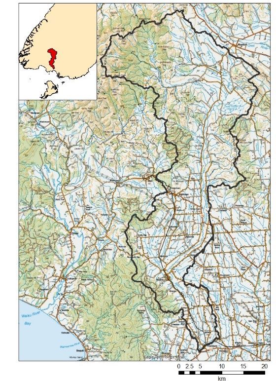
Prepared by:
Sandy Elliott1, Tom Evans1, Rogerio Cichota2, Utkur Djanibekov3
Alex Herzig3, Bethanna Jackson4, Daniel Lagrava Sandoval1
Stephen McDonald5, Juan Monge6, Annette Semadeni-Davies1
Mike Taves7, Christophe Thiange8, Ronaldo Vibart5, Steve Wakelin9, Sharleen Yalden1, Jing Yang1,
Harry Yoswara5

1
  NIWA
2
  Plant and Food Research
3
  Manaaki Whenua – Landcare Research New Zealand
4
  Victoria University of Wellington
5
  AgResearch
6
  Market Economics
8
  DairyNZ
7
  GNS Science
9
  Scion

For any information regarding this report please contact:
Sandy Elliott
Principal Scientist
Catchment Processes
+64-7-859 1839
National Institute of Water & Atmospheric Research Ltd
PO Box 11115
Hamilton 3251
Phone +64 7 856 7026

NIWA CLIENT REPORT No:      2020182HN
Report date:                June 2020
NIWA Project:               AGR19202

    Quality Assurance Statement

                                 Reviewed by:                                    Neale Hudson

                                 Formatting checked by:                          Rachel Wright

                                 Approved for release by:                        Scott Larned

© All rights reserved. This publication may not be reproduced or copied in any form without the permission of
the copyright owner(s). Such permission is only to be given in accordance with the terms of the client’s contract
with NIWA. This copyright extends to all forms of copying and any storage of material in any kind of
information retrieval system.

Whilst NIWA has used all reasonable endeavours to ensure that the information contained in this document is
accurate, NIWA does not give any express or implied warranty as to the completeness of the information
contained herein, or that it will be suitable for any purpose(s) other than those specifically contemplated
during the Project or agreed by NIWA and the Client.
Contents
Executive summary ............................................................................................................. 6

1       Introduction ............................................................................................................ 10

2       Overview of the modelling approach ........................................................................ 11
        2.1      Model integration software .................................................................................... 11
        2.2      Model components................................................................................................. 11
        2.3      Standards and linkage ............................................................................................. 12
        2.4      Introduction to the Aparima case study ................................................................. 14

3       Model standards and approaches adopted ............................................................... 16
        3.1      BMI as the standard for linking............................................................................... 16
        3.2      Naming conventions ............................................................................................... 17
        3.3      File formats ............................................................................................................. 20
        3.4      File-based coupling approach ................................................................................. 22

4       Model components .................................................................................................. 24
        4.1      Web service for retrieval of pre-computed stream flows ...................................... 24
        4.2      Nitrogen loss lookup ............................................................................................... 25
        4.3      Overseer nitrogen loss ............................................................................................ 27
        4.4      Steady state nitrogen routing in streams ............................................................... 29
        4.5      Steady state groundwater routing.......................................................................... 30
        4.6      Soil moisture accounting/rainfall-runoff model (subcomponent of LUCI) ............. 32
        4.7      Dynamic groundwater flow model ......................................................................... 33
        4.8      Dynamic stream flow routing ................................................................................. 35
        4.9      APSIM dynamic nitrogen source simulation ........................................................... 36
        4.10 Dynamic groundwater nitrogen routing ................................................................. 39
        4.11 Dynamic stream contaminant routing .................................................................... 41
        4.12 Economics and optimisation ................................................................................... 43

5       Model assemblies .................................................................................................... 46
        5.1      Linkage diagrams .................................................................................................... 46
        5.2      Linkage of components ........................................................................................... 48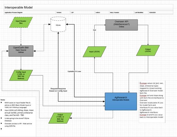
6 Incorporation of models into the Delta Shell environment ........................................ 49
6.1 Setting up and running models in the interactive environment ............................ 49
6.2 Visualisation of results ............................................................................................ 49
7 Model sharing and documentation ........................................................................... 53
8 Intellectual property, governance and co-ordination................................................. 54
8.1 Approaches used in the project .............................................................................. 54
8.2 Some future governance and management needs ................................................ 55
9 Recommended future technical approach to interoperability.................................... 56
10 Summary of key results and findings ........................................................................ 58
11 Acknowledgements ................................................................................................. 60
12 References............................................................................................................... 61
Tables
Table 4-1: BMI interfacing functions for the flow routing code. 35
Table 4-2: Summary of contaminant routing model operation via Initialize()
and Update() functions. 42
Figures
Figure 2-1: Schematic of components coupled in Delta Shell. 12
Figure 2-2: Aparima case study location. 14
Figure 2-3: Schematic summarising the ecotope generation process. 15
Figure 3-1: A representative model result, presented in SQLite Browser. 21
Figure 3-2: Example hydrograph from the LUCI model. 22
Figure 4-1: Sequence diagram of interaction between a master controller and
target point model component. 26
Figure 4-2: Schematic of the as-designed data flow for the nitrogen leaching loss
model. 28
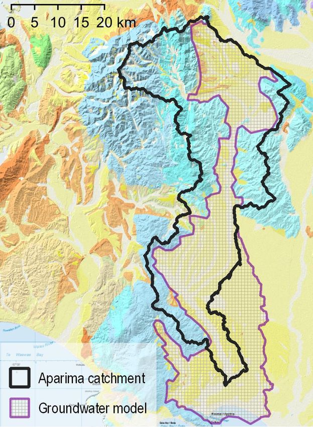
Figure 4-3: Map showing boundaries of Aparima catchment, groundwater model
and QMAP geology (Turnbull and Allibone 2003). 32
Figure 4-4: Schematic showing how data were exchanged between APSIM and the
Interoperable Model framework using several bespoke tools. 37
Figure 4-5: Schematic showing how data were exchanged between APSIM and the
Interoperable Model framework using coordinated by the APSIMHandler. 38
Figure 4-6: Example instruction file used by the APSIM Handler to run a scenario
involving several cropping rotations to determine fertiliser management
options. 39
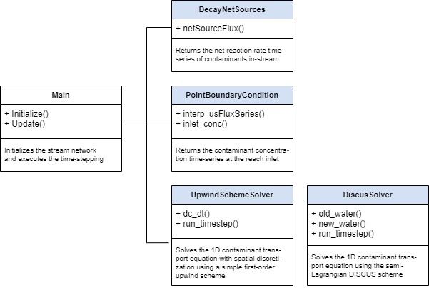
Figure 4-7: Class structure of dynamic stream contaminant routing model. 42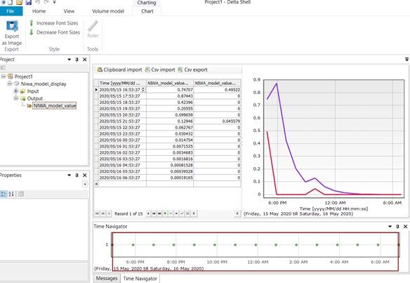
Figure 5-1: Example of a prototype 'wiring diagram' depicting model components
and their interactions for the static nitrogen model. 47
Figure 6-1: Example of prototype of data visualisation of flow time-series retrieved
through a web service and displayed within Delta Shell. 50
Figure 6-2: Example of map display of flow results for dynamic hydrologic model
for the Aparima catchment. 51
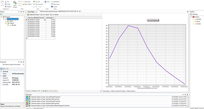
Figure 6-3: Example of display of flow time series from the dynamic hydrologic
model for the Aparima catchment. 52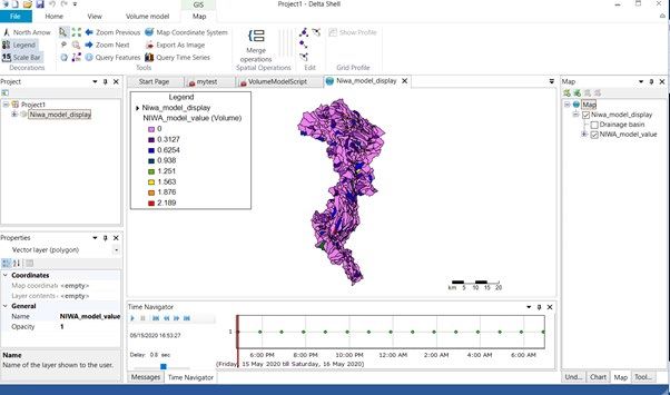
Executive summary
Project purpose and scope
This report is the final project report for Stage 2 of the “Interoperable Modelling Systems for
Integrated Land and Water Management” programme in the Our Land and Water National Science
Challenge (OLW). The programme addresses Theme 2 of the Challenge by providing modelling tools
to support “Innovative and resilient land and water use”, and Theme 3 by building collaborative
capacity within the modelling and model-user communities.

The programme aimed to develop an interoperable modelling system that is suitable for national use
in integrated spatial assessment of environmental, production and economic implications of land use
and land use change. The uses of the system will include assessment and accounting of productivity
potential and water quality contaminant dynamics at farm and catchment scales.

Interoperability refers to an approach to modelling whereby individual model components are
coupled in a flexible way including exchanging data between components, allowing for re-use and
substitution of model components within an overarching framework. It is proposed that the
availability of better, more trusted, and targeted modelling tools within an interoperable modelling
framework will result in more effective use of integrated modelling for improved production and
environmental management.

A staged approach has been developed to achieve these aims. Stage 1 of the programme established
a proposal for work to be undertaken in Stages 2 and 3 of the programme, and was documented
previously (Elliott et al. 2017). Stage 2, which is the subject of this report, focussed on implementing
and demonstrating the initial set of models and data within the framework. Stage 3 (anticipated for
tranche 2 of OLW) proposes to enrich the range of models in the framework and demonstrate and
evaluate the use of the framework in multiple contexts, including linking to social and cultural
attributes.

Work for this stage was conducted by a Technical Group from eight science organisations (NIWA,
AgResearch, DairyNZ, GNS Science, Manaaki Whenua/Landcare Research, SCION, and Victoria
University of Wellington) which incorporates specialists from a range of science providers, covering
the required areas of technical expertise- including catchment hydrology, production systems, water
quality, agro-economics and computer science.

Key aspects of the modelling
Interoperable models require software to co-ordinate running of the various model components and
managing data exchange. In this project, a system called Delta Shell was selected, following
assessment of such frameworks in Stage 1. Delta Shell 1 was developed by Deltares for model
coupling, user interaction, and visualising input and output datasets, and some of their core hydraulic
and water quality models have been set up in Delta Shell. Delta Shell operates in the Microsoft
Windows environment and is based on the Microsoft .Net C# language. It runs on a desktop
computer. The user interface includes mapping and time-series display components 'out of the box'.

Following workshops at the start of the project, twelve model components of key interest to OLW
were selected for implementation in Delta Shell. The components were organised into a set of static
models (not time-stepping) and a set of dynamic models, covering key aspects of catchment
hydrology and water quality. An economic, production, and optimisation component was also set up.

1   https://oss.deltares.nl/web/delta-shell

6                                                                       Land-Water Interoperable Models
These components demonstrate some key aspects that an interoperable system of models for land-
water needs to cater for. Each component was set up using a standard model interface, the Basic
Model Interface (BMI), and established for the case study site (Aparima catchment in Southland). The
static components that were implemented are:
Lookup table for nitrogen loss.
Nitrogen transport through groundwater – MODFLOW.
Nitrogen transport in streams – CLUES stream transport component.
Production, economics and optimisation (LUMASS).
Overseer nitrogen loss (partially completed).
The dynamic components that were implemented are:
Web service to query pre-computed time series from the TopNet hydrologic model.
Soil moisture accounting/rainfall-runoff model – from LUCI.
Dynamic groundwater flow – MODFLOW.
Dynamic stream flow routing (from TopNet).
Dynamic nitrogen loss – APSIM soil-plant model.
Dynamic groundwater nitrogen transport – MODFLOW.
Stream nitrogen transport.
Delta Shell contains a set of interface specifications (objects and methods) that can be used for
model components. Adopting those specifications would mean committing to a somewhat complex
interface that is specific to Delta Shell, .NET, and the desktop computing environment. Instead of
using Delta Shell's own specification, we decided to use an interface standard called BMI (the Basic
Model Interface), which is open source and used by multiple frameworks. Deltares' own models are
migrating more to using BMI, and Delta Shell has ways to run components that are set up with BMI.
Hence BMI was considered by the technical group to be a preferable interface.
Two key sets of linked components ('assemblies') were set up to trial and demonstrate model
coupling. They were a set of static models for nitrogen generation and transport, and a set of models
for dynamic runoff generation and transport. In the dynamic model, the model components could
exchange information at each time-step.
These components were linked using the DIMR (Deltares Integrated Model Runner) programme
within Delta Shell. The programme specifies the components used in an assembly and their order of
running, while allowing for dynamic models to exchange data each time-step (hence allowing
feedback between components). An interoperable modelling system requires a mechanism to
exchange data between model components. The BMI standard provides mechanisms for passing data
through common memory, but we found that the DIMR implementation of BMI, and the BMI
specification in general, had restrictions which were too limiting. To overcome this limitation, we
adopted a file-based data exchange approach, using the set of standard files.
A set of standard file formats and naming conventions was adopted, to organise and facilitate data
interchange. The file formats are well-recognised open standards, and many software programmes
have methods to read in and output such data. A set of naming conventions based on Community
Land-Water Interoperable Models 7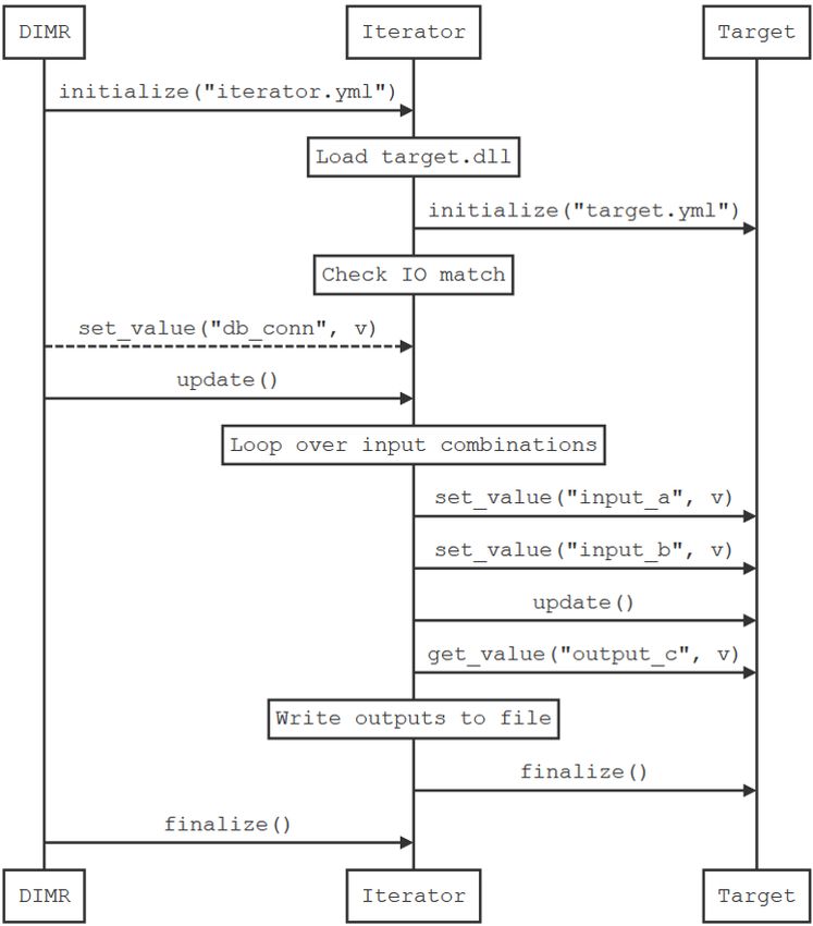
Surface Dynamics Modeling System (CSDMS) standard names was also adopted, although we
customised the names to better represent the types of model quantities that are needed for land-
water modelling.

We adopted an 'ecotope' approach to spatial representation, which involved conducting simulations
for each spatial unit defined by the intersection of property boundary, land use, soil class, climate
zone, irrigation (whether present) and slope class, which can be mapped onto a common grid basis.
In hydrological modelling such areas are more commonly known as HRUs (Hydrological Response
Units) – we have used the name ecotope to reflect an intention for application to both land and
water modelling. The results from each ecotope then provided inputs for other models, such as
inputs to each stream segment, after results were summarised at the subcatchment basis (based on
the grid of ecotope locations in conjunction with subcatchment boundaries). This approach allows for
future extension, for example, introducing other spatially-varying driving factors, allowing farm
management variables to vary by property, or for farm-level predictions to take account of farm
system behaviour. However, some limitations remain, such as the inability to represent the detailed
placement of edge-of-field mitigation measures or individual paddock management.
We used a GitHub document repository to share model components, assemblies, data and related
software. This system is publicly-available and widely used for software development projects. We
did not use version management or revision facilities of Git in the current project, mainly because
individuals or small groups were responsible for developing and maintaining their own components.
However, we envisage more sophisticated use of Git in the future.
Model components and assemblies were tested in the Aparima catchment (1280 km2) upstream of
Thornbury (Figure 2-2), which has multiple land uses but is dominated by pasture. The Aparima
model components and model assemblies were not calibrated or applied to scenarios – such work
was outside the scope of the current project. The main emphasis was to demonstrate how the model
components and assemblies could be set up and run in a real catchment.

Key results and recommendations
The project team succeeded in implementing a set of coupled models within an interoperable
modelling framework, with application in a trial catchment. This meets the key technical
requirements for this Stage of the programme.

Eleven model components covering water quantity, quality, production and economics were set up
within a framework (Delta Shell) using established standards for model interfaces (BMI), variable
naming (from CSDMS) and various standard file formats. We also attempted to implement Overseer,
but could not fully achieve this, partly due to reliance on an organisation external to the project
team.

Two sets of model components were successfully combined into assemblies to address a) steady
state contaminant transport and b) dynamic coupled flow calculation. The catchment models
resolved to the level of property, soil, climate class, and topographic class variation, using a common
spatial framework of 'ecotopes'.

In addition, models for production, economics, and environmental losses were set up using the BMI
in conjunction with the LUMASS optimisation engine.

As a separate exercise, we demonstrated how pre-computed flow time-series that are stored in an
external server could be imported and displayed within Delta Shell using Sensor Observation Service
(SOS) standards and a Delta Shell plug-in accessing data provided through that standard.

8                                                                       Land-Water Interoperable Models
We decided that it was preferable to use BMI instead of Delta Shell's native interface, to allow
greater flexibility and component re-use. However, we found that some key aspects of BMI were not
fully implemented in the Deltares model runner/coupler DIMR. Some simplifications and work-
arounds in our coupling approach were therefore required.

We found that file-based data exchange overcame limitations of BMI's interface for memory-based
data exchange (for example, BMI does not allow for tabular data to be exchanged or implemented).
The wide and multi-language availability of libraries for reading and manipulating the chosen
standard file formats assisted with importing and exporting data from model components. File-based
exchange could potentially become a problem with closely-coupled models that need to exchange
data frequently; in those circumstances, memory-based exchange may need to be implemented.

The models were set up for a trial catchment, the Aparima, and assemblies were run successfully
within the DeltaShell environment.

Model output was able to be displayed within the Delta Shell environment using the visualisation
libraries and user interface native to Delta Shell, although some additional code was required to
import model outputs into the DeltaShell environment.

All the model components, apart from Overseer, have been provided as free and open-source
components available on a data repository.

Despite these successes, the project team recommends that an alternative coupling approach based
on running model components be trialled. Such a system has several advantages over the Windows
desktop approach of Delta Shell. The requirements for framework software, and developer expertise
(to set up and orchestrate model assemblies) remain.

We used an ad-hoc 'wiring diagram' approach to defining linkages, data exchanges and timing. It
would be desirable to develop more formalised methods in the future, although standard URL
diagrams are not particularly suited to this purpose.

The project technical team developed good structured working relationships with ongoing
collaborative and collegial interactions. It was also desirable to introduce a project manager to
facilitate administrative task and performance monitoring. The governance group was increasingly
less involved with the project over time, an aspect that should be improved in future work. We also
identified that is important to use a software developer or group of developers with good computer
science knowledge, alongside model specialists.

This project has met the key technical requirements of this stage of the programme. It is anticipated
that a workshop will be held in the future to present key findings and recommendations, and to
consider a pathway forward, including future funding, governance, and IP considerations.

Land-Water Interoperable Models                                                                         9
1 Introduction
This report is the final project report for Stage 2 of the “Interoperable Modelling Systems for
Integrated Land and Water Management” programme in the Our Land and Water National Science
Challenge (OLW). The programme addresses Theme 2 of the Challenge by providing modelling tools
to support “Innovative and resilient land and water use”, and Theme 3 by building collaborative
capacity within the modelling and model-user communities.
The programme aimed to develop an interoperable modelling system that is suitable for national use
in integrated spatial assessment of environmental, production and economic implications of land use
and land use change. The uses of the system will include assessment and accounting of productivity
potential and contaminant dynamics at farm and catchment scales. The latter include nitrogen,
phosphorus, suspended sediment and microbial contaminants.
Interoperability refers to an approach to modelling whereby individual model components are
coupled in a flexible way that permits exchange of data between components, allowing for re-use
and substitution of model components within an overarching framework. It is proposed that the
availability of better, more trusted, and targeted modelling tools within an interoperable modelling
framework will result in more effective use of integrated modelling for improved production and
environmental management.
A staged approach has been followed to achieve these aims. Stage 1 of the programme established a
proposal for work to be undertaken in Stages 2 and 3 of the programme, and was documented in a
report (Elliott et al. 2017). Stage 2, which is the subject of this report, focussed on implementing and
demonstrating the initial set of models and data within the framework. Stage 3 (anticipated for
tranche 2 of OLW) proposes to enrich the range of models in the framework and demonstrate and
evaluate the use of the framework in multiple contexts, including linking to social and cultural
attributes.
Work for this stage was undertaken by a Technical Group comprising researchers from eight science
organisations (NIWA, AgResearch, DairyNZ, GNS Science, Manaaki Whenua/Landcare Research,
SCION, Victoria University of Wellington). This collaborative approach made specialists from a range
of science providers available to the project, covering the required areas of technical expertise. These
included catchment hydrology, production systems, water quality, agro-economics and computer
science.
This report:
Provides an overview of the approach taken to model interoperability.
Describes the standards and conventions used in this project.
Presents information on each of the model components, including how they were set
up and application in the case study.
Describes how the model components were linked and applied in the integration
software, including visualisation.
Identifies key intellectual property management, governance, and stewardship needs.
Recommends future approaches to interoperability.
10 Land-Water Interoperable Models2 Overview of the modelling approach
This section provides an overview of the model integration steps and approaches taken in this study,
which are described in more detail later in the report.
2.1 Model integration software
Interoperable models require software to co-ordinate running of the various model components and
manage data exchange. In the Stage 1 report (Elliott et al. 2017), a model framework called CSIP was
recommended, but following discussions with stakeholders, the second alternative, Delta Shell was
selected for use in Stage 2.
Delta Shell 2 (Donchyts et al. 2014; Deltares 2020) is a system developed by Deltares for model
coupling, user interaction, and visualising input and output datasets. Some of the core hydraulic and
water quality models created by Deltares have been set up in Delta Shell. It is free and largely open-
source, which was an important criterion for adoption in the OLW project. Deltares also provides free
hydrodynamic and water quality software, which was a further reason for adoption of Delta Shell in
the OLW project. Delta Shell is based on Microsoft Windows and utilises the Microsoft .NET C#
language. It runs on a desktop computer. The user interface includes mapping and time-series display
components 'out of the box'.
2.2 Model components
Following workshops at the start of the project, several model components of key interest to OLW
were selected for implementation in Delta Shell. These components were organised into a set of
static models (not time-stepping) and a set of dynamic models, covering key aspects of catchment
hydrology and water quality. An economic, production, and optimisation component was also
envisaged. These components demonstrate some key aspects that an interoperable system of
models for land-water management needed to cater for, but without addressing every need. Each
component was set up using a standard model interface, the Basic Model Interface 3, and established
for the case study site (the Aparima River catchment in Southland). The components, which are
detailed later in the report, are:
Static model components
Lookup table nitrogen loss.
Nitrogen transport through groundwater – MODFLOW.
Nitrogen transport in streams – CLUES stream transport component.
Production, economics and optimisation (LUMASS).
Overseer nitrogen loss (partially completed).
Dynamic model components
Web service to query pre-computed time series from the TopNet hydrologic model.
Soil moisture accounting/rainfall-runoff model – from LUCI.
Dynamic groundwater flow – MODFLOW.
2 https://oss.deltares.nl/web/delta-shell
3 https://bmi-spec.readthedocs.io/en/latest/ - a set of functions for querying, modifying, and running models
Land-Water Interoperable Models 11 Dynamic stream flow routing (from TopNet).
Dynamic nitrogen loss – APSIM soil-plant model.
Dynamic groundwater nitrogen transport – MODFLOW.
Stream nitrogen transport.
2.3 Standards and linkage
2.3.1 Component interface standards
Delta Shell contains a set of interface specifications (objects and methods) that can be used for
model components. Adopting those specifications would mean committing to a somewhat complex
interface that is specific to Delta Shell, .NET, and the desktop computing environment.
Instead of using Delta Shell's own specification, we decided to use an interface standard called BMI
(the Basic Model Interface), which is open and used by multiple frameworks. Deltares' own models
are migrating more to using BMI, and Delta Shell has ways to run components that are set up with
BMI. Hence BMI was considered by the technical group to be a preferable interface.
2.3.2 Model assemblies
Two key sets of linked components ('assemblies') were set up to trial and demonstrate model
coupling, as shown schematically in Figure 2-1.
These model components were coupled using the programme DIMR (Deltares Integrated Model
Runner) within Delta Shell. The programme specifies the components used in an assembly and their
order of running, including allowing for dynamic models to exchange data each time-step (hence
allowing feedback between components). While BMI and DIMR have ways of exchanging data items
that are stored in computer memory, we found those facilities were not suitable for our models, and
so we adopted a file-based data exchange approach.
Figure 2-1: Schematic of components coupled in Delta Shell. In the dynamic model, information is
exchanged each timestep.
2.3.3 File formats and naming standards
A set of standard file formats and naming conventions was adopted, to organise and facilitate data
interchange. The file formats are well-recognised open standards, and many software programs have
methods to read in and output such data. The standard formats were:
12 Land-Water Interoperable Models SQLite 4 for tabular data.
YAML 5, a text-based markup format, for small data structures such as parameter sets
and model configuration files.
GeoTiff 6 for spatial grids.
ESRI shapefiles 7 for vector spatial data.
NetCDF 8 files for array-based data (grids and time-series).
A set of naming conventions based on Community Surface Dynamics Modelling System (CSDMS 9)
standard names was adopted, although we customised the names to better represent the types of
model quantities that are needed for land-water modelling. Some of these names are long and
cumbersome, so a set of alias/shorthand names was also developed. While our method for coupling
did not require strict adherence to these conventions, we encouraged their adoption to facilitate and
clarify data exchange items.
2.3.4 Data exchanges
An interoperable modelling system requires a mechanism to exchange data between model
components. The BMI standard provides mechanisms for passing data through common memory,
but we found that the DIMR implementation of BMI, and the BMI specification in general, had
restrictions which were too limiting. To overcome this limitation, we adopted a file-based data
exchange approach, using the set of standard files.
2.3.5 Spatial and temporal representation
Land-water models operate on a variety of spatial scales and types. One of the requirements of the
current project was to allow for representation of individual properties. This can introduce
considerable complexity; for example, a farm can have its individual management, several soil types
and slopes, and may contribute to streams in different catchment represented by a stream network
underlaid by a groundwater grid. It is difficult to devise a fully generalised system to fully cater for
the range of spatial and temporal systems without introducing considerable complexity or
computational demand (which might arise from conducting all calculations at a lowest-spatial-
denominator level).
We instead adopted an 'ecotope' approach, which involved conducting simulations for each spatial
unit defined by the intersection of property boundary, land use, soil class, climate zone, irrigation
(whether present) and slope class, which can be mapped onto a common grid basis. In hydrological
modelling such areas are more commonly known as HRUs (Hydrological Response Units) but we have
used the name ecotope to reflect an intention to undertake both land and water modelling. The
results from each ecotope then provided inputs for other models, such as inputs to each stream
segment, after results were summarised at the subcatchment basis (based on the grid of ecotope
locations in conjunction with subcatchment boundaries). This approach allows for future extension,
for example, introducing other spatially-varying driving factors, allowing farm management variables
4 https://www.sqlite.org/index.html
5
https://docs.ansible.com/ansible/latest/reference_appendices/YAMLSyntax.html
6 https://www.ogc.org/standards/geotiff
7 https://www.esri.com/library/whitepapers/pdfs/shapefile.pdf
8 https://www.unidata.ucar.edu/software/netcdf/docs/
9 https://csdms.colorado.edu/wiki/About_CSDMS
Land-Water Interoperable Models 13to vary by property or farm-level predictions to take account of farm system behaviour. However, there are some limitations, such as the inability to represent the detailed placement of edge-of-field mitigation measures or individual paddock management. The models can also differ by temporal resolution and scale. We adopted a day as the basic unit for data exchange in dynamic models, although individual models may operate internally at a finer or coarser time-step. 2.3.6 Model repository and management We used the GitHub document repository to share model components, assemblies, data and related software. This system is publicly-accessible and widely used for software development projects. We did not use version management or revision facilities of GitHub in the current project, mainly because individuals or small groups were responsible for developing and maintaining their own components. However, we envisage more sophisticated use of GitHub in the future. 2.4 Introduction to the Aparima case study Model components and assemblies were tested in the Aparima River catchment (1280 km2) upstream of Thornbury (Figure 2-2). The catchment is dominated by pastoral land use, although there is about 15% native, 14% exotic forest, 6% tussock, and a small amount of cropping and urban land use. Figure 2-2: Aparima case study location. 14 Land-Water Interoperable Models
Ecotopes were generated as shown in Figure 2-3. This was a pre-processing exercise conducted with
software outside Delta Shell. In the future, model components could be set up to generate ecotopes
through open-source spatial processing libraries such as GDAL or using LUMASS spatial processing
facilities (https://bitbucket.org/landcareresearch/lumass).

Figure 2-3:   Schematic summarising the ecotope generation process.

The Aparima model components and model assemblies were not calibrated or applied to scenarios.
Such work was outside the scope of the current project. The main emphasis was to demonstrate how
the model components and assemblies could be set up and run in a real catchment.

Land-Water Interoperable Models                                                                 15
3            Model standards and approaches adopted
3.1          BMI as the standard for linking
Substantial work on Stage 2 began with the selection of Delta Shell (Donchyts et al. 2014; Deltares
2020) as the computational framework for the interoperable model system. In a system of
interoperable models, the framework is responsible for controlling the execution of the individual
models and coordinating the passing of data from one model to another and to the users of the
system. For the framework to do its job, the component models must share a common set of
commands – called an Application Programmer Interface or API – that carries out the model’s
execution and data-passing tasks. The selection of a framework sets the API to which the component
models must conform.

Delta Shell supports the use of two linking APIs: its own native interfaces, as defined by its
developers at Deltares, and the Basic Model Interface or BMI, an interface developed by the
Community Surface Dynamics Modeling System or CSDMS led by researchers at the University of
Colorado 10. The Interoperable Models technical group chose to use BMI for linking the component
models to the framework because it is compatible with, but not limited to, use in Delta Shell.

The version of BMI used in the Interoperable Models programme is defined by Deltares in an open
source project called Open Earth 11. A newly programmed model can provide implementations for the
17 functions that are declared in Open Earth’s BMI specification and be natively compliant with BMI.
An existing model with a non-compliant programmer interface can be provided with a “wrapper”
that makes the model BMI-compliant by translating each of the BMI functions into equivalent actions
that can be carried out in the model’s native context.

For example, every BMI-compliant library must provide a function named “initialize” that takes one
string as an argument and returns an integer value. This function is used to initialize a model from a
configuration file. The actions that this function carries out may be as simple or as complex as the
model requires, but it must always be named “initialize,” take a single string argument and return a
single integer value that indicates success or failure in initializing the model. A model that is not BMI-
compliant might initialize itself through a series of functions that read from multiple files, or through
calls to a database. A BMI wrapper for this model would provide a single initialize function that
manages the model’s start-up actions according to the contents of one file. This might require the
model’s developers to create a new configuration file specifically for use by BMI.

Whether a model is natively BMI-compliant or embedded in a BMI-compliant wrapper, the result is a
program library (a DLL in the Windows computing environment) that can be linked directly into Delta
Shell or controlled by a program called DIMR (the Deltares Integrated Model Runner).

To run linked models in DIMR does not require writing and compiling a new model-linking plugin for
Delta Shell. The models to be linked, the order of their execution, whether they are run sequentially
or in parallel, and which variables are shared between programs are all specified in a DIMR
configuration file. The DIMR configuration file is written in XML, which can be composed and edited
with a text editor and customized for use with the specific combination of models required for a
particular study without the need to construct new Delta Shell modules in C#. For this reason, the

10   https://csdms.colorado.edu/wiki/BMI_Description
11   https://github.com/openearth/bmi

16                                                                        Land-Water Interoperable Models
developers participating in the Interoperable Models programme chose to link the individual models
together using DIMR, rather than building model combinations directly into Delta Shell.

The case study presents two sets of models – one steady state and the other dynamic – both linked
together and executed by DIMR, but controlled by the Delta Shell program.

3.2         Naming conventions
3.2.1 Naming rules
The following represents a non-comprehensive summary of the rule system behind the CSDMS
Standard Names tailored to the requirements of the of the Interoperable Modelling Project of the
OLW NSC. Please refer to Peckham (2014) and the CSDMS web site for a detailed description of the
CSDMS Standard Names. 12

CSDMS standard names are comprised of two parts: an object name and a quantity name
concatenated by a double underscore ‘__’:

          object__quantity                                  water__temperature

The object name specifies a particular object, and the quantity name specifies an attribute of that
object that can be quantified with a number and a unit (including dimensionless quantities, e.g.,
(m/m)). To avoid ambiguity, object names can be further specified by sub-objects that are added to
an object name by a single underscore ‘_’. Thereby, the rightmost word in an object name denotes
the root object that is further described or put into context by the name parts to the left of the root
object. The object name components from left to right often describe a hierarchy of related objects
or a specification of a specific object. The quantity applies to the root-object or is measured on the
root-object. For example,

            object_subobject__quantity                      channel_water__temperature
            object_subobject_subobject__quantity            channel_bottom_water__temperature

Similarly, quantities can also be described in more detail by prepending descriptive words, separated
by underscores (‘_’), to the root quantity, i.e., the right-most word in a quantity name. The root
quantity specifies the quantity type and prepended words are used to describe a specific, unique
quantity of that type, e.g.:

            water__boiling_point_temperature
            glacier_bottom__sliding_speed
            atmosphere_air_radiation__standard_refraction_index

Hyphenation may be used in object and quantity names to build multi-part words that specify a
single object or quantity. This allows for object and quantity names to still be parsed on underscores
(‘_’) to identify root objects and associated higher-level objects as well as root quantities and their
specific attributes.

          channel_x-section__width-to-depth_ratio

12   https://csdms.colorado.edu/wiki/CSDMS_Standard_Names

Land-Water Interoperable Models                                                                       17
To further characterise objects with the aim to avoid ambiguity, adjectives may be added to an
object or sub-object using a tilde ‘~’:
object_subobject~attribute_quantity land_surface~10m-above-air__temperature
object~attribute~attribute_subobject__quantity tree~oak~bluejack_trunk__height
Variables denoting flow rates per unit area between two objects (‘control volumes’) can be specified
using the base quantity ‘flux’. CSDMS specifies different types of fluxes, two of which are relevant for
our project:
mass_flux [kg m-2 s-1]
volume_flux [m s-1] = [m3 m-2 s-1]
Since fluxes relate to two objects, i.e., source and sink, the direction of the flux can be explicitly
specified using the adjectives ‘incoming’ and ‘outgoing’, for example:
atmosphere_aerosol_radiation~incoming~shortwave__absorbed_energy_flux
atmosphere_aerosol_radiation~outgoing~longwave~upward__energy_flux
One objective of the CSDMS standard names is to enable automatic matching between different
models. To increase the chance of having matches, the convention seeks to avoid incorporating
‘assumptions’ into the names and to use very basic terms that do not imply specific characteristics of
an object. For example, CSDMS uses the term ‘channel’ as opposed to river, creek, or ditch, although
they’re referring to the same concept but often are associated with a certain size of that object.
Please note that assumptions need to be understood in a broad sense and include conditions,
simplifications, approximations, and other clarifications. 13 They can be specified as part of the Model
Coupling Metadata (MCM) file using the tag in CSDMS.
3.2.2 Application of naming rules
In this section we provide examples of standard names we developed for our static nitrogen model
(Figure 2-1 and Figure 5-1), specifically the ‘Typology Lookup’ (Section 4.2, Step 2 in Figure 5-1). The
typology look-up provides nitrogen loss values for ecotopes under non-pastoral farming land uses.
Ecotopes represent a unique combination of environmental and land-use characteristics and
represent the land-based spatial computation unit (Section 2.3.5) for the static and dynamic models.
Input items required to look up the correct output item, i.e., the nitrogen loss value, for an individual
ecotope are rainfall, slope, soil type, and land use. As outlined in the previous section, the standard
names define quantities or identifiers that are associated with specific objects used in the model. The
input item rainfall refers to the water content in the atmosphere and can be described by applying
the ‘object_subobject’ pattern, i.e.,
atmosphere_water__
where atmosphere represents the root object and water the sub-object referred to by the quantity
name. Since the static model uses average values, the rainfall is provided as a 10-year average value
expressed as a flow rate, i.e., mm x yr-1. The latter can be coded using the ‘volume_flux’ pattern
explained in the previous section. The former descriptive part can be prepended using the
‘description’ pattern together with the multi-word pattern to form the full name used in the project:
13 https://csdms.colorado.edu/wiki/CSN_Assumption_Names#Boundary_Condition_Assumptions
18 Land-Water Interoperable Modelsatmosphere_water__10-year_average_precipitation_volume_flux
Slope as input parameter is used in different model components in the project that refer to different
objects. In this case slope refers to the average slope value of a given ecotope and was consequently
modelled as:
ecotope__slope
The soil type input parameter refers to a specific identifier associated with a specific soil
classification. Since the same model could be implemented using different soil classifications, we
associate the soil-type identifier with the model rather than the ecotope or land-surface object. The
identifier, i.e., the ‘quantity’ in this case, is simply referred to as ‘code’:
model_soil-type__code
We apply the same principle to the land-use input parameter and:
model_land-use-type__code
The output of the typology look-up is the nitrogen loss given in kg x ha-1 x yr-1. Since the loss is
provided as a mass flow rate, we apply the ‘mass_flux’ pattern as described in the previous section to
form our quantity name:
__mass_flux
To name the object the nitrogen flux is associated with, we need to know a little bit more about what
the typology look-up is referring to. In our case the model component refers to the mass of nitrogen
provided by nitrate leaching from the root-zone of the soil into the groundwater. Therefore, the root
object is soil and more specifically the water in the soil:
soil_water___mass_flux
Since we only have leaching once the soil reaches field capacity, we refine the object description by
referring to the soil water in the saturated zone of the soil:
soil_water_sat-zone___mass_flux
and more specifically to the nitrogen in the soil water:
soil_water_sat-zone_nitrogen__mass_flux
Because we use the same nitrogen flux also as input in a different context, we further refine the
name using the ‘adjective’ pattern and explicitly state that we refer to the nitrogen flux leaving the
saturated zone of the soil to avoid ambiguity:
soil_water_sat-zone_nitorgen~outgoing__mass_flux
Land-Water Interoperable Models 193.3 File formats
Neither Delta Shell nor BMI has specific, binding requirements with respect to file formats for data or
model configurations. CSDMS does recommend YAML 14 for configuration files, and the Interoperable
Models developers followed their suggestion, for the most part. Where pre-existing models had their
own configuration file formats – as in the case of the hydrologic routing model extracted from
TopNet – those were adopted without alteration.
For data files, the team chose to use SQLite in the case of the steady-state models and netCDF for the
dynamic models. Both of these file formats are supported by Delta Shell’s built-in features, and
program libraries to support both formats are available for all the programming languages used in
this project.
YAML files are composed of plain text, grouped as keywords and values. In this respect it is much like
XML, JSON, and numerous other formats. YAML is a superset of JSON, that is, a YAML parser can
always read a JSON file, but the reverse is not necessarily true. Both YAML and JSON use the colon
(‘:’) character to separate keywords from values. YAML files contain little other special punctuation
and are intended to be readable by humans as well as computer programs. In developing BMI
compliant models or model wrappers, the Interoperable Models developers used YAML to specify
operational settings such as input and output data file names or working directories. A line in a
configuration file that specifies a particular netCDF file for output might look like this:
Output_File: out_data.nc
SQLite is a small implementation of the relational database mode and the SQL language 15. SQLite
files contain tables of data, which can be linked by shared values in selected columns, referred to as
“keys.” The interoperable models team used SQLite’s database tables extensively for the steady-state
models, where the results took the form of a single numerical value for each reach or catchment
corresponding to a REC 16 number. The SQLite library can be accessed in the Python language and in
Delta Shell. SQLite files can also be viewed in standalone programs such as SQL Browser. Here is a
model result, presented in SQLite Browser.
14 https://yaml.org
15 https://www.sqlite.org
16 River Environment Classification, https://www.mfe.govt.nz/more/science-and-data/classification-systems/freshwater-classification-
system or https://niwa.co.nz/freshwater-and-estuaries/management-tools/river-environment-classification-0
20 Land-Water Interoperable ModelsFigure 3-1: A representative model result, presented in SQLite Browser. Unlike the general-purpose formats, YAML and SQLite, netCDF is specifically designed for scientific data, especially datasets presented in arrays 17. The Interoperable Models team used netCDF to store time-series results, such as hydrographs. NetCDF is self-documenting, which means that it uses standardized methods to store metadata, such as units of measurement, directly in the data file, along with the data itself. Like the SQLite format, netCDF is supported both by standard libraries available to programmers, and with standalone applications for loading, dumping, and viewing data. An example of a hydrograph from the LUCI model, displayed in Panoply, a netCDF viewer, is shown in Figure 3-2. 17 https://www.unidata.ucar.edu/software/netcdf/ Land-Water Interoperable Models 21
Figure 3-2:   Example hydrograph from the LUCI model.

3.4     File-based coupling approach
DIMR’s implementation of BMI provided tools for initializing and executing models both sequentially
and in parallel, but passing data among the models was problematic. DIMR does allow variables to be
shared among models, but with the restriction that those variables can only have scalar values. This
limitation presented a serious obstacle to the use of DIMR in the interoperable models program and
in the Aparima test cases.

It is easiest to express this difficulty with an example. The Aparima models are organized around
stream reaches and sub-catchments identified by numbers in the REC stream database. In the
system’s rainfall-runoff model, for example, each reach has a corresponding sub-catchment and the
link between the two is represented by the sharing of an eight-digit identification number. Rain
falling on sub-catchment 15009980 produces runoff which appears as an increased flow in reach
15009980. In the runoff model there are three vectors representing: rainfall amounts, runoff values,
and in-stream flow values, for 9,749 reaches and sub-catchments. A fourth vector holds the ID
numbers for the reaches. Using a single scalar value for each of these quantities would have required
a configuration with nearly 40,000 individual elements, instead of 4 vectors.

22                                                                    Land-Water Interoperable Models
To work around this limitation, the team chose to pass data from one model to another using files,
rather than in-memory transfers. Some simple tests confirmed that this approach would work with
DIMR, and a hybrid BMI-plus-data-files approach was used for the actual tests. For steady-state
models, data was passed in SQLite tables, and in dynamic models, vectors were passed in netCDF
files.

The file-based approach meant that more coordination was required among the models than would
have been necessary with an approach based entirely on BMI. For example, the name of the data file
used for passing values had to be part of each models configuration, and relocating a collection of
models from one computer or file system location to another required careful editing of each
model’s configuration files so that they all referred to the same file in its new location.

This also required more modification of the individual model programs. In a strictly DIMR
implementation, it is possible to indicate in the DIMR configuration file that variable A in one model
is the same thing as variable B in another model, and DIMR will correctly handle the passage of
values between the two. In the file-based approach it was necessary for all models using a given
variable to use the same name for that variable, at least in the input and output sections of the
program.

Land-Water Interoperable Models                                                                      23
4 Model components
The following sections provide descriptions of each of the model components. For each component
we address the following information (where appropriate for the component):
A description of the nature and purpose of the component.
Key aspects of component implementation, such as the language and setting up the
model for use in Delta Shell, and inputs and outputs.
A summary of progress in component development.
Description of implementation in the Aparima case study.
Key findings and future recommendations.
The formatting of this information varies, due to the varying nature of the components.
4.1 Web service for retrieval of pre-computed stream flows
4.1.1 Description of the nature and purpose of the component
A web service was used to retrieve pre-computed flows from the TopNet model. The data were set
up on a server hosted at NIWA, and a web service was set up to provide the data using the Sensor
Observation Service (SOS) standard web protocols established through the Open Geospatial
Consortium. While the standard is directed mainly at delivering sensor observations, it can also be
used for displaying other time-series data. A plug-in was written within DeltaShell to retrieve data
from the web service, and display the resulting time series.
The web service plugin 18 was written in C# and can be included in Delta Shell. It allows us to select
given reaches for a given interval of time, and it will retrieve the corresponding time-series for
simulated river flow as needed.
4.1.2 Key aspects of component implementation
We used a web-based service developed by 52North 19 to retrieve data. It is used at NIWA to store
observed stream flows around the country, but we extended its use to store simulated stream flows.
52North helped us by providing a data-ingestion script, so that we could store our simulated results,
which are natively in netCDF file format, into the database used by the web service. Once this was
ready, we wrote a simple Delta Shell plugin that can talk to the SOS API (Application Programming
Interface) to retrieve the pre-compute flow data. The plugin is based on SOSClientJSON 20, which is a
generic service to query the SOS API using JSON. The plugin is also able to show time-series of the
flow (see Section 6.2).
18
https://github.com/daniel-lagrava-niwa/SosService
19 https://github.com/52North/SOS/
20 https://github.com/daniel-lagrava-niwa/SOSClientJSON
24 Land-Water Interoperable Models4.1.3 Final state of component development We developed the code and it was tested on the SOS service running on an internal NIWA server. 21 Some values were hardcoded, namely the server address and the procedure. The code is available on GitHub on the aforementioned sites. While we were able to show the time-series, we did not provide more advanced visualisation, as this was meant to be a prototype of a service to interact with SOS. 4.1.4 Key findings and future recommendations We found that SOS is a useful platform to store simulation results. There are projects at NIWA to provide simulation results using this platform, which have been encouraged by achievements in the OLW project. There currently exists an official R client that can talk to SOS. 22 In that same vein, it may be useful to provide such official clients for users of other programming languages. We think that the C# plugin developed here could be a candidate to be extended and improved to act as a client for Windows users. 4.2 Nitrogen loss lookup 4.2.1 Description of the nature and purpose of the component. This component maps ecotope attributes to corresponding nitrogen loss rates. When provided with a combination of land use, climate, slope, soil type, irrigation class and precipitation class, it will retrieve the nitrogen loss rate associated with that ecotope. The nitrogen lookup data are based on typologies derived by AgResearch. 4.2.2 Key aspects of component implementation The lookup functionality was implemented in a generic way. The lookup data are described entirely in a configuration file, thus making the component itself independent of the dataset it exposes. This approach allows for the lookup component to be used with any key-value based dataset. The configuration of the dataset supports multiple keys, value clustering (mapping input values to classes), wildcards and fallback values (when no match is found). The lookup component is essentially a point model, which means it can only be applied to a single computational unit at a time, only accepts scalar inputs and only produces scalar outputs. The problem of applying a point model over a collection of computational units (i.e., grid cells) seemed generic enough that a sister component was built to perform this task: the BMI iterator. Figure 4-1 shows how the master controller, the iterator and the point model interact. The iterator isolates the master controller entirely from the point model (the lookup in this instance). 21 http://wellsensorobsp.niwa.co.nz:8080/52n-sos-aquarius-webapp/service 22 https://github.com/52North/sos4R Land-Water Interoperable Models 25
You can also read