Teaching Machines to Measure Economic Activities from Satellite Images: Challenges and Solutions - Jihee Kim
←
→
Page content transcription
If your browser does not render page correctly, please read the page content below
Teaching Machines to Measure Economic Activities
 from Satellite Images: Challenges and Solutions
           Donghyun Ahn1 , Meeyoung Cha1,2 , Sungwon Han1 ,
               Jihee Kim3 , Susang Lee3 , Sangyoon Park4 ,
           Sungwon Park1 , Hyunjoo Yang5 , and Jeasurk Yang6
                           1 School   of Computing, KAIST
                2 Data   Science Group, Institute for Basic Science
                            3 College   of Business, KAIST
        4 Faculty   of Business and Economics, University of Hong Kong
                     5 School   of Economics, Sogang University
        6 Department      of Geography, National University of Singapore

                                    June 15, 2020

                                        Abstract
     How can we teach machines to quantify economic activities from satellite im-
 ages? In this paper, we share the research progress in answering the question.
 We document what we have learned so far – characteristics of geospatial data in-
 cluding satellite images and recent developments in computer vision and image
 processing. We then identify some challenges in adopting the machine learning
 techniques to address the question. We present two of our proposed deep learning
 models that address some of the challenges: the first model predicts economic
 indicators from a satellite image by resolving the mismatch in data representation,
 and the second model learns to score the level of economic development of a satel-
 lite image even without ground-truth data. We also talk about our future research
 agenda to improve the models and to apply them for economic research and policy-
 making in practice.

 Keywords: Machine Learning, Satellite Imagery, Measurement of Economic Devel-
 opment

 JEL Codes: C82, O11, O18, O57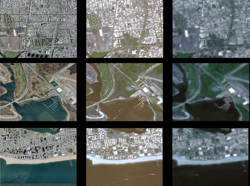
MACHINE LEARNING AND SATELLITE IMAGERY                         1

1.    Introduction

Artificial intelligence (AI) and machine learning are transforming every nook and cor-

ner of our world. In recent years, we have seen the emergence of calls for applying

AI and machine learning to solve socioeconomic, humanitarian, and environmental

problems from both the profit and nonprofit sectors. For example, in 2018, Google’s AI

for Social Good hosted the AI Impact Challenge, which awarded 25 million US dollars to

socially beneficial projects and organizations tackling global challenges (Google, n.d.).

Likewise, Microsoft, another tech giant, has launched a series of AI for Good initiatives

for empowering AI-equipped organizations to bring positive impacts via a pledge of

165-million-dollar financial support (Microsoft, n.d.). From the nonprofit side, the

United Nations (UN) has been advocating the promising role that AI can play to achieve

sustainable development goals through their annual AI summit (Butler, 2017). Accord-

ing to a report by McKinsey Global Institute (Chui et al., 2018), there are approximately

160 AI applications for social good, and they cover all 17 agendas for sustainable devel-

opment set by the UN.

     Among many applications of AI, the combination of computer vision and spatial

data have made remarkable advancement and shared the spotlight from both researchers

and practitioners. The growing applications of spatial data, such as maps and satellite

images on socioeconomic problems, can attribute to the technical breakthrough in

geographic information systems (GIS) and machine learning based on massive com-

puting power. Equally important has been the massive amount of data provision from

both the public and private sectors. Indeed, once generated and preprocessed for

third-party access, large-scale data have become readily available in almost real-time.

Moreover, with the assistance of crowdsourcing, big spatial data have been attached

to a variety of labels, changing many knotty problems to be solvable and an essential

component of training and evaluating supervised machine learning. Naik et al. (2017)

employed a computer vision method to the time-series street-view images with crowd-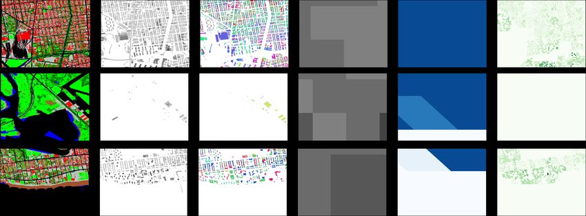
2                                      AHN ET AL.

sourced safety ratings to examine the physical dynamics of cities. High-resolution satel-

lite imagery, another primary source of spatial data, has been exploited in a convolu-

tional neural network to predict consumption and wealth at the local level (Jean et al.,

2016; Yeh et al., 2020).

   This paper presents how economists can integrate machine learning techniques

into satellite images to unearth economic measures more effectively from the view

above and to devise better economic policies. We first glance at how satellite imagery

has contributed to unraveling the traditional economics problems and will expand its

potential with the aid of machine learning in complementing the economics literature.

In particular, daytime, rather than nighttime, satellite imagery with high resolution is

our focus here. Subsequently, we introduce the current availability of both satellite

imagery and geographic ground-truth data. We also review the recent developments in

computer vision and image processing that can be of potential use in utilizing satellite

images and economic data. We then identify some of the challenges in teaching ma-

chines with satellite images as inputs and economic indicators as outputs: (1) defin-

ing economic labels, (2) data labeling to construct ground-truth, (3) lack of available

ground-truth economic data, (4) mismatch between district-level economic data and

grid-level satellite image data, (5) overfitting problem, (6) generalizability problem, and

(7) Black Box problem. Adding higher value is our suggested approach to these diffi-

culties and potential avenues for satellite imagery combined with machine learning in

future research.

   Satellite Data for Economic Research

Satellite imagery has never been so welcomed among the economics literature. Owing

to the recent development of computer vision algorithms, economists are collecting big

satellite data not just to explore novel questions but also to tackle questions that could

not be answered with traditional data sources. A comprehensive survey by Donaldson

and Storeygard (2016) has lowered the technical barrier to entry by providing a gentle

introduction to satellite data for economists and its applications. Over the past two
MACHINE LEARNING AND SATELLITE IMAGERY                          3

decades, however, satellite data sources utilized in much literature has mainly been

either luminosity from nighttime satellite images (i.e., night lights) or sensory data for

special purposes (e.g., ecological, meteorological, or topographical studies; for review,

see Donaldson and Storeygard 2016). Besides, despite the extensive coverage in both

time and space, prior studies often focused on a single country or area of interest only

at certain times.

   Nighttime Satellite Imagery as a Proxy for Economic Activity and Its Limitations

Nighttime satellite images or night lights are now a prominent, plausible proxy for

global and local economic activity; They have proven their versatility and robustness

in the economics literature. Gathered by US Defense Meteorological Satellite Program’s

Operational Linescan System (DMSP-OLS) and distributed by NOAA National Geophys-

ical Data Center, luminosity data are represented as a six-digit digital number (DN)

between 0 and 63 at a grid level; the higher the DN, the brighter the light radiance.

   Since the pioneering works by Chen and Nordhaus (2011) and Henderson et al.

(2012), night lights began to gain the attention and became a mainstream measure of

economic output, widely applied in a multitude of development economics research

(for review, see Michalopoulos and Papaioannou 2018). Recent papers have exploited

and verified the strong correlation between light density and output statistics at the

regional/within-country as well as global/cross-country levels (Chen and Nordhaus,

2011; Henderson et al., 2012; Pinkovskiy, 2017; Pinkovskiy and Sala-i Martin, 2016). In

addition to economic production, nighttime satellite imagery has been used to predict

energy consumption (Xie and Weng, 2016), epidemic fluctuations (Bharti et al., 2011),

regional favoritism (Hodler and Raschky, 2014; Lee, 2018), and urban growth in devel-

oping countries (Dingel et al., 2019; Michalopoulos and Papaioannou, 2013; Storeygard,

2016), even in areas without or lacking the reliable traditional measures.

   While night lights can be advantageous in measurement objectivity and wide spatial

and time-series coverage, they bare some drawbacks. Michalopoulos and Papaioannou

(2018) discuss several caveats of using luminosity at nighttime. The two most notable
4                                     AHN ET AL.

shortcomings are blooming and saturation. Blooming refers to the magnified light

emission from one pixel to adjacent pixels due to its reflection over some types (e.g.,

water- or snow-covered) of terrain. Saturation pertains to the top- or bottom-censored

values of DNs resulting from amplification for detecting highly bright or dim lights.

Because of these limitations, luminosity at night exhibits underperformance in areas

at the extreme ends of the wealth or income spectrum. Using relatively recent data

from the Visible Infrared Imaging Radiometer Suite (VIIRS), instead of DMSP-OLS, can

alleviate the blooming and saturation effects a little (Baragwanath et al., 2019). An

alternative solution to these limitations is the use of radiance-calibrated luminosity

data (e.g., Henderson et al., 2018).

   Advantages of Using Daytime Satellite Imagery and Applications in Economics

High-resolution daytime satellite imagery presents a raw picture of the world at a fine-

grained level, from which measures of human activities can be extracted directly. Day-

time satellite images are capable of capturing and offering more lavish features and pat-

terns observable from above compared to nighttime images. Although the accessibility

to high-resolution daytime satellite imagery goes way back, its frequent appearance in

the literature has only recently become possible due to the analytical complexity re-

sulting from high dimensions and lack of structures (Donaldson and Storeygard, 2016).

Thus, daytime satellite images at high resolution began to be utilized by leveraging the

high representation power of deep learning architectures.

   One popular usage of daytime satellite imagery is the land cover classification. Jay-

achandran et al. (2017) classified daytime images from QuickBird, a commercial satel-

lite with high-resolution support, and assessed the impact of Payments for Ecosystem

Services on (de)forestation in Ugandan villages. Similarly, Baragwanath et al. (2019)

detected urban markets by examining land covers from three different daytime satellite

datasets–including MODIS, GHSL, and MIX–based on supervised learning. Like the

night light examples, daytime luminosity can also be a unique proxy for socioeconomic

welfare, as shown in the recent study of Marx et al. (2019) on ethnic patronage among
MACHINE LEARNING AND SATELLITE IMAGERY                          5

informal settlements in Kenya.

     Notable advancement was made by Jean et al. (2016), who predicted poverty across

five African nations via a multi-stage approach called transfer learning. In their work,

transfer learning first trained a machine first to compare nighttime luminosity with

daytime pictures and then predicted consumption and wealth from daytime features

with the actual survey data. To the latest, Yeh et al. (2020) added more value to Jean et

al.’s (2016) finding by outperforming the extant model with analogous technique and

using only publicly available satellite data. One significant contribution that parallels

our attempts to be illustrated in later parts is their use of scarce labeled data, which

often hinders such prediction tasks.

     The remainder of the paper has the following structure: In Section 2., we discuss the

characteristics of geospatial data including satellite imagery and provide some acces-

sible sources in detail. In Section 3., we review the recent developments in computer

vision and image processing that can be applied to satellite images, and discuss several

challenges in using satellite images to teach machines to extract economic information

captured in satellite images. Section 4. describes our efforts to develop machine learn-

ing techniques that use daytime satellite images to measure economic development.

We also share our future research agenda and conclude in Section 5.

2.     Geospatial Data for Economic Research

2.1.    Satellite Imagery Data

The combined methods of machine learning and remote sensing highly depend on

satellite images. Satellite imagery datasets are stored in Raster formats, which are sets

of a large number of grid cells (or pixels) with corresponding values and geographic

coordinates. Satellite imagery datasets can be classified by diverse characteristics: or-

bits of satellite, resolution, and the numbers of spectral bands. Imagery is taken by

two-orbit satellites; geostationary satellites have orbits to continuously take images of a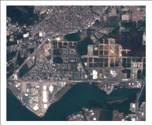
6                                      AHN ET AL.

fixed point, while sun-synchronous satellites have nearly polar orbits to keep the same

relational position with the Sun to capture any points of Earth.

   The Resolution of Satellite Imagery

The resolution of satellite images is described as a meter per pixel; however, as machine

learning techniques often use split individual images for analysis (e.g. (Jean et al.,

2016)), it is described with zoom level resolution in the field. Zoom level coordinate

system is based on how many 256-pixel wide tiles are used to divide the whole world.

As the system uses individual tiles, it is useful as input in deep learning models. Given

that zoom level 0 uses one tile to show the whole world, the tiles are split into four when

a zoom level goes up. The resolution of zoom level 15 is 4.773m per pixel, 16 for 2.387m,

and 17 for 1.193m. A popular example of the system is the Google Maps service. The

high-resolution satellite images (at most 5m resolution) are mostly used as daytime

imagery input in machine learning fields for predicting economic variables.

   The Spectral Bands of Satellite Imagery

Satellite sensors catch all wavelengths of the electromagnetic spectrum differently. Thus,

individually recorded wavelengths are referred to as spectral bands, and the number

of bands varies depending on the sensors. The bands include not only visible lights

of Red, Blue, and Green, but also other bands such as coastal aerosol, near-infrared

(NIR), water vapor, short-wave infrared (SWIR), and others. The combination of bands

can detect numerous types of human and natural objects; for example, Normalized

Difference Vegetation Index (NDVI) calculated by Red and NIR bands can measure the

state of plant health. However, machine learning studies to date tend to focus on Red,

Blue, and Green bands.

   The Cost of Satellite Imagery

The cost of satellite images depends on the resolution and size of the area. The high-

resolution datasets cost significantly up to USD 30/km2 ; selected examples of images

are Worldview 3/4 (30cm resolution), GeoEye 1 (40cm), KOMPSAT-3A (55cm), Quick-
MACHINE LEARNING AND SATELLITE IMAGERY                          7

               Figure 1: Publicly Available Satellite image, Brooklyn, NY.
                   Note: World Imagery (left), Sentinel2 (middle), Landsat8 (right)

bird (60cm), KOMPSAT 2 (1m), and SPOT 6/7 (1.5m). On the other hand, there are pub-

licly available datasets, including Landsat series (from 30m to 80m), Sentinel 2 (10m),

and World Imagery (on average up to 1.2m) via the REST APIs of Esri R ArcGIS (Johnston

et al., 2001). Landsat series are available from 1972, Sentinel 2 from 2015, and World

Imagery for the only one-time snapshot.

2.2.   Grid-level Ground-truth Data

For estimating economics with machine learning, it needs ground-truth data for train-

ing and evaluating the models. The primary approach is to use official district-level so-

cioeconomic statistics as ground-truth (Jean et al., 2016). In this approach, the world-

wide provided datasets such as Demographic and Health Surveys (DHS), are useful for

analyzing developing countries. However, district-level data have caveats as requiring

other grid-level supplementary data (e.g., nightlight data) corresponding to split indi-

vidual satellite images.

   Grid-level Ground-Truth Data Used to Date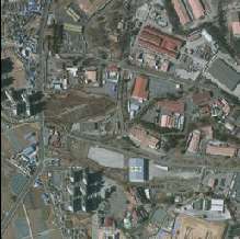
8                                        AHN ET AL.

Thus, there come various attempts to use grid-level data in recent studies. Hardly do

datasets provide official socioeconomic statistics at the grid level; raster datasets are

alternatively used to split into grids. Nightlight data is widely utilized (Jean et al., 2016).

Moreover, Han et al. (2020a) used Facebook humanitarian data for grid-level prediction

of population. Facebook has contributed by making the most precise population map

of the world, covering most of the Asian and African countries Facebook (2020). The

estimation is at the resolution of an arcsecond-by-arcsecond scale. Online geocoded

data, such as georeferenced Wikipedia articles, have also been used as proxies for so-

cioeconomic statistics (Fatehkia et al., 2018; Sheehan et al., 2019; Uzkent et al., 2019;

Rama et al., 2020).

   Other Possible Ground-Truth Data

There are several other possible grid-level data for proxies of economic activities. First,

among many digital elevation data, the Normalized Digital Surface Model (NDSM) is

useful in detecting human development at the grid level. Calculated by Digital Surface

Model (DSM) and Digital Terrain Model (DTM), NDSM displays the height of objects

over the surface. Thus, NDSM can show a total volume of human-constructed arti-

ficial objects in a given area. However, since digital elevation datasets are relatively

expensive, similar types of data, such as building footprint data, can be used as an

alternative. The building footprint data provide geospatial shapes of all buildings. It

is often provided by selected countries and publicly available from Openstreetmap

data (OSM). If footprint data is multiplied by floor levels of each building, it is the

gross floor area and similar to NDSM in concept. Third, the land use and land cover

(LULC) data describes the feature types of land, including vegetation, water, built-up,

and others. LULC can capture economic activities such as urbanization (built-up) or

agriculture (vegetation). LULC is diverse in terms of providers and class categories

based on geographical and national contexts, but there is also global-scale data such

as Copernicus Global Land Cover. Lastly, the land surface temperature (LST) describes

the radiative skin temperature of the land surface at day and night. Wang et al. (2018)
MACHINE LEARNING AND SATELLITE IMAGERY                                    9

            Figure 2: Examples of Grid-level Ground Truth Data, Brooklyn, NY.
Note: From left, (1) Landuse/landcover classification (NYC opendata), (2) NDSM (Digitalglobe), (3) Building
footprints(NYC opendata), (4) Nightlight data (NOAA), (5) Land surface temperature (MODIS), (6) Facebook
population data.

posed that patterns of LULC might have potential impacts on LST; the city core had

higher nighttime LST than rural areas, especially in cold seasons. LST data is publicly

available from MODIS.

2.3.   Reviews from a Data Perspective

The previous two sections examined satellite imagery and hyperlocal-level ground truth

data used in the field of machine learning in economics and remote sensing. However,

there are several caveats with utilizing the data. The predominant limit and tendency of

the previous approaches are to focus on high-resolution satellite images instead of low

and publicly available ones. As a result, few pieces of research have been conducted on

time-series analysis due to high costs. Moreover, the applicability of the study is low in

that the method to date cannot be easily followed. Although Yeh et al. (2020) posed the

possibility of using the public source, it is urgent to develop other machine learning

models for economic prediction with publicly available imagery with multi-temporal

data; Sentinel2 could be appropriate with a 10m resolution source from 2015. Second,

the satellite images cannot be interchangeably mix-used because they differ from each

other in terms of resolution, data type, color tones, degree of correction, the numbers
10 AHN ET AL.
of bands, coordinates, and other geographical metadata. This reduces the applicability
of models in which performance becomes lower with other sources of satellite imagery.
Third, as literature has been based on split individual tiles, the analysis inevitably takes
a great effort and time to clip massive raster data into smaller tiles. Although the World
Imagery dataset offers a clipped version of image tiles for users, other datasets need
to be split with tile extents. Lastly, there is no consensus on which hyperlocal or grid-
level data, beyond district-level statistics, should be used for ground truth of economic
activities. Research is needed to determine the most explanatory information among
various data sources suggested in the previous section.
3. Challenges in Teaching Machines to Read the Economic
Context of Satellite Images
3.1. Machine Learning for Satellite Image Processing
We have seen remarkable progress in teaching machines to recognize objects in an
image over the last decade. Machine learning models in computer vision and image
processing require a massive data set to train and test, and thereby enormous amounts
of computing power to process the data. Lack of such data had been the major hurdle,
but ImageNet (Deng et al., 2009), the large-scale crowdsourced data of labeled images,
sparked the fast growth of the technology. ImageNet has over 14 million images that are
organized according to nouns in the WordNet, a lexical database with the hierarchical
structure. With ImageNet, machines can be trained to learn what cats look like and
to distinguish them from other animals. The ImageNet Large Scale Visual Recognition
Challenge also has played a crucial role in serving as an incentive for researchers. The
state-of-the-art method as of May 2020 shows the top 5 accuracy rate of 98.7% – it
is only 1.3% of the time that machines’ top 5 guesses for the name of an object inMACHINE LEARNING AND SATELLITE IMAGERY 11
a presented image do not hit the right answer.1 This beats average humans as the
corresponding rate is about 95% for humans.
Generally speaking, object recognition can be divided into two tasks: object local-
ization and object classification. Object localization is to find a specific area, repre-
sented as a bounding box, in an image where an object resides. Object classification is
to find a label for an object in an image. Object detection is then the combination of
the two: detect an area where a specific object is contained and figure out the label for
the object.
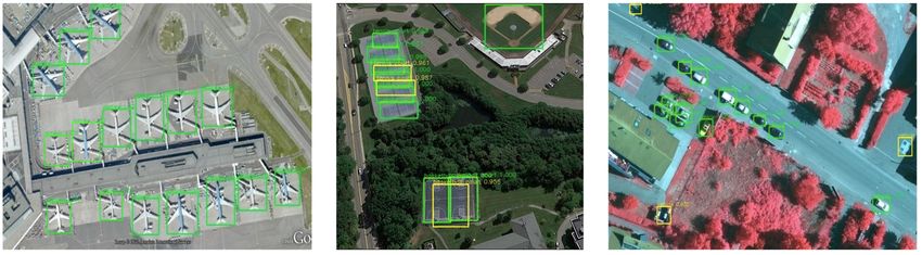
Object detection techniques to detect semantic instances, such as airplanes or cars,
have been widely applied to analyze satellite imagery (Wang et al., 2020; Chen et al.,
2014; Guo et al., 2018). In many cases, convolutional neural networks (CNN), a deep-
learning neural network algorithm, are first trained for object classification, and then
they are trained to draw a bounding box with ground-truth boundary data, where bound-
aries are marked by human annotation (See Figure 3) (Guo et al., 2018).
Figure 3: Object Detection in Satellite Images
Source: Guo et al. (2018)
While object localization and image classification can be regarded as basic tech-
niques, there are many other techniques in computer vision and image processing
that can be applied to analyze satellite images. Instead of object localization, which
1
https://paperswithcode.com/sota/image-classification-on-imagenet reports the most up-to-date
results.12 AHN ET AL.
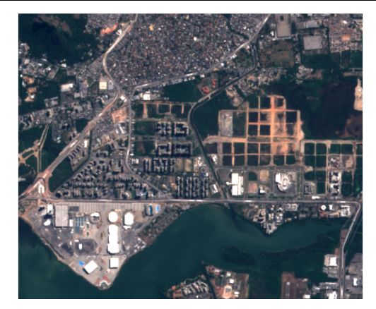
Figure 4: Satellite Image Data for Change Detection
(a) Rio on Apr 24, 2016 (b) Rio on Oct 11, 2017 (c) Ground-truth Change
Source: Daudt et al. (2018)
Note: The ground-truth change is annotated by humans.
draws bounding boxes, we may want to figure out the exact boundaries (or edges or
contours) of an object or some spatial instance. Or, one can take a pixel-based ap-
proach, such as in image segmentation. In image segmentation techniques, an image is
first partitioned into multiple semantic segments to generate sets of pixels with similar
characteristics. The algorithms then put a label on each set of pixels. In the end, every
pixel in an image will have a label (Chen et al., 2018). If the pixel level constructs LULC
data, it can be used to test the performance of image segmentation models. At the same
time, LULC data can be created by applying image segmentation.
As many economics questions involve growth or changes over time, detecting tem-
poral changes in satellite images can be of potential interest. What is essential in de-
veloping a change detection method is to define a change that we want to measure and
collect training data for such changes. Figure 4 shows an example of such data. Change
detection techniques were designed to detect the movement of buildings or changes
in terrain (Daudt et al., 2018) or to detect the long-term changes in the forest, while
ignoring other temporary changes such as clouds or other weather conditions (Khan et
al., 2017). These deep learning-based approaches either make a difference in high-level
features coming out of CNN layers, or train a CNN model using two images to compare
as input, and changes annotated by humans or administrative data as output.MACHINE LEARNING AND SATELLITE IMAGERY 13 3.2. Challenges While processing images to identify objects in them has been successful, processing satellite images and uncovering their economic information poses different challenges. Defining Economic Labels First of all, we do not yet have ImageNet for satellite imagery and economic informa- tion: while we have abundant satellite image data, we don’t have a set of economic labels that are readily available. To apply the currently available object recognition algorithms, we need to explicitly figure out what to teach: the ground truth for eco- nomic information by grid-level. Once the ground-truth data is available, we can teach machines that geographic characteristics captured in a satellite image are linked to the given economic information. The first step is then to define classes of labels, which represent economic infor- mation that can be captured in satellite images. With the defined economic labels and satellite images, we can formulate a classification machine learning problem. What could be the economic version of WordNet for satellite images? Objects that can be ob- served from satellite imagery, such as buildings, roads, airplanes, cars, and so forth, can serve as a class of labels. LULC and crop/vegetation categories can also provide a set of label classes. Taking an urban development perspective, ‘urban/rural/uninhabited’ la- bels can be helpful. Considering production side of an economy, ‘agriculture/manufacturing/ service/residential’ classification can also do a job. For each of these classifications, we may want to introduce a deeper hierarchy. For example, we can classify further ‘urban’- labeled images with ‘super-urban/urban/suburb.’ With these classifications, we can design a deep learning classification algorithm to assign a label to each satellite image. Data Labeling to Construct Ground-truth Labels The next step is to put a label to each satellite image, which requires human annotation. However, annotation can be costly in both time and money due to the massive size of satellite images and labeled data required to train and test. Therefore, many projects
14                                      AHN ET AL.

such as SpaceNet Challenges2 or Openstreetmap take a crowdsourced approach in col-

lecting labeled data. When adopting crowdsourcing, a design of labelling tasks for

efficiency and data validation for labeled data quality can be challenging.

   Lack of Available Ground-truth Economic Data

While addressing the classification problem can be useful, what is more relevant for

economic research is to put a number to each satellite image, which can be a measure

of economic activities such as population, consumption, wealth, inequality, poverty,

etc. This comes down to a regression task in machine learning with satellite images.

For example, we may want a machine learning algorithm to predict poverty from the

satellite images of a particular region.

   For this prediction task, economic statistics or administrative data at the grid-level

is required as the ground-truth to train and test the algorithm. The biggest challenge

is then the availability of such ground-truth economic data needed for cross-sectional

and time-series analysis. One solution we propose in Section 4.2.that can be applied

under absence of ground-truth data is redefining the task to predict relative economic

measures not absolute measures. We develop a deep learning technique which makes

use of economic labels and requires only lightweight human annotation to compare

different clusters of satellite images given some economic criteria. Our approach adopts

metric learning after classification and clustering tasks.

   Mismatch between District-level Economic Data and Grid-level Satellite Image

Data

While economic data is usually available by the administrative unit, satellite images

are stored in a grid format. This mismatch in representation makes existing models not

applicable to satellite images and district-level ground-truth: a district can be of any

polygon shape spreading over multiple satellite image tiles, which changes the input

dimension (the number of satellite images of the district) to the algorithm every time.
   2
       https://spacenet.ai/
MACHINE LEARNING AND SATELLITE IMAGERY 15 In Section 4.1., we propose a deep learning model to learn sophisticated spatial features of an arbitrarily shaped district based on high-resolution satellite images to produce a fixed-length representation of economic measures. Overfitting Problem When the size of labeled data is not big enough, a deep learning model may fit too closely or too exactly to a particular training dataset, which is referred to as the over- fitting problem. Overfitting leads models to lose generalizability and become less ap- plicable to other datasets. The lack of available ground-truth economic data and mis- match in representation, the previously discussed problems, make the overfitting prob- lem highly relevant in our context. Generalizability Problem Since some of geographic characteristics can be unique for each continent or for each country, designing a deep learning technique that are generally applicable is a difficult challenge. Moreover, some geospatial features contained in a satellite image can be affected by when the image was recorded, which aggravates the problem. There are two approaches we can take: either to develop a model that can transfer knowledge between different regions or to optimize a model for each region. We plan to test and expand generalizability as much as possible in developing deep learning models. Black Box Problem AI models, including deep learning, are criticized that prediction results from the mod- els are not interpretable or explainable, so called as Black Box problem of AI(Castelvecchi, 2016). The lack of interpretability and explainability prevents wider use of machine learning algorithms both in social science research and in practice despite its advan- tages. Making a model more interpretable and explainable is regarded as the most important and pressing challenge in the current literature. In our model presented in Section 4.2., we utilize some interpretable input to help explain the prediction result, which we believe one step towards tackling the problem.
16                                         AHN ET AL.

4.        Our Progress

In this section, we introduce our technical approach to solve some of the challenges

discussed in the previous section—mismatch in data representation and lack of avail-

able ground-truth economic data.

4.1.       Matching Grid-level Satellite Image Data to District-level Economic
           Data3

The existing machine-learning models are not applicable for predicting district-level

data. Since districts, unlike grids, can be of any polygon shape, this trait leads to a mis-

match when attempting to use satellite images with deep learning-based approaches.

TO overcome this, we propose a model that efficiently extract key fixed-length features

from any number of satellite images from an arbitrary region. Our method, called

Representation Extraction over an Arbitrary District (READ), utilizes daytime satellite image

tiles whose three vertices belong entirely to the polygon representing each district. A

single district can contain vastly different land covers such as urban built-up, water,

forest, etc. Our task is to learn these sophisticated spatial features of an arbitrarily

shaped district based on high-resolution satellite images to produce a fixed-length rep-

resentation of economic measures.

     READ is a lightweight method of measuring economic activities from high-resolution

images. The learned features are robust to the size of the original labels, such as pop-

ulation density, age, education, income, etc. We present a comprehensive evaluation

of the model based on a rich set of data from a developed country, South Korea, and

demonstrate its potential use in a developing country, Vietnam. The overall architec-

ture of READ is illustrated in Figure 5.4

     3
         This subsection is adapted from our work Han et al. (2020a).
     4
         The code is released at GitHub. https://github.com/Sungwon-Han/READ
MACHINE LEARNING AND SATELLITE IMAGERY 17
Pretrained CNN
cross-entropy
Labeled Images Student network
Custom Dataset(4) classification cost weighted
Exponential
Moving Average
sum
mean squared
CNN error (MSE)
total cost
Resnet-18 (B) consistency cost
Unlabeled Images Teacher network (step1)
(step2) (step3)
fine-tuned
&' PCA &' ′
(reduced dimension : 1)
CNN &( *!× .'( &( ′
∈, ∈ , *!× 0
⋮ ⋮
Resnet-18 (A) &*!
Images from &*!′
district dataset !(#$ )
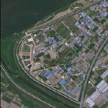
:18 AHN ET AL. a given input, and it can be extracted from network’s hidden layer. To train the network with its embeddings, we constructed a labeled custom dataset (C) that includes 1,000 randomly selected satellite images and employed the following three labels directly related to a degree of urbanization: urban, rural, and uninhabited. We hired four an- notators to obtain the labels of the images. We integrated all annotators’ decisions as soft labels (i.e., average votes), which were then used to build a classifier that divides satellite images into three classes. However, obtaining reliable labels for each satellite image tile was a time-consuming task. Here, a key challenge was the relatively small number of labeled data, which was addressed by adapting a semi-supervised learning approach. Semi-supervised learning aims at training classifiers based on a small amount of labeled data and a large amount of unlabeled data. Mean Teacher (Tarvainen and Valpola, 2017), which is a powerful model in this domain, utilizes unlabeled data to pe- nalize predictions that are inconsistent between the student and teacher models. This regularization technique can provide smoothing in the decision boundary for a robust and accurate forecast. We used the Mean Teacher architecture with the ResNet18 back- bone for training. In addition to semi-supervised learning, we concurrently adopted transfer learning. Transfer learning is a learning technique that utilizes knowledge from another dataset to solve the main task. Knowledge gained from a similar dataset helps efficient training and prevents the model from overfitting. Following the idea, we first pretrained the CNN model with the ImageNet dataset (Deng et al., 2009), and then use the pretrained model as an initial student network in the Mean Teacher model. To determine whether the trained classifier extracts essential features, we visualized sample images into three-dimensional space by reducing the embedded vectors by PCA. Figure 6 displays the extracted features in the reduced vector space of sample images of various urban and rural areas. Here, the rural and urban images are separated and aligned well in the virtual direction (i.e., red and blue arrows). Furthermore, these virtual axes represent the degree of urbanization. The left-hand side of the picture
MACHINE LEARNING AND SATELLITE IMAGERY 19
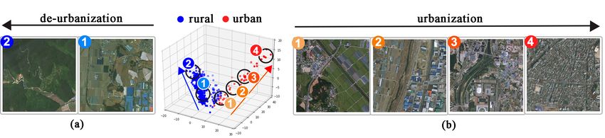
Figure 6: Graphical Representation of an Embedded Space: Urban vs. Rural
Note: This embedded space analysis shows that rural images (blue) are well separated from more urban
images (red). For the blue cluster, as we observe images from anchor points 1 to 2, the de-urbanization
trend becomes more pronounced. In contrast, for the red cluster, as we observe images from anchor points
1 to 4, the degree of urbanization becomes more intense.
shows two satellite image tiles. Both tiles have rural characteristics, and the images
that seem to contain a smaller human population are positioned further toward the
blue arrow (i.e., tile “2” seems less urbanized than tile “1”). The image tiles on the
right-hand side contain capture more populated areas. Tiles “3” and “4” that are toward
the end of the red arrow show a highly urbanized cityscape, whereas tiles “1” and “2”
contain fewer residential areas. This figure demonstrates the strength of our model in
its ability to learn high-level features and align satellite images along these virtual axes.
Data Pruning
According to the Global Rural-Urban Mapping Project, only 3% of the land cover is an
urban area, and approximately 40% of the land is an agricultural area (Doxsey-Whitfield
et al., 2015; Foley et al., 2005). The remaining uninhabited area accounts for the most
considerable portion of the earth. Since such regions do not show human artifacts,
they could act as noise when extracting representations related to human activities. We
built a CNN classifier by filtering areas that are probably uninhabited. For the training,
we reused a custom dataset that included 1,000 randomly selected satellite images. Of
the initial 96,131 images, 51,618 (53.702%) images were removed in this manner.
Dimensionality Reduction of Embedding20 AHN ET AL. The next step reduces the dimensions from the final layer in ResNet18 into smaller sizes. Since our goal is to predict attributes of interest yi and obtain a unique rep- resentation from a pruned image set D̂i across districts (i.e., n = 230 administrative districts), we aimed to produce a dimension size vi smaller than the number of districts n to avoid overfitting. We implemented a principal component analysis (PCA) to reduce the dimensions of the embedded features vi , which appears in the center of Figure 5. Presenting the Embedded Spatial Statistics This final step addresses the challenge arising from the varying input size in which a different number of image tiles define districts. Previous studies in a different do- main have attempted to address such arbitrary input length problems via preprocess- ing techniques, such as adding sequence padding or recurrent neural network-based learning (Yang et al., 2016; Hochreiter and Schmidhuber, 1997). However, these meth- ods cannot resolve the substantial differences in input lengths typical in demographic research. The smallest district could be covered by fewer than ten image tiles, whereas the largest district requires more than hundreds of tiles, resulting in orders of magni- tude difference. We present a technique to summarize any length of image features into a fixed set of vectors. Let g be the composition of the fine tuned feature extractor and k (1 ≤ k ≤ 10) be the resulting principal components. All images dij in D̂i are transformed to vj0 ∈ Rk by g. Let the matrix of the final embedded vectors from district i be Ri ∈ Rni ×k . To produce a fixed-length embedding from vast geographic areas, we propose to utilize the following descriptive statistics: (i) the mean µ, (ii) the standard deviation σ, (iii) the number of satellite images of a district n, and (iv) Pearson’s correlation of the dimensionally reduced features ρ. These four quantities are fundamental embed- ded spatial statistics capturing the observation that satellite images of areas with geo- proximity exhibit similar traits. Descriptive statistics represent data by central tendency (mean, median, and mode), dispersion (variance, standard deviation, and skewness), and association (chi-square and correlation). The proposed quantities are descriptive
MACHINE LEARNING AND SATELLITE IMAGERY                        21

statistics representing satellite images that belong to the same district.

   Finally, cross-products of features were added to consider interactions to enrich the

information regarding unknown embedded space distributions. These complete sets

of features were learned per district i, as illustrated in the bottom part of Figure 5 and

became a fixed-sized representation ri . To predict the yi value for district i, we used ri

to fit a regressor.

4.1.2.   Data

This study utilizes the following data: regional-level demographics and high-resolution

World Imagery satellite images. We chose South Korea as a representative developed

country for training the model. Then, among all available satellite images of South

Korea, we further identified those in which at least three vertices of an image tile belong

to the polygon representing the boundaries of each district. This heuristic is simple

but reasonable for addressing various polygon shapes. In total, 96,131 satellite images

(256 × 256 pixels) of 230 South Korean districts were collected this way. The utilization

of all image tiles per district distinguishes our work from those of others, c.f., previous

studies used a fixed set of satellite images. For example, a seminal study conducted in

African countries used 100 randomly chosen image tiles over 10x10 km2 areas (Jean et

al., 2016).

4.1.3.   Results

    Performance Evaluation and Ablation Study

We conduct a set of experiments. The first evaluation takes advantage of the population

demographics by dividing these data into a training set and a test set in an 80–20 ratio.

4-fold cross-validation is applied to the training data set to tune the model’s hyperpa-

rameters, such as the PCA dimensions and the regularization term in the cost function.

   We implemented nine baselines to evaluate. Nightlight uses the districts’ total light

intensity from nighttime satellite imagery to predict economic scales (Bagan and Yam-
22 AHN ET AL. agata, 2015). A regressor was built and trained to obtain the sum of nightlights in each district. Then, Auto-Encoder extracts compact features as step-2. An autoencoder is an unsupervised deep learning algorithm that does not need any label information. The model aims to learn an approximate identity function to construct an output similar to the input while limiting the number of hidden layers. No-Proxy is identical to the proposed model but lacks any knowledge transfer from the proxy dataset. This model was pretrained only with the ImageNet dataset and, hence, can demonstrate the value of the custom dataset. To verify the effectiveness of READ compared to a well-known model (Xie et al., 2016), we trained JMOP (Jean Model with Our Proxy) which is a combination of two models. First, we use a proxy that predicts rural, urban, and inhabited classes in the same method of READ. Then, we summarize the features and use them to predict with an identical set of model (Xie et al., 2016). Finally, SOTA is the best known grid-based approach for population density prediction (Facebook, 2019). The implementation details of this model are not published, but the prediction results on each arc second block (approximately 30 × 30 m2 ) are shared online. We could aggregate the published grid-level data across districts and regress such data with ground truth statistics. The four remaining baselines are ablation studies that remove each feature from READ. All models were trained with an 80–20 train-test ratios and 4-fold cross-validation. XGBoost (Chen and Guestrin, 2016) was used to enhance prediction accuracy. The models were evaluated 20 times with a randomly split dataset. Table 1 reports the mean and standard deviation of the predictions. READ outperforms all of the nine baselines in both the R-squared (R2 ) and mean squared error (MSE) values. Our model even outperforms the current state-of-the-art (SOTA) approach, which is (Facebook, 2019). We find that transfer learning from the custom land cover dataset helps produce a more meaningful embedded, by distilling knowledge associated with urban and rural classifications. The increased prediction quality demonstrates this finding against two models: No-Proxy and Auto-Encoder.
MACHINE LEARNING AND SATELLITE IMAGERY                            23

          Table 1: Model Prediction Performance Results and Ablation Study

                        Model                MSE              R-Squared
                    Nightlight         0.4254±0.0664        0.6133±0.0635
                    Auto-Encoder       1.6242±0.3445        0.6347±0.0823
                    No-Proxy           0.2800±0.1118        0.7359±0.1117
                    JMOP               0.4448±0.0998        0.8985±0.0253
                    SOTA                       -            0.9231
                    READ w/o µ         0.2612±0.0632        0.9429±0.0155
                    READ w/o ρ         0.2165±0.0596        0.9527±0.0140
                    READ w/o n         0.1921±0.0471        0.9579±0.0119
                    READ w/o σ         0.1902±0.0592        0.9586±0.0130
                    READ              0.1761±0.0383         0.9617±0.0090

          Note: The performance tests were made for prediction of population density.

   Furthermore, the quality gain over JMOP indicates that the summarizing technique

of READ contributes massively to the performance gain. We perform ablation study

to examine the importance of our model components. Ablation study refers to the

analysis that removes a particular component of the model, and investigates how that

affects the overall performance. The ablation study shows that removing any of the

descriptive statistics lowered the performance, indicating that n, µ, ρ, and σ all make a

meaningful contribution.

   Evaluation Over Broader Scales and Countries

The final evaluation reports predictions of a set of socioeconomic measures by READ.

All values are log-scaled, and XGBoost is used. The average R2 of 20 trials of prediction

of the study area is shown in Table 2. The second column shows precise predictions of

READ applied to South Korea to predict the population density and its subclass divided

by age groups (R2 > 0.95). Predictions on income per capita are 0.76 for R2 . Finally,

two demographics in the household category show an extreme difference in their pre-
24 AHN ET AL.
diction quality: While the household count per square kilometer reports the highest
R2 of 0.9664, the average household size reports the lowest R2 , i.e., 0.6181, among the
socioeconomic measures.
Table 2: Prediction Performance for South Korea and Vietnam
Target variable South Korea Vietnam
Population density 0.9617 0.8863
Population density by age 0-14 0.9520 0.8756
Population density by age 15-29 0.9570 0.8791
Population density by age 30-44 0.9575 0.8881
Population density by age 45-59 0.9624 0.8804
Population density by age 60+ 0.9654 0.8731
Household count 0.9664 0.8896
Household size 0.6181 0.4460
Income per capita 0.7603 0.6822
Note: The highest R2 value for each country is highlighted in bold.
The high prediction capability of READ may be due to the custom dataset, which
was built from the same country (see step-1 in Figure 5). To test its applicability to
another country, Vietnam, we gathered a total of 226,305 satellite images along with its
socioeconomic measure data. Then, we applied the model learned from South Korea
to predict the socioeconomic measures of Vietnam. Table 2 shows the prediction re-
sults. Predictions on population densities show surprisingly high R2 values, averaging
at around 0.88. This is despite the model being trained solely on data from a different
country.
The results from the above exercise demonstrate that the learned spatial representa-
tion of READ successfully captures general indicators of socioeconomic measures that
extend beyond a single country use. However, it is plausible that the strikingly high
prediction performance across South Korean and Vietnam is because both countries
exhibit similar pathways in economic growth and demographic transition (McNicoll,MACHINE LEARNING AND SATELLITE IMAGERY 25
2006).
4.2. Measuring Economic Development Under Absence of Ground-truth
Data5
To overcome the lack of economic data to be used as ground-truth, we developed a
deep learning model that learns from high-resolution satellite images to rank relative
scores of economic development without any labeled data. Specifically, we apply metric
learning to score relative economic activities, which avoids the use of ground-truth
economic data. Metric learning aims to define a task-specific metrics in a supervised
manner from a given dataset. Our metric learning algorithm learns to score satellite
images for the relative level of economic development measured by urbanization. Our
deep neural network first clusters images based on visual features and then defines
ordered and paired sets of clusters, i.e., a partial order graph (POG). The POG, an in-
put to the metric learning, contains the information on whether a specific cluster is
more urbanized than each of the other clusters. Trained with the constructed POG, our
algorithm assigns a score to each satellite image in the final step.
The POG is an essential element in our approach, addressing the limitations of the
existing methods. First, since a POG can be generated either by readily available data
or by light human annotation, our model can be applied to the cases without labeled
data. That is, our model can be used both for developing economies where labeled
data is limited and for developed economies where grid-level census data are not gath-
ered frequently. Second, since the POG is an interpretable input to our deep learning
algorithm, it helps us to understand the final scores that the algorithm produces. We
believe our approach makes one step toward resolving the Black Box problem.
Our model operates in three stages. The first stage (siCluster) uses an entire collec-
tion of satellite images of a target country and clusters them by a deep learning-based
unsupervised learning and transfer learning. siCluster uses labels for the general land
5
This subsection is adapted from our work Han et al. (2020b).26 AHN ET AL.
cover types, such as rural, urban, and uninhabited. The second stage (siPog) builds
a POG of the clusters from siCluster. The order of a POG captures the relative level of
economic development, for which we use urbanization as a comprehensive proxy, fol-
lowing the economics literature (Henderson, 2003). Two different methods to generate
a POG are suggested: the clusters are ordered either by humans (human-guided) or by
data such as population density or nightlight intensity (data-guided). Lastly, the final
stage (siScore) uses the POG from siPog to assign a differentiable score, via a CNN-based
model.
The proposed computational framework to measure sub-district level economic
development from satellite imagery without the guide of any partial ground-truth data
is novel and shows remarkable performance gain over existing baselines. Codes and
implementation details are made available at the project repository.6
4.2.1. Model Overview
Problem definition: Let I = {x1 , x2 , . . . , xn } be the set of satellite images
for a given area. The main goal of the proposed model f is to compute a
score ŷi for each image xi (i.e., ŷi = f (xi )) that well represents the economic
development level yi . We assume ground truth values of yi are unknown at
the training phase.
As a solution, we propose a weakly-supervised method to estimate relative scores
that highly correlate with the target variable yi , rather than predicting its absolute val-
ues directly. The method consists of three steps, which are described in Figure 7.
4.2.2. Clustering Satellite Imagery with siCluster
To generate scores that represent the urbanization level, one needs to know what kinds
of human activities capture such values. For distinguishing various human activities
6
https://github.com/dscig/urban_scoreMACHINE LEARNING AND SATELLITE IMAGERY 27
Rural Urban
Scoring
Model
0.1 0.3 0.9
Maximize Spearman with POG
Collect satellite images Predict urbanization
(a) siCluster (b) siPog (c) siScore
Figure 7: The Model Overview
Note: The overall architecture of the proposed model, composed of (a) siCluster for clustering satellite
images, (b) siPog for generating partial order graph (POG), and (c) siScore for training the scoring model
with POG.
from satellite imagery, we adopt DeepCluster (Caron et al., 2018), the deep learning-
based clustering that can efficiently handle the curse of dimensionality problem via
hierarchical architectures (Goodfellow et al., 2016; Krizhevsky et al., 2012).
DeepCluster has two limitations. One is the initial randomness; the model is af-
fected by the initial weights that can propagate through the training process. Another
is the lack of consistency in the class assignment; the model relies on the pseudo-labels
generated from its k-means clustering, subject to noise in data. As a result, DeepCluster
is not directly applicable to our problem, and the satellite grids are grouped according
to trivial traits such as RGB patterns (Caron et al., 2018; Ji et al., 2019). Our clustering
algorithm, siCluster, builds upon DeepCluster with two new improvements.
Improvement #1 from transfer learning: To give a good initial point for the encoder,
we constructed a labeled dataset for transfer learning that includes one thousand satel-
lite images with three labels: urban, rural, and uninhabited. We then adopted a semi-
supervised learning technique to train the classifier over the small set of labels and
massive amounts of unlabeled data. The Mean Teacher (Tarvainen and Valpola, 2017)
model, which penalizes the inconsistent predictions between the teacher and student,
is used.
Improvement #2 from consistency preserving: We added new loss terms to prevent
the model from learning trivial features. Suppose a given satellite grid xi and its cor-
responding encoded vector vi , i.e., vi = hW (xi ). We then augment xi via common28 AHN ET AL.
techniques such as rotation, gray-scale, and flipping that do not deform the original
visual context. Let us call the augmented versions x̂i . Then, the distance between xi
and its augmentations x̂i in the embedding space should be close enough, compared
with the distance between xi to other data points. We define the consistency preserving
loss to represent this invariant feature characteristic against data augmentation in the
embedding space. siCluster is trained by jointly optimizing the negative log-likelihood
loss and reducing the Euclidean distance between the input and its augmentations on
embedding space (Eq. 1).
1 X
Lecp = || hW (xi ) − hW (x̂i ) ||2 (1)
|B|
i∈B
4.2.3. Constructing Partial Order Graph with siPog
Images within each cluster share similar visual contexts that likely represent a similar
level of economic development. The second step of the algorithm aims at ordering
these identified clusters. The partial order graph (POG) is an efficient representation
showing the order across different clusters while ignoring any within-cluster difference.
We generated a POG in the order of economic development. Here, development refers
to an economic transition from agriculture to manufacturing and service industries,
which tend to cluster in more urbanized areas (Henderson, 2003). When two clusters
showed a similar level of development, they were placed at the same level without
any strict ordering between them, as illustrated in Figure Figure 7(b). Below are two
strategies of siPog.
Human-guided Method
We first considered the human-in-the-loop design and asked human annotators to
sort clusters manually. Both experts and laypeople participated in this ordering task.
Annotators compared clusters and identified relative orders of clusters by examining
the provided grid images. Clusters were ordered and connected as a graph by their
presumed economic development level. Cluster pairs whose development levels wereMACHINE LEARNING AND SATELLITE IMAGERY 29 judged to be indifferent were placed at the same level within the POG. The strength of this method is its lower cost than the full comparison of images. Data-guided Method POG can also be generated without human guidance. While grid-level demographics are costly to obtain, there are ample resources that can be used as a proxy, such as Internet search results. Proxy data are aggregated at a high-level (e.g., city or province) or are not accurate. Below we demonstrate one example, nightlight luminosity. Nightlight luminosity is the light intensity measured in nighttime satellite imagery. This publicly free data is only available at low resolution. We first extrapolate the night- time images to match the size of the daytime satellite grids. Once we identify all the extrapolated nighttime grids corresponding to each cluster, nightlight intensity was averaged for each cluster. We perform a two-sample t-test with a threshold 0.01 to detect any significant intensity difference between every two clusters and consequently create an edge between them if two clusters are sufficiently comparable. 4.2.4. Computing Scores with siScore Now given the relative orders of clusters in the POG, the next task is to assign a score between 0 and 1 to every cluster using the CNN-based scoring model f . The model automatically detects which features of satellite imagery (belonging to clusters) deter- mine the urbanization score via supervised learning. We adopt the list-wise metric learning method with our unique structures for the scoring model, siScore. During training, we limit the range of values of the scoring model from 0 to 1 by clamping smaller or larger values. List-wise Metric Learning The only knowledge from POG is the orders of clusters, but not the orders of individuals images. The third step, siScore, use the POG structure in learning scores of every satellite grid in the following way. We first extract every ordered path from the POG. After choos-
You can also read