WP/20/1 Debt Is Not Free - International ...

WP/20/1

 Debt Is Not Free

 by Marialuz Moreno Badia, Paulo Medas, Pranav Gupta, Yuan Xiang

IMF Working Papers describe research in progress by the author(s) and are published
to elicit comments and to encourage debate. The views expressed in IMF Working Papers
are those of the author(s) and do not necessarily represent the views of the IMF, its
Executive Board, or IMF management.

© 2020 International Monetary Fund WP/20/1

 IMF Working Paper

 Fiscal Affairs Department

 Debt Is Not Free

 Prepared by Marialuz Moreno Badia, Paulo Medas, Pranav Gupta, Yuan Xiang1

 Authorized for distribution by Catherine Pattillo

 January 2020

 IMF Working Papers describe research in progress by the author(s) and are published to
 elicit comments and to encourage debate. The views expressed in IMF Working Papers are
 those of the author(s) and do not necessarily represent the views of the IMF, its Executive Board,
 or IMF management.
 Abstract
With public debt soaring across the world, a growing concern is whether current debt levels are a
harbinger of fiscal crises, thereby restricting the policy space in a downturn. The empirical evidence to
date is however inconclusive, and the true cost of debt may be overstated if interest rates remain low. To
shed light into this debate, this paper re-examines the importance of public debt as a leading indicator of
fiscal crises using machine learning techniques to account for complex interactions previously ignored in
the literature. We find that public debt is the most important predictor of crises, showing strong non-
linearities. Moreover, beyond certain debt levels, the likelihood of crises increases sharply regardless of
the interest-growth differential. Our analysis also reveals that the interactions of public debt with inflation
and external imbalances can be as important as debt levels. These results, while not necessarily implying
causality, show governments should be wary of high public debt even when borrowing costs seem low.

JEL Classification Numbers: E43, E62, F34, F37, H63

Keywords: crisis, debt, default, fiscal, machine learning

Author’s E-Mail Address: MMorenobadia@imf.org, PMedas@imf.org, PGupta@imf.org,
YXiang@imf.org

1
 We are indebted to James Feigenbaum, Catherine Pattillo, Shuyi Liu, Nobuo Yoshida, Kazusa Yoshimura,
participants in the 8th annual workshop on Fiscal Policies and Institutions organized by the IMF in Brussels, and
colleagues at the IMF for useful comments. Juliana Gamboa Arbelaez, Ade Adeyemi, and Kadir Tanyeri
provided excellent research assistance and support with coding.

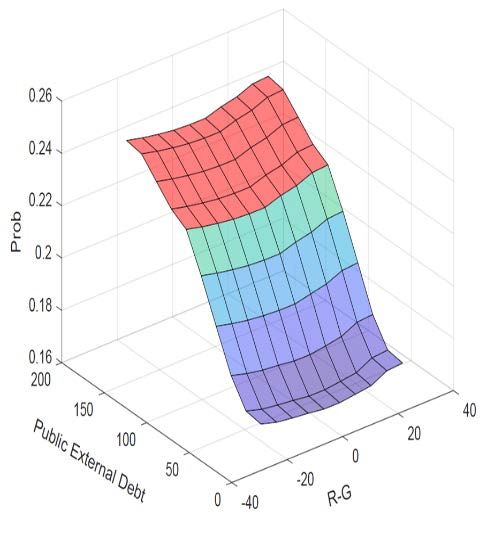
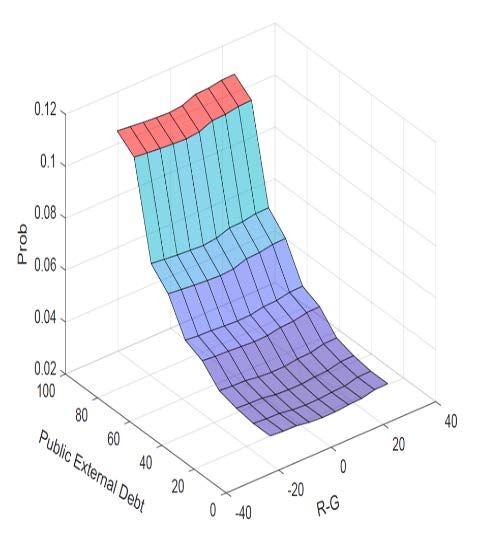
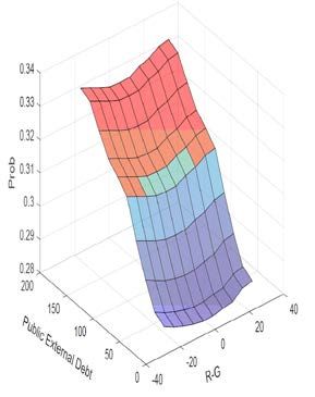
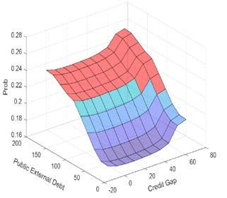
3

 Contents Page

I. Introduction ............................................................................................................................5

II. Does Debt Matter? Lessons from the Literature ...................................................................7

III. Data ......................................................................................................................................9
 A. Measuring Fiscal Crises ............................................................................................9
 B. Predictors .................................................................................................................11

IV. Methodology ......................................................................................................................13
 A. Variable selection ....................................................................................................14
 B. Assessing variable importance ................................................................................16
 C. Studying interactions and nonlinearities .................................................................16

V. Results .................................................................................................................................17
 A. Variable selection ....................................................................................................17
 B. Variable importance ................................................................................................19
 C. An analysis of selected predictors ...........................................................................20

VI. Conclusion .........................................................................................................................23

References ................................................................................................................................25

Tables

Table 1. Fiscal Crises Episodes (1980–2016) ..........................................................................11
Table 2. Out-of-Sample Performance of Alternative Feature Selection Algorithms...............18

Figures

Figure 1. Predictors of Fiscal Crises in the Literature .............................................................34
Figure 2. Most Common Predictors in the Literature ..............................................................34
Figure 3. Countries with Fiscal Crises, 1980–2016 .................................................................35
Figure 4. Overlap with Other Crises, 1980–2016 ....................................................................35
Figure 5. Debt Statistics: Country Coverage, 1980–2016 .......................................................35
Figure 6. Public and Public External Debt, 1980–2016...........................................................36
Figure 7. Interest-Growth Differential, 1980–2016 .................................................................36
Figure 8. Feature Selection Algorithms ...................................................................................37
Figure 9. Robustness in Variable Selection .............................................................................37
Figure 10. Variable Importance by Group of Predictors .........................................................37
Figure 11. Contribution to Probability of a Crisis ...................................................................38
Figure 12. Partial Dependence Plots1/ and Event Studies .......................................................39
Figure 13. Overall Interaction Strength ...................................................................................40
Figure 14 Top-10 Interactions with Public ..............................................................................40
Figure 15. Bivariate Partial Dependent Plots: Public External Debt and r-g...........................40
Figure 16. Inflation: Univariate Partial Depedence Plots ........................................................41

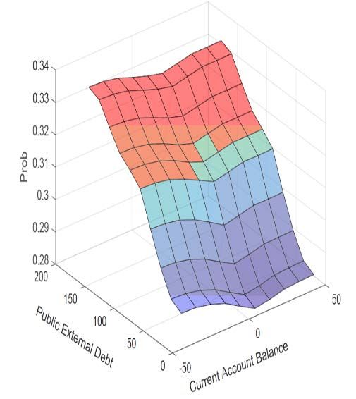
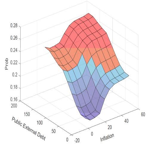
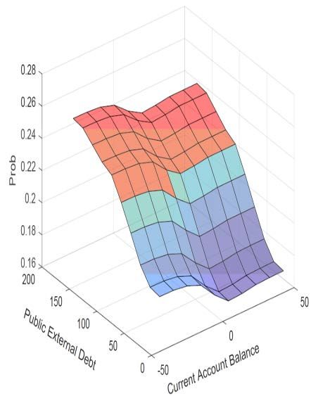
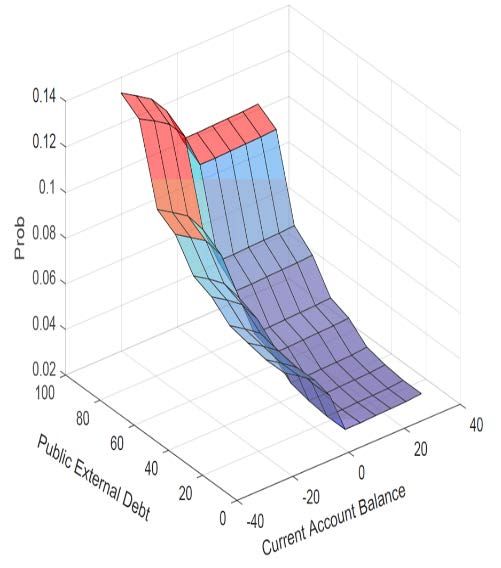
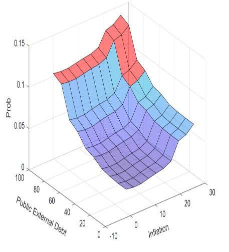
4

Figure 17. Inflation and Public External Debt: Bivariate Partial Dependence Plots ...............41
Figure 18. Current Account: Univariate Partial Dependence Plots .........................................42
Figure 19. Current Account and Public External Debt: Bivariate Partial Dependence Plots ..42
Figure 20. Credit Gap: Univariate Partial Dependence Plots ..................................................43
Figure 21. Credit Gap and Public External Debt: Bivariate Partial Dependence Plots ...........43

Appendixes

1. Literature Review.................................................................................................................44
2. Fiscal Crisis: Definitions and Data Sources.........................................................................51
3. Sample of Countries .............................................................................................................52
4. Data: Definition, Sources, and Predictor Groupings ...........................................................53
5. Methodological Details ........................................................................................................64

Appendix Table 5.1. Out-of-Sample Performance ..................................................................67

5

“Economic ruin admits of varied interpretations, but most of them apply at present to the greater part of
Europe, and most of the ruin is to be ascribed to the piling up of debt”

 J. S. Nicholson, “Adam Smith on Public Debts,” The Economic Journal, 1920

 I. INTRODUCTION

Should governments worry about high public debt? The answer from standard debt
sustainability frameworks is yes, for not only does real economic growth dip in the
immediate aftermath of a fiscal crisis, but the loss of output is often permanent (Medas et al.
2018; Asonuma et al. 2019). However, despite Reinhart and Rogoff’s (2009 and 2011a)
seminal work on the perils of excessive debt, the empirical literature on the relationship
between public debt and fiscal crises is still surprisingly inconclusive to this day. The case
for more public debt is being reinforced by weak economic activity across the globe, large
investment needs, and increasing concerns that monetary policy may be reaching its limits
particularly in advanced economies. And yet, the risk of fiscal crises still casts a long
shadow. Therefore, as many countries remain riddled with mounting debt, one of the most
pressing questions facing policymakers is whether current high debt levels are a bellwether
of future crises with large economic costs.

The argument that “public debt may have no fiscal cost” (Blanchard 2019) is also gaining
traction as many countries face historically low interest rates and the global stock of
negative-yielding debt is hovering around $12 trillion by the end of 2019. The underlying
rationale is that if interest rates are lower than the economic growth rate—that is, the interest-
growth differential is negative—there is no reason to maintain a primary surplus as it would
be feasible to issue debt without later increasing taxes.

To help shed more light on this debate, we use machine learning models to identify robust
predictors of fiscal crises and ask whether public debt is a reliable leading indicator by itself
or when interacting with other variables. The lack of strong evidence on the importance of
public debt stems from various methodological challenges. First, not only are crises rare
events but also limitations with debt data make robust modelling difficult. 2 More
importantly, it is very hard to distill complex nonlinearities and interactions from the classic
econometric techniques typically employed in the early warning literature. Namely, the debt
dynamics depend on many factors (e.g. interest rate, growth, deficit, shocks) and some of
those interact with each other: for example, a government may respond to a period of a low
interest-growth differential by increasing the deficit—which may in turn lead to higher debt
and increase the risk of a crisis. Therefore, with few settled facts, the debate on whether

2
 In the aftermath of the global financial crisis, several scholars compiled new panel datasets on debt covering
many decades (if not centuries) of data—e.g. Reinhart and Rogoff (2009) and Abbas et al. (2011) on public
debt; and Jordà, Schularick, and Taylor (2016) on private debt. Unfortunately, these datasets tend to include
only a few countries or use a narrow and changing definition of debt limiting the scope of research.

6

public debt matters for predicting fiscal crises remains unresolved. Our paper takes a step
toward filling that gap.

We bring evidence to bear on the issue by studying fiscal crises in a broader sample (188
countries) than previously used in the literature going back to the 1980s. One of the main
novelties of our empirical strategy is to take an agnostic approach to the selection of
predictors following a two-step procedure. As a starting point, we consider a wide range of
predictors, including covariates that the literature commonly associates with the onset of
crises. Also, we do not take a view as to what the relevant moments of the variables are but
instead consider many permutations yielding a total of 748 indicators. By leveraging machine
learning models, we can fit complex and flexible functional forms to our data without
overfitting. Our objective, however, goes beyond obtaining a well-performing prediction
model as we also want to identify those variables enabling that good prediction. Thus, in a
second step we reduce the large set of predictors to the ones that contain more information
than noise by using what is referred to in the machine learning literature as “feature
selection”. We then use a battery of statistical measures to go beyond the black box, allowing
us to uncover the relative importance of variables and their interactions.

Our results show public debt in its various forms is the most important group of predictors.
This finding is not an exclusive feature of the period immediately predating the global
financial crisis but applies more broadly. The narrative, however, is far from simple as some
forms of debt are more important than others—in particular, public external debt—and there
is strong evidence of non-linearities across all income groups. Remarkably, the interest-
growth differential has low predictive value. What is more, beyond certain debt levels the
likelihood of fiscal crises increases significantly irrespective of whether the interest-growth
differential is highly positive or negative. Event studies give some insights as to why this
may be the case: it is only at the onset of the crisis that the interest-growth differential spikes,
making it immaterial for signaling purposes. Our empirical analysis also reveals that it is not
solely public debt that matters as its interactions with other variables are as important. Hence,
the probability of a crisis rises steeply at high public debt levels but also at relatively
moderate ones when accompanied by high inflation or large current account deficits.
Notably, these results hold across all income groups.

Our work is related to the extensive early warning literature on sovereign debt crises (see, for
example, Detragiache and Spilimbergo 2001; Manasse, Roubini, and Schimmelpfennig 2003;
and Chakrabarti and Zeaiter 2014). Relative to that literature, our contribution is twofold.
First, we analyze systematically the predictive importance of public debt thanks to a more
comprehensive dataset on debt and its characteristics (such as the creditor structure) than
previous studies and an unparalleled number of macro indicators. To the best of our
knowledge, this is also the first study to examine explicitly the predictive power of the
interest-growth differential. The use of a much broader sample enables us to explore the
sensitivity of our results along the time and country grouping dimensions. As an additional
layer ensuring robustness, we assess the performance of alternative algorithms not only in

7

terms of the out-of-sample predictive accuracy but also the stability of the variable selection
with respect to sampling variation. Our second contribution is to leverage machine learning
to analyze complex non-linearities and interactions previously ignored in the literature. Our
results suggest that this omission may go a long way in explaining the lack of conclusive
empirical evidence on the importance of public debt of past studies. Our paper is the first
attempt to shed light on the nature of the complex dynamics at play showcasing the potential
of machine learning in macroeconomics, a field where the use of these techniques is still in
its infancy.

The rest of the paper is organized as follows. Section II provides a survey of the literature on
the determinants of fiscal crises covering the last five decades. We not only describe past
approaches to crisis prediction but also discuss the changing nature of the predictors
identified as important since the 1970s. Section III discusses the definition of fiscal crises
and the main characteristics of the data with an emphasis on debt. In Section IV, we describe
the main features of our empirical strategy. Section V presents the results on selection of
variables and predictor importance. We then conclude by recapping our main findings and
their implications for the current policy debate.

 II. DOES DEBT MATTER? LESSONS FROM THE LITERATURE

The literature on fiscal crises and their determinants has evolved significantly over time. This
has been in part a reflection of the changing nature of sovereign debt defaults and other forms
of fiscal distress. As new data and econometric techniques became available, economists
tried to uncover the empirical regularities surrounding fiscal crises with a special emphasis
on the the second financial era (i.e. the period after World War II).

Initially, the reasearch on sovereign crises focused mainly on developing countries. All in all,
the 1950s–1960s was a period when greater indebtness was seen as a way to help promote
economic growth among less developed nations. By the 1970s, borrowing started to be
associated not only with development needs but also with periods of external current account
imbalances. Nonetheless, debt was generally seen in a positive light up to that point (Solberg
1988). By the early 1980s, however, the number of fiscal crises surged and so did the work
on understanding the drivers of debt distress. We next present an overview of the literature
over the last 50 years and some of the challenges that remain especially on identifying the
key determinants of crises (Figures 1 and 2). We survey 42 papers chosen out of a pool of 63
references based on their empirical relevance and whether they clearly identify key predictors
of crises (for details, see Appendix 1). We organize the discussion into three different periods
refering to the years when the papers in question were published.

1970s–1990s: capacity to repay

The literature during this period was mainly focused on assessing the capacity of the
sovereign to manage its debt service and avoid defaults on external debt (Feder et al. 1981;
Taffler and Abassi 1984; Hajivassiliou 1987). The selection of predictors was often dictated

8

by the financing mix of countries covered (many of them developing countries). Not
surprisingly, these papers found external variables related to the capacity of a country to
repay its obligations (external debt service; size of external debt 3, foreign exchange reserves
to imports) to be among most important predictors of crises although economic growth was
also identified as a key indicator (Figure 1, panel 1).

The definition of crisis in these studies was in general limited to debt rescheduling or arrears
on external debt. The empirical strategy was often based on a logit model with a small
number of predictors or, in a few cases, a linear regression model. In some instances, the
studies were trying to identify determinants (sometimes, institutional factors) of the capacity
to repay and did not test whether the models were useful in predicting future crises (Rivoli
and Brewer 1997; Lee 1991; Berg and Sachs 1988). There was also little attention paid to
studying the role of public debt in helping predict crises as the focus was on external
imbalances.

2000–10: the importance of external debt

At the turn of the century, the definition of crisis starts to expand to include not only debt
defaults but also access to IMF programs above a certain quota. The concern was that the
previous definition was too restrictive as countries in distress might have been able to avoid
defaults by getting official credit from the IMF. The logit model remained one of the most
popular tools to predict crises and identify drivers (Ciarlone and Trebeschi 2005; Detragiache
and Spilimbergo 2001). However, there were a few papers trying different approaches,
including Manasse and Roubini (2009), with a classification and regression tree, and
Fioramanti (2008) with neural networks.

Nonetheless, fiscal crises continued to be seen from the perspective of external
vulnerabilities, that is whether the sovereign would default on external creditors. As such,
there was significant attention to external debt, with a large share of papers identifying it as a
predictor of crises (Figure 1, panel 2). Other common predictors included real GDP growth,
debt service and the maturity of debt, exchange rate, and default history. In this context, there
was still limited focus on public debt, especially domestic debt and arrears.

2011 onwards: a growing debate on the role of public debt

In the aftermath of the global financial crisis, several papers start to use a more
comprehensive definition of fiscal crises. The attention is no longer on external defaults
alone, but papers also acknowledge that fiscal crises may reflect other types of distress and
affect both external and domestic creditors. Hence, the crisis definitions now include debt

3
 It is important to note that the papers over this period are often not explicit about the definition of external
debt and whether it includes the external liabilities of the private and public sectors.

9

defaults (mainly external), IMF programs, implicit debt defaults (high inflation, domestic
arrears), and loss of market access (Medas et al. 2018; Bruns and Poghosyan 2018; and
Sumner and Berti 2017). A broader set of methodologies is also used, although the logit
model remains a popular approach. Several papers also pay closer attention to the robustness
of results, especially the out-of-sample predictive power, but this remains a weakness in the
literature of early warning systems more generally (Berg, Borensztein, and Pattillo 2005; and
Cerovic et al. 2018).

Although there is an effort to examine a broader set of potential predictors, the empirical
research remains constrained by the use of traditional econometric techniques. In many cases,
preference has been given to parsimonious approaches relying on a limited set of indicators
partly reflecting the priors of the researcher but also difficulties addressing overfitting and
data constraints. Among the most common predictors are the level of GDP or economic
growth and external variables (current account, exchange rate, and to a less degree external
debt and degree of openness). Public debt and fiscal-related variables are also identified but
less frequently so (Figure 1, panel 3).

While there are a growing number of papers examing the role of public debt, the evidence so
far is mixed: Savona and Vezzoli (2015) and Bruns and Poghosyan (2018) do not find
evidence that public debt matters for predicing crises, while Cerovic et al. (2018) and Sumner
and Berti (2017) find some evidence that it does but it is not robust across specifications;
changes in public debt are also a signficiant predictor of debt crises in Reinhart and Rogoff
(2011a) although the result does not hold for the post-World War II period. In addition, there
have been no studies explicitly analyzing the interest-growth differential as a predictor of
fiscal crisis. The lack of conclusive evidence on the importance of public debt in predicting
fiscal crises has likely fuel the recent policy debate on whether governments should worry
about public debt levels especially when interest rates are low.

By in large, the literature has also been unable to explore complex dynamics. Despite some
recent research using machine learning techniques for predicting sovereign debt crises
(Savona and Vezzoli 2015), these studies only consider a small set of indicators and stop
short of analyzing non-linearities or interactions among predictors.

 III. DATA

 A. Measuring Fiscal Crises

There is no common definition of fiscal crises in the literature, but most studies focus on
sovereign debt crises triggered by external defaults (see, for example, Detragiache and
Spilimbergo 2001; Chakrabarti and Zeaiter 2014). In some instances, however, heightened
budgetary distress may be associated with domestic arrears or inflation (Reinhart and Rogoff
2011b), or a default is avoided thanks to official creditor assistance (Manasse, Roubini, and
Schimmelpfennig 2003). To capture these different facets, we follow Medas et al (2018) and

10

identify fiscal crises in any given year if any of the following four criteria is met (for details,
see Appendix 2):

1. Credit events. A crisis is triggered when the debt service is not paid on the due date or
the creditor incurs any other type of losses including through debt restructuring.

2. Exceptionally large official financing. Episodes where the country receives large
financial support from the IMF or the European Union.

3. Implicit domestic public debt default. Two criteria are considered: (1) periods of high
inflation (usually associated with monetary financing of the budget); or (2) accumulation of
domestic arrears.

4. Loss of market confidence. Episodes associated with extreme market pressures as
proxied by: (1) loss of market access, capturing sovereign defaults or bond issuance coming
to a halt; or (2) very large borrowing costs or sovereign yield spikes.

Based on this definition, we identify 418 crisis episodes for a sample of 188 countries over
the period 1980–2016, making ours one of the most comprehensive study of fiscal crises to
date (for details on the sample, see Appendix 3). On average, countries have experienced two
fiscal crises since 1980 with more than three quarters of countries having at least one crisis
(Table 1). Low-income countries (LICs) is the group with the highest frequency of crises—
about two-thirds are in fiscal distress at any point in time—followed by emerging market
economies (EMs)—on average, 40 percent. On the other hand, fiscal crises are rare events
among advanced economies (AEs): less than 15 percent of them are in fiscal distress in any
given year.

A cursory look at the data suggests that the 1990s was the decade with the highest
concentration of crises: at the peak, about half of the countries (EMs for the most part) were
in fiscal distress (Figure 3). To a lesser extent, there was also some bunching in the early
1980s—reflecting the collapse of commodity prices and a surge in global interest rates—and
in 2010—following the onset of the global financial crisis—pointing to the potential
importance of global factors as precursors of fiscal crises. Overall, credit events are the most
frequent type of crises accounting for close to two-thirds of episodes. Nonetheless, AEs are
outliers relative to other income groups with most episodes associated with loss of market
confidence and/or exceptional large official financing.

Although fiscal crises are usually not accompanied by other types of distress, in about a third
of cases there is overlap with currency crises (Figure 4). Consistent with the empirical
evidence in Reinhart (2002), we find that most of these cases relate to EMs and LICs,
underscoring the importance of external financing among these countries, an issue we
explore later in this paper. The synchronicity with financial crises is, however, relatively low
suggesting that, although banking crises may precede or coincide with sovereign debt crises
through a contingent liability channel (Reinhart and Rogoff 2011a), the root cause of a fiscal

11

crisis may often lie elsewhere. Triple crises are even rarer, accounting for only 3 percent of
events.

 Table 1. Fiscal Crises Episodes (1980–2016)

 Total AEs EMs LICs
 Number of crises starts 418 25 202 191
 1/
 of which (percent):
 Credit event 72.7 20.0 68.3 84.3
 Exceptionally large official financing 33.7 56.0 34.7 29.8
 Implicit domestic default 9.8 24.0 11.4 6.3
 Loss of market confidence 25.1 84.0 32.2 9.9

 Average per country 2.2 0.7 2.1 3.2

 Number of countries with no fiscal crisis 36 19 15 2

 Average duration (years) 5.2 3.2 5.3 5.3

 Sources: Bloomberg; Datastream; Eurostat; Gelos, Sahay, and Sandleris (2004); Guscina, Sheheryar, and
 Papaioannou (2017); IMF, International Financial Statistics; OECD; Reuters; and authors’ calculations.

 1/ Crisis starts can be associated with more than one criterion. Therefore, the breakdown does not need to add
 up to 100. A year is considered to be a fiscal crisis year when at least one of the four criteria is met. To
 separate between crisis events, we require at least two years of no fiscal crisis between the distinct events.

 B. Predictors

As discussed in Section II, there is no consensus over the relative importance of alternative
predictors of fiscal crises partly reflecting the diversity of methodologies and samples used in
the literature. In addition, priors prevailing at the time of previous studies (as well as data
availability) may have biased the selection of indicators to be tested, narrowing the set to a
few variables of interest to the researcher in question and leaving out important interactions
(Chakrabarti and Zeaiter 2014). To address these shortcomings, we canvass the empirical and
theoretical literature to identify potential predictors of crises. Our aim is to cast as wide net as
possible, the only constraint being data availability. 4 As a result, our dataset covers an
unusually rich array of economic indicators and institutional country characteristics.
Furthermore, the analysis uses several permutations of each variable—such as levels, lags,
and differences at various horizons—and cross-sectional averages—which allow us to
capture dependencies arising from global factors or spillover effects. Overall, this yields 748
indicators encompassing among others: different measures of debt, economic activity, level
of development, prices, fiscal aggregates, external indicators, global factors, demographics,
and institutions. Appendix 4 gives a detailed description of the variables and sources.

4
 A variable is included if 70 percent of the data exists. To take advantage of much information as possible we
impute missing values for a given variable with the training sample median of the non-missing values.

12

An important contribution of this paper is to assemble a more comprehensive range of debt
metrics than previous studies, allowing us to make a more robust assessment of their
relevance as predictors of crises. We do not restrict ourselves to public debt but also include
various indicators of private indebtedness as well as the total stock of debt in the economy.
Accounting for these different forms of debt is important as the line between them may
become blurry at times of crises (Mbaye, Moreno Badia, and Chae 2018a) and what may
matter is not any single measure but their interactions. To construct consistent time series of
debt, we leverage the Global Debt Database—an unmatched account of private, public, and
total debt for 190 countries going as far back as 1950 (for details, see Mbaye, Moreno Badia,
and Chae 2018b). We scale debt not just by GDP but also use other indicators that can proxy
for available liquidity such as reserves or revenues, complementing the information provided
by debt service ratios. We also capture some of the characteristics of public debt that have
been identified as important in the sovereign debt crises literature. Significant effort was
placed on building metrics of external public debt comparing alternative sources of data to
ensure the consistency of the series. Figure 5 shows the debt data coverage in our sample. A
salient feature is that there are large differences in public debt profiles across country groups
not just in terms of levels but also the composition—external debt being the main component
among LICs but not in other income groups (Figure 6). In the remainder of the paper we will
exploit this heterogeneity to identify what debt characteristics may have higher
discriminating value.

Given the current policy debate, we also pay special attention to the construction of the
interest-growth differential variable (henceforth, “r-g”). Our starting point is the recursive
equation behind changes in the debt-to-GDP ratio—see Escolano (2010) for a detailed
discussion—and thus, r-g is defined as:

 − 
 � �
 1 + 

where r is the effective interest rate and g the GDP growth rate. We calculate the effective
rates using consistent time series for the stock of public debt, which has been a challenge in
the literature. 5 The trade-off is that, to the extent that the interest bill refers to a broader
perimeter of government than the stock of debt, the interest-growth differential may be over-
estimated. This shortcoming also applies to other studies that look at long histories. However,
LICs—the group for which debt stocks usually refers to the narrower perimeter of

5
 The effective interest rate is calculated as the ratio of the interest bill in period t and the stock of public debt
(average of debt stocks in t and t-1). This interest rate is different from the measure used to define fiscal crises
which is based on marginal yields and spreads (see Appendix 2). For countries that issue foreign-currency
denominated debt, it may be important to account for the depreciation-adjusted interest-growth differentials
(Escolano, Shabunina and Woo 2017). However, as in other studies, limited data availability on the currency
composition of debt prevents us from making this adjustment. Nonetheless, among the set of predictors we also
include various measures of exchange rate depreciation.

13

government—typically report the interest bill for the same level of government so this is less
of a problem. Consistent with other studies (see, Mauro et al. 2015; Barrett 2018; Escolano,
Shabunina, and Woo 2017), our data suggests that, on average, the interest-growth
differential has been close to zero or negative since the 1980s across all income groups
(Figure 7). However, there is a wide dispersion within each group and positive interest-
growth differentials are not an anomaly.

Finally, we also compile data for various fiscal indicators that have often been overlooked in
the literature. We include not only the fiscal deficit but also revenues and expenditures (and
the disaggregation into its primary component). To capture potential valuation effects and
contingent liabilities that may lead to fiscal distress, we calculate stock-flow adjustments
(SFAt) as follows:

 1 + 
 = − � � + 
 1 + −1

where dt and dt-1 are the stock of public debt in periods t and t-1 respectively, and pt is the
primary balance in period t.

 IV. METHODOLOGY

Our main objective is to identify a stable and robust set of predictors of fiscal crises from a
large number of variables. As some indicators may be useful in predicting crises but only
when interacting with other variables or in a non-linear way, it is important that our
estimation strategy captures complex dynamics. Our model of choice is a random forest
(Breiman 2001) for two reasons. First, it can deal with complexity and deliver significant
improvements in predicting fiscal crises relative to standard econometric approaches
typically used in the early warning literature and other machine learning algorithms (see
Appendix 5 for an empirical comparison of the out-of-sample performance of the random
forest (RF) against other econometric approaches). Second, in a large scale empirical
evaluation of 179 classification algorithms tested across 121 real world datasets, Fernandez-
Delgado et al. (2014) find that, on average, RF is the best performer.

RF aggregates many decision trees, each run in a random sample of variables and country-
years. Decision trees are very flexible models but the bigger a tree grows, the less likely is
that it will generalize well to out-of-sample data. This is usually referred to as overfitting. By
averaging the predictions of many trees, RF cancels out the noisy components of each tree,
increasing the ability to predict on new data. The advantage is that RF can potentially
incorporate a very large number of predictors without running into overfitting problems. The
downside to this approach is that it makes it more difficult to distinguish relevant from
irrelevant variables and to understand how each indicator affects the probability of a crisis
(Degenhardt, Seifert and Szymczak 2019). Our empirical approach is to reduce our initially
large set of variables to the ones that contain more information than noise. In the remainder

14

of this section, we describe the various selection procedures used in this paper to identify a
stable set of predictors and the statistical techniques to analyze the importance of variables
and their interactions. Appendix 5 gives more technical details on methodology.

 A. Variable selection

Variable selection is a crucial issue in many applied classification and regression problems
(e.g. Hastie, Tibshirani, and Friedman 2001). In our benchmark RF, we start with a large set
of variables (748) to assign a probability of a crisis in the next two years. More specifically,
let f be a predictive model:

 � = ( ),

where X is a matrix with n (annual) observations and m variables and � ∈ [0,1] is the
predictive probability of a fiscal crisis over the next two years. y takes value 1 if there is a
crisis and 0 if there is no crisis in the next two years.

To reduce the number of variables to those that are most relevant, we use what is referred to
in the machine learning literature as “feature selection” algorithms. These techniques have
been used as the workhorse in genomics research (for a review, see Saeys, Inza and
Larranaga 2007; Ma and Huang 2008; Hilario and Kalousis 2008; Duval and Hao 2010; and
Degenhardt, Seifert and Szymczak 2017). The basic principle of these algorithms is to
identify the relative importance of features (each of them using different criteria to determine
the relative ranking) and eliminate those features that are unimportant according to some pre-
defined metric. We focus on the four algorithms built around RFs that have been more
widely used in the literature:

• P-values computed with permuation importance (PIMP). Altmann et al. (2010)
 developed a method for selecting relevant predictors based on repeated permutations of
 the outcome vector (i.e. the likelihood of a crisis), leaving correlation patterns between
 predictors unchanged. For each permutation of the outcome, the relevance for all
 predictor variables is assessed. This leads to a vector of importance measures for every
 variable, called the “null importances”. The PIMP algorithm fits a probability distribution
 to the population of null importances (such as normal, lognormal, or gamma). Parameters
 of these distributions are estimated using maximum likelihood methods and P-values are
 calculated as the probability of observing an importance score that is larger than the
 original importance score under the estimated distribution. Only significant predictors
 (with respect to the PIMP scores) are kept.

• Recursive Feature Elimination (RFE). RFE aims to find a minimal set of variables
 which leads to a good prediction model (Diaz Uriarte and Andres 2006). It starts with a
 RF built on all variables. A specific proportion of the least important variables is then
 removed, and a new RF is generated using the remaining variables. These steps are
 recursively applied until the out-of-bag (obb) predictive error is larger than the

15

 initial/previous oob error. At each step the prediction performance is estimated based on
 the out-of-bag samples that were not used for model building. The set of variables that
 leads to the RF with the smallest oob error or to an error within a small range of the
 minimum is selected.

• Boruta. This algorithm was developed to identify all relevant variables within a
 classification framework (Kursa and Rudnicki 2010). It compares the importance of the
 real predictor variables with those of random so-called shadow variables. For each real
 variable a statistical test is performed comparing its importance with the maximum value
 of all the shadow variables. Variables with significantly larger (smaller) importance
 values are declared as important (unimportant). All unimportant variables and shadow
 variables are removed and the previous steps are repeated until all variables are classified
 or a pre-specified number of runs has been performed.

• VSURF. Developed by Genuer et al. (2015), this algorithm returns two subsets of
 variables. The first is a subset of important variables including some redundancy which
 can be relevant for interpretation, and the second one is a smaller subset corresponding to
 a model trying to avoid redundancy focusing more closely on the prediction objective.
 The two-stage strategy is based on a preliminary ranking of the explanatory variables
 using the RF permutation-based score of importance and proceeds using a stepwise
 forward strategy for variable introduction.

In choosing among these algorithms, we consider two criteria:

• High predictive power. Ideally, we want the empirical power of the smaller variable set to
 be at least as good as the the full set. To make that evaluation, we compare the out-of
 sample predictive performance of four RF estimated using the features selected by each
 algorithm against the RF estimated with the full set of variables. We check the statistical
 significance of the difference between the performance of each algorithm and the full RF
 model by calculating t-tests based on standard errors adjusted for two-way clustering (see
 Cameron, Gelbach, and Miller 2011). The main performance measure for these
 comparisons is the area under the receiver-operator curve (AUROC), although other
 measures such as of the log likelihood and mean squared errors (MSE) are also reported.
 Using the AUROC, one of the most common metrics in the early warning literature,
 allows to benchmark our results against other studies. Intuitively, the AUROC assesses
 the accuracy of binary models against the alternative of a coin toss. A perfectly accurate
 model would display an AUROC of 1, while one with no predictive power over a coin
 toss would show a value of 0.5.

• Stability of feature selection. As noted by Degenhardt, Seifert and Szymczak (2019), it is
 important to verify the stability of variables selected by each algorithm as these can vary
 due to small changes in the data and therefore results may not be reliable. To assess
 stability, we construct two separate samples by randomly dropping 5 percent of

16

 observations, comparing the overlap of the features selected by each algorithm in each
 sample. We use the Pearson Correlation Coefficient to measure the overlap as it allows us
 to make comparisons between two sets of arbitrary cardinality (see, Nogueira and Brown
 2016). The Pearson coefficient takes values between -1 and 1, with 1 meaning perfect
 overlap between the two sets.

 B. Assessing variable importance

There are several methods in the literature to rank explanatory variables by their relative
importance. In this paper, we use two approaches:

• Out of bag permuted predictor importance. The relative variable importance is estimated
 by measuring the increase in the prediction error after permuting a feature. A feature is
 “important” if shuffling its values increases the model error, because in this case the
 model relied on that feature for the prediction. At the opposite end, a feature is
 “unimportant” if shuffling its values leaves the model error unchanged, because in that
 case the model ignored that feature. The model errors (with and without shuffling) are
 calculated on the oob sample. 6

• Shapley values. Variables are ranked by their contribution to the probability of a crisis
 using Shapley values (Strumbelj and Kononeno, 2010; Lundberg and Lee, 2017).
 Similarly to cooperative game theory, Shapley values in the machine learning context
 measure each variable’s contribution (payoff) to an individual predictions’ deviation from
 the historical mean. They are constructed as the mean of each variable’s marginal
 contribution to the forecast for every possible combination of other variables. To assess
 the discriminating value of a particular variable, we also calculate the differences in
 Shapley values between crisis and non-crisis events. Note that Shapley values do not give
 the difference of the predicted value after removing the feature from the trained model,
 but rather give the contribution of a feature value to the difference between the actual
 prediction and the mean prediction of the sample.

 C. Studying interactions and nonlinearities

Partial dependence plots

As outlined above, machine learning techniques allow us to capture non-linearities and
heterogenous interactions between various predictors. To analyze these complex
relationships, we rely on partial dependence plots (Greenwell 2017; and Friedman and
Popescu 2008; Friedman 2001). A partial dependence plot (PDP) shows the marginal effect
of one or several features on the predicted outcome and can identify if the relationship

6
 In the RF, each tree is constructed using a different bootstrap sample from the original data. About one-third
of the cases are left out of the bootstrap sample and not used in the construction of the kth tree. This is the so-
called oob sample.

17

between the predictor and the outcome is linear, monotonic or more complex. PDPs can
either be a line plot (univariate) or a surface plot (bivariate). Univariate PDP shows
relationship between a feature and the predicted outcome (in our case the probability of a
crisis), whereas, a bivariate PDP helps to visualize predicted outcome for a pair of features
by marginalizing over other variables (see Appendix 5 for details).Intuitively, the partial
dependence function at a particular feature value (for example, 40 percent of public external
debt) represents the average prediction (in our case, the probability of a fiscal crisis) if we
force all data points to assume that feature value. H-statistics

We also use a measure of relative strengths of two-way interaction, that is to what extent two
features interact with each other in a given model, following Friedman and Popescu (2008).
The measure of relative strength of interaction (termed H-statistic) uses the concept of PDPs
and is defined as the variance of the difference between observed bivariate PDP and the two
individual PDPs. This captures the fraction of variance of PDxj not captured by variance of
PDx + PDj over the data distribution. This helps to rank all (n-1) pairs of nth variables based
on their relative strength of interactions between each other.

Mathematically, the H-statistic for the interaction between feature j and k is:
 
 2 ( ) ( ) ( ) ( ) 2 ( ) ( )
 = �[ ( , ) − ( ) − ( )] / � ( , )2
 =1 =1

The amount of the variance explained by the interaction is used as interaction strength of
H-statistic. The statistic is 0 if there is no interaction at all and 1 if the variance of
the PDjk is explained by the sum of the partial dependence functions. An interaction
statistic of 1 between two features means that each single PD function is constant and the
effect on the prediction only comes through the interaction.

 V. RESULTS

 A. Variable selection

There are wide-ranging differences in the variable sets selected by each algorithm—from less
than 10 variables in the VSURF to more than 300 in Boruta (Figure 8)—underscoring the
different objectives of each of them and making it difficult to determine which one is the best
a priori. Therefore, we start by comparing their out-of-sample predictive performance against
the RF estimated using the full set of predictors (Table 2). Although we pool all countries for
estimation purposes, results are disaggregated by income groups for comparison with
previous studies. We find that the full model performs better for AEs and EMs than for LICs
but, overall, the predictive power is higher than previous studies. By way of comparison, the
AUC in the full model is 0.81 for AEs and EMEs and 0.71 for LICs while Cerovic et. al
(2018) report a maximum AUC of 0.69 and 0.68 respectively (see also Appendix 5 for the

18

performance of alternative estimation methods). 7 Among the feature selection algorithms,
Boruta is always at least as good as the full model for both income groups irrespective of the
performance metric considered. Moreover, it is statistically significantly better than the full
model across the board when assessed by the loglikelihood and for AEs and EMEs when
assessed by the MSE. At the other extreme, the VSURF has the worst performance
throughout, while the PIMP is usually worse than either the Boruta or the RFE. The RFE,
one of the most popular methods for variable selection, is somewhere in between,
underperforming relative to Boruta across some metrics.

 Table 2. Out-of-Sample Performance of Alternative Feature Selection Algorithms

 Boruta RFE VSURF PIMP RF

 Advanced and emerging market economies

 AUROC 0.805 0.793* 0.734*** 0.791** 0.806
 (0.025) (0.026) (0.031) (0.026) (0.026)
 Log(likelihood) -0.289*** -0.286** -0.34 -0.29** -0.299
 (0.027) (0.029) (0.043) (0.028) (0.026)
 MSE 0.084** 0.085 0.096*** 0.085 0.087
 (0.011) (0.011) (0.011) (0.011) (0.01)

 Low-income countries

 AUROC 0.708 0.712 0.688 0.707 0.706
 (0.042) (0.042) (0.039) (0.042) (0.043)
 Log(likelihood) -0.547* -0.544** -0.601* -0.548* -0.556
 (0.043) (0.044) (0.052) (0.043) (0.039)
 MSE 0.186 0.185 0.207** 0.187 0.189
 (0.018) (0.018) (0.019) (0.018) (0.017)

 Note: Bootstrapped standard deviations (based on 100 random resamples of the test sample with
 replacement) in parentheses. Stars indicate degree of confidence that a model outperforms the Random Forest
 estimated with the full set of 748 variables: * 90%, **=95%, and ***=99%. Models predict probability of
 crisis start occurring in year t+1 or t+2. Out-of-sample performance obtained from 15 rolling regressions (see
 Appendix 5).

In choosing among alternative feature selection algorithms, we also want to ensure the
stability in the choice of predictors as results can be highly sensitive to small perturbations in
the sample (Nogueira and Brown 2016). Given computational time, we restrict our
comparison of stability to the best performing algorithms: Boruta, RFE, and PIMP. The
Pearson index is 0.92 for Boruta indicating that despite changing the sample, there is high
overlap of the selected variables between replicates (Figure 9). In contrast, the Pearson index
is 0.63 for RFE and 0.81 for PIMP suggesting lower stability in the selection of variables,
consistent with the findings of other studies for these algorithms (see, Degenhardt, Seifert,
and Szymczak 2019).

7
 Cerovic et al. (2018) is a natural benchmark as it is one of the few studies that has a large sample of countries
and examines low-income countries in detail covering the period 1970–2015.

19

 B. Variable importance

Given its predictive power and stability, we choose Boruta as the benchmark algorithm to
study the relative importance of predictors. Despite reducing the initial set by half, the
number of variables selected by Boruta is still very large (336 indicators, including
permutations). Hence, we expect the predictive power of any individual indicator to be small.
Moreover, it may be difficult to fully distinguish the impact of closely related (and
correlated) variables. Therefore, we group them into 23 categories to make it easier the
interpretation of results (see Appendix 4 for the groupings). Based on the out-of-bag
permuted predictor importance, we find that:

• Public debt is the most important group of predictors followed closely by public debt
 service (Figure 10). This should not be surprising as fiscal crises by and large involve
 some degree of debt distress (e.g. inability to repay or borrowing difficulties). But as
 discussed in Section II, the previous literature has only found weak evidence that public
 debt matters. We conjecture that, by including much broader set of debt measures and
 characteristics (for example, whether creditors are foreign) and accounting explicitly for
 nonlinearities and interactions among variables, we are able to capture the complex
 dynamics at play in the run up to a crisis. We will explore some of these below.

• Institutional slow-moving variables also rank among the most important predictors.
 These include the level of development (GDP per capita), demographics, and to a lesser
 degree the quality of institutions. Given the very different frequency of crises between
 AEs, EMs and LICs, it is likely that these variables are helping discriminate countries
 more prone to crises rather than the exact timing. In essence, this may reflect the lower
 vulnerability of more developed countries as stronger institutional frameworks may better
 prepare them to manage the exposure to shocks and avoid crises.

• In line with the literature, external variables—in particular, external capital flows and, to
 a less extent, external debt, current account, and the exchange rate—are also important.
 As discussed in Section III, fiscal crises overlap with currency crises in a third of cases
 and, thus, we can expect some association between fiscal crises and periods when
 external borrowing conditions change, or external investors become concerned with the
 ability of the sovereign to fulfill its debt obligations.

• Fiscal flow variables (deficits, revenues, spending) also appear as relevant, but
 considerably less than debt or some of the external variables. This explains why the past
 literature had difficulty in finding fiscal variables as robust predictors.

• At the other end, the interest-growth differential and global conditions are among the
 least relevant variables.

20

As an alternative to measure the discriminating power of predictors between crisis and non-
crisis observations, we look at Shapley differences. Overall, we find that the ranking of
variables across income groups are broadly similar but with some differences (Figure 11).
Public debt and public debt service are the most important group of predictors for EMs and
LICs but somewhat less for AEs (although public debt remains among the top 3 categories).
On the other hand, private debt appears as a more important predictor than public debt for
AEs possibly suggesting that what may have started as a debt crisis in the private sector may
end up on the balance sheet of the government (e.g. directly via bail out of banks or
indirectly through the ensuing recession). We also look at Shapley differences for the pre-
and post-2000 period. Overall, public and public debt service are the top categories in both
time periods although in reverse order (i.e. public debt has the highest ranking in the post-
2000), suggesting that public debt may have been an important red flag not only in the run up
to the global financial crisis.

 C. An analysis of selected predictors

In what follows, we undertake a more in-depth analysis of key leading indicators. Given the
importance of public debt, we zero in on this group of predictors and, specifically, on public
external debt which is the individual debt measure with the highest predictive value. We are
also interested in the interactions with other indicators to help inform the ongoing policy
debate on the risks associated with debt in the face of low interest rates and inflation as well
as the potential role of external and financial imbalances. Throughout this analysis, we will
make extensive use of univariate and bivariate PDPs. We present results disaggregated by
income groups (AEs, EMs, and LICs) as the nature of crises may differ widely depending on
the level of development.

Public debt

Figure 12 (panels 1 and 2) shows the univariate PDP for public external debt, depicting how
the average predicted probability of entering a crisis varies when public external debt
changes. Overall, there is a positive relationship between the two that is non-linear in nature
and holds across all income groups although with some differences in profiles. 8 For AEs, the
probability of a crisis increases substantially once debt is around 70 percent of GDP. For
EMs, the estimated probability is relatively flat for debt levels below 30 percent of GDP but
rises steeply above those levels. For LICs, predicted probabilities are much higher from the
start and the steepening of the curve takes place at lower debt levels than in other income
groups.

8
 One caveat of the PDP is that it relies on the assumption of independence among features. Therefore, the
results may be biased if features are highly correlated. The Accumulated Local Effects (ALE) solve this
problem by calculating differences in predictions instead of averages (Apley 2016). As a robustness check, we
use the ALE approach and confirm our findings on the non-linearities of public external debt still hold.

21

To get further insights of when is a probability high enough to be concerned, we calculate the
probability thresholds at which the model identifies a crisis. This is done by calculating the
threshold that minimize the sum of type I and type II errors (missed crises and false alarms)
following the literature (see, for example, Berg, Borensztein, and Pattillo 2005). The
threshold for AEs is 8.5 percent, which results in capturing 80 percent of the crises while
false alarms are kept at 20 percent. For EMs, the probability threshold is 22 percent and for
LICs 28 percent. Overall, public external debt is one of the few variables for which at high
enough values (70 percent of GDP for AEs and EMs, and 80 percent for LICs), the estimated
probability breaches the crisis threshold regardless of other factors. The somewhat higher
debt level for LICs, which may seem counterintuitive given the findings of Reinhart, Rogoff,
and Savastano (2003) on debt intolerance, is likely to reflect several factors. First, the
minimization of the sum of errors results is picking a higher debt level for LICs likely to
avoid too many false alarms. Second, it may partly reflect the higher share of concessional
borrowing among LICs making the debt burden (for a given level of debt) lower than those
cases with commercial debt.

Taken together, these results tell a consistent story on the high relevance of public debt as a
leading indicator. But its importance is also related to interaction effects. By calculating H-
statistics scores for pairwise interactions between all variables, we can disentangle to what
extent a feature interacts cumulatively with all other features in the model. Estimates H-
statistics scores show that the public external debt has the strongest cumulative interactions
with all other variables (Figure 13). Also, the H-statistic ranks as top variables other debt and
debt service indicators consistent with the analysis on variable importance. Looking into the
2-way discrete interactions, we find that the features that most interact with public external
debt are external assets, the inflation rate, GDP relative to US, and public external
amortization (Figure 14), suggesting that the estimated probability of a crises is higher than
the individual contributions of these variables. Therefore, it is entirely possible that the
probability of a crises may be high even for moderate levels of public external debt if other
factors are present. We will look at some of these interactions below.

The interest-growth differential

Academics, investors, and policymakers alike are still getting to grips with negative interest
rates and what they mean for the affordability of public debt (Blanchard 2019, Garin et al.
2019, and Mehrotra 2017). More specifically, the question is not about interest rates but how
high they are relative to economic growth (the interest-growth differential). 9 Given our
findings so far, a question is whether a low-interest growth differential should assuage
concerns about high debt levels. At first glance, the variable importance analysis suggests
that the interest-growth differential has very limited information. This is confirmed by PDPs:

9
 A country with high economic growth (and tax buoyancy) will be in a better condition to manage debt than a
country with lower growth rate for the same interest rate. Nonetheless, a negative interest-growth differential
does not ensure that debt will not increase as this will also be a function of the primary deficit.