Towards Efficient Ice Surface Localization From Hockey Broadcast Video
←
→
Page content transcription
If your browser does not render page correctly, please read the page content below
Towards Efficient Ice Surface
Localization From Hockey Broadcast
               Video
                           by

                Pascale B. Walters

                           A thesis
         presented to the University of Waterloo
                    in fulfillment of the
           thesis requirement for the degree of
                Master of Applied Science
                              in
               Systems Design Engineering

            Waterloo, Ontario, Canada, 2021

               c Pascale B. Walters 2021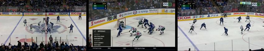
Author’s Declaration

This thesis consists of material all of which I authored or co-authored: see Statement of
Contributions included in this thesis. This is a true copy of the thesis, including any
required final revisions, as accepted by my examiners.

I understand that my thesis may be made electronically available to the public.

                                           ii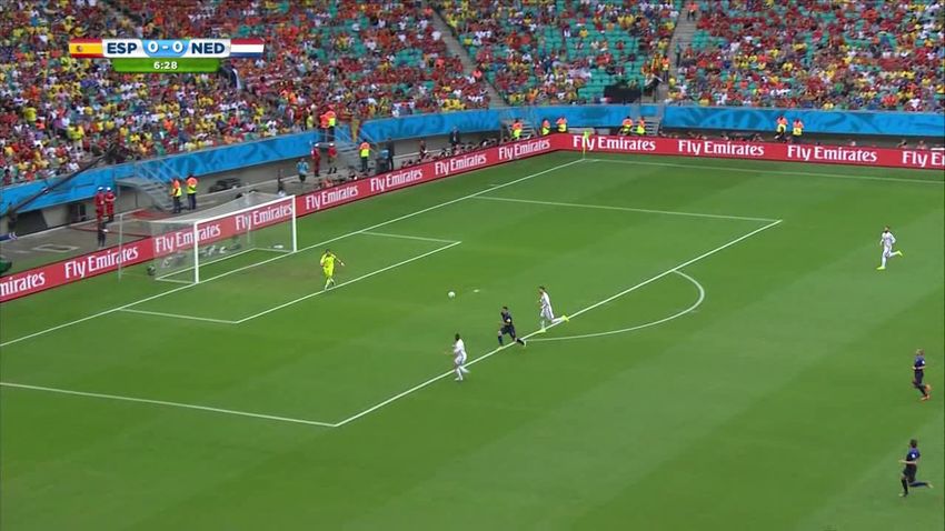
Statement of Contributions

Chapter 3 of this thesis contains content from the previously published paper:

     Pascale Walters, Mehrnaz Fani, David Clausi, and Alexander Wong. 2020. A
     tool for annotating homographies from hockey broadcast video. In Journal of
     Computational Vision and Imaging Systems, Volume 6, Issue 1.

Mehrnaz Fani, David Clausi, and Alexander Wong contributed to the conceptualization
and deployment of this work.

Chapter 4 of this thesis contains content from the previously published paper:

     Pascale Walters, Mehrnaz Fani, David Clausi, and Alexander Wong. 2020.
     BenderNet and RingerNet: Highly efficient line segmentation deep neural net-
     work architectures for ice rink localization. In Journal of Computational Vision
     and Imaging Systems, Volume 6, Issue 1.

Mehrnaz Fani, David Clausi, and Alexander Wong contributed to the conceptualization of
this work. Alexander Wong contributed to the editing of a completed draft of this paper.

                                            iii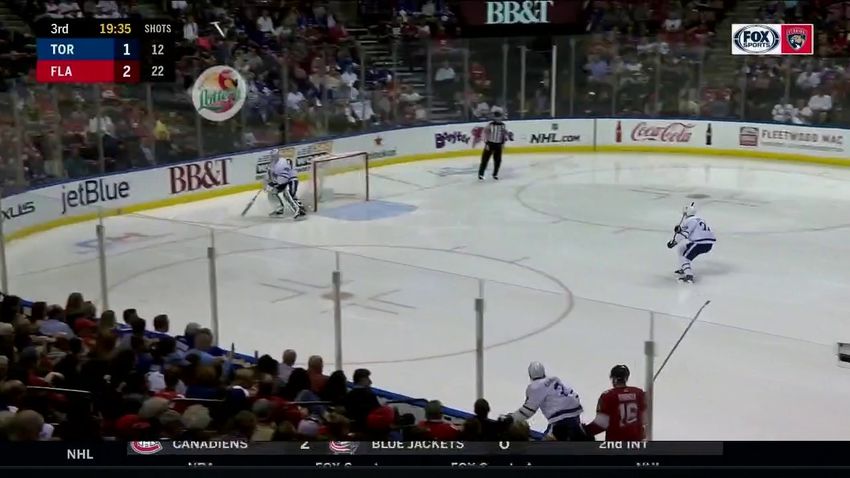
Abstract

    Using computer vision-based technology in ice hockey has recently been embraced as
it allows for the automatic collection of analytics. This data would be too expensive and
time-consuming to otherwise collect manually. The insights gained from these analytics
allow for a more in-depth understanding of the game, which can influence coaching and
management decisions. A fundamental component of automatically deriving analytics from
hockey broadcast video is ice rink localization. In broadcast video of hockey games, the
camera pans, tilts, and zooms to follow the play. To compensate for this motion and get
the absolute locations of the players and puck on the ice, an ice rink localization pipeline
must find the perspective transform that maps each frame to an overhead view of the rink.
    The lack of publicly available datasets makes it difficult to perform research into ice
rink localization. A novel annotation tool and dataset are presented, which includes 7,721
frames from National Hockey League game broadcasts.
   Since ice rink localization is a component of a full hockey analytics pipeline, it is
important that these methods be as efficient as possible to reduce the run time. Small
neural networks that reduce inference time while maintaining high accuracy can be used
as an intermediate step to perform ice rink localization by segmenting the lines from the
playing surface.
    Ice rink localization methods tend to infer the camera calibration of each frame in a
broadcast sequence individually. This results in perturbations in the output of the pipeline,
as there is no consideration of the camera calibrations of the frames before and after in
the sequence. One way to reduce the noise in the output is to add a post-processing step
after the ice has been localized to smooth the camera parameters and closely simulate
the camera’s motion. Several methods for extracting the pan, tilt, and zoom from the
perspective transform matrix are explored. The camera parameters obtained from the
inferred perspective transform can be smoothed to give a visually coherent video output.
Deep neural networks have allowed for the development of architectures that can perform
several tasks at once. A basis for networks that can regress the ice rink localization
parameters and simultaneously smooth them is presented.
    This research provides several approaches for improving ice rink localization methods.
Specifically, the analytics pipelines can become faster and provide better results visually.
This can allow for improved insight into hockey games, which can increase the performance
of the hockey team with reduced cost.

                                             iv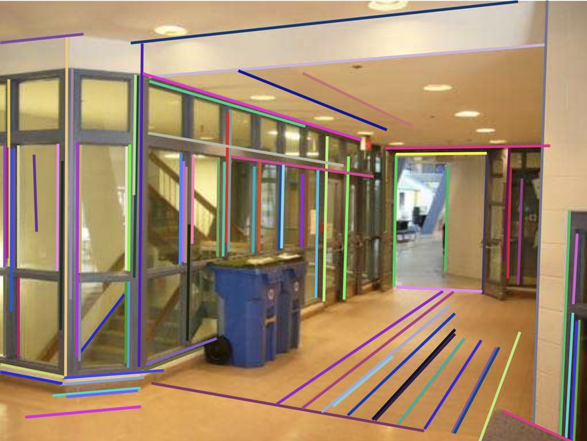
Acknowledgements

   I would like to thank all the people who made this thesis possible.
    Thank you to Prof. David Clausi, Prof. Alex Wong, and Prof. John Zelek for your
support and sharing your knowledge with me. To Mehrnaz Fani and the members of the
Sports Analytics Research Group: thank you for sharing your ideas and helping me when
I got stuck. Thank you to Meghan Chayka and the Stathletes team for believing in a
fledgling female sports analytics researcher.
   This work would not have been possible without my friends and family. To my parents,
Scott and Barbara, and my little sister, Camille. Thank you for all of the love and en-
couragement. Much gratitude to my family away from home: Leigh Anne, Ben, Kathleen,
and Henry. Thank you for taking in this come from away who happened to end up on
the Rock. Finally, a big thank you to my friends who helped me hold it together: Lydia,
Daniel, Ben, Matthew, Dipika, and Rachel.
    Finally, I wish to acknowledge the land on which this thesis was written. Waterloo
is located on the traditional territory of the Neutral, Anishinaabeg, and Haudenosaunee
peoples; Toronto is located on the traditional land of the Huron-Wendat, the Seneca, and
the Mississaugas of the Credit River; and St. John’s is located on the ancestral homelands
of the Beothuk. I am grateful for the opportunity to have lived and worked on these
beautiful lands.

                                            v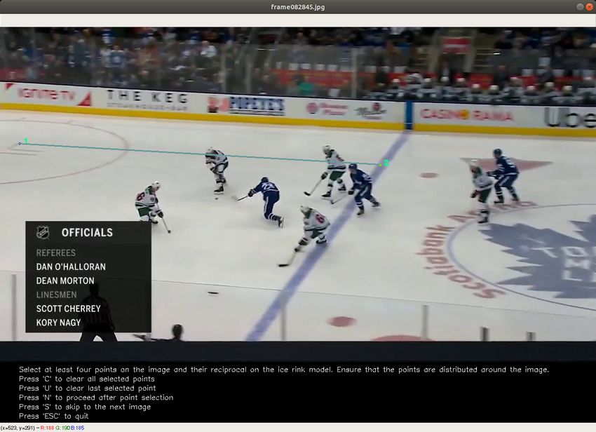
Dedication

To Mommy, Daddy, and Beeble:

 It was the best of times, it was the blurst of times.
                                                   —Charles Montgomery Burns

To Sam:

 Being deeply loved by someone gives you strength, while loving someone deeply
 gives you courage.
                                                                   —Lao Tzu

                                        vi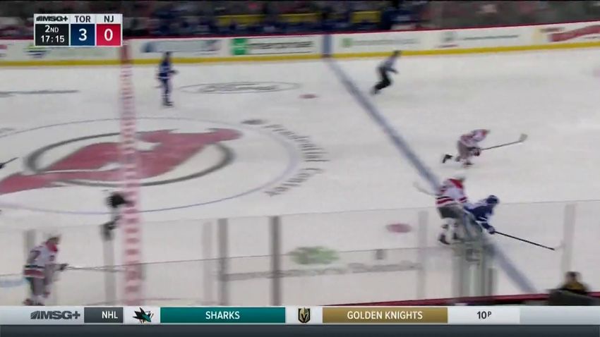
Table of Contents

List of Tables                                                                                 x

List of Figures                                                                                xi

1 Introduction                                                                                 1
   1.1   Motivation . . . . . . . . . . . . . . . . . . . . . . . . . . . . . . . . . . . .     2
   1.2   Thesis Overview . . . . . . . . . . . . . . . . . . . . . . . . . . . . . . . . .      3

2 Background                                                                                   5
   2.1   Computer Vision in Hockey . . . . . . . . . . . . . . . . . . . . . . . . . .          5
   2.2   Sports Field Localization . . . . . . . . . . . . . . . . . . . . . . . . . . . .      7
   2.3   Sports Field Localization Methods . . . . . . . . . . . . . . . . . . . . . . .        8
         2.3.1   Evaluation Metrics . . . . . . . . . . . . . . . . . . . . . . . . . . .      12
   2.4   Sports Field Localization Datasets . . . . . . . . . . . . . . . . . . . . . . .      12
   2.5   General Homography Estimation . . . . . . . . . . . . . . . . . . . . . . .           14
   2.6   Conclusion . . . . . . . . . . . . . . . . . . . . . . . . . . . . . . . . . . . .    16

3 Annotation Tool and Dataset                                                                  17
   3.1   Related Work . . . . . . . . . . . . . . . . . . . . . . . . . . . . . . . . . .      17
   3.2   Motivation . . . . . . . . . . . . . . . . . . . . . . . . . . . . . . . . . . . .    18
   3.3   Annotation Tool     . . . . . . . . . . . . . . . . . . . . . . . . . . . . . . . .   19
   3.4   Description of Dataset . . . . . . . . . . . . . . . . . . . . . . . . . . . . .      21
   3.5   Conclusion . . . . . . . . . . . . . . . . . . . . . . . . . . . . . . . . . . . .    25

                                              vii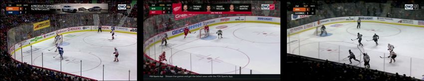
4 Highly Efficient Line Segmentation Deep Neural Network Architectures
  for Ice Rink Localization                                            27
  4.1   Introduction . . . . . . . . . . . . . . . . . . . . . . . . . . . . . . . . . . .   27
  4.2   Related Work . . . . . . . . . . . . . . . . . . . . . . . . . . . . . . . . . .     28
        4.2.1   Line Segmentation for Sports Field Localization . . . . . . . . . . .        28
        4.2.2   Semantic Segmentation . . . . . . . . . . . . . . . . . . . . . . . . .      30
        4.2.3   Line Segment Detection . . . . . . . . . . . . . . . . . . . . . . . .       30
  4.3   Methodology . . . . . . . . . . . . . . . . . . . . . . . . . . . . . . . . . .      31
        4.3.1   Dataset . . . . . . . . . . . . . . . . . . . . . . . . . . . . . . . . .    31
        4.3.2   BenderNet . . . . . . . . . . . . . . . . . . . . . . . . . . . . . . . .    31
        4.3.3   RingerNet . . . . . . . . . . . . . . . . . . . . . . . . . . . . . . . .    33
  4.4   Experimental Setup . . . . . . . . . . . . . . . . . . . . . . . . . . . . . . .     34
        4.4.1   BenderNet . . . . . . . . . . . . . . . . . . . . . . . . . . . . . . . .    34
        4.4.2   RingerNet . . . . . . . . . . . . . . . . . . . . . . . . . . . . . . . .    35
  4.5   Results and Discussion . . . . . . . . . . . . . . . . . . . . . . . . . . . . .     36
  4.6   Conclusion . . . . . . . . . . . . . . . . . . . . . . . . . . . . . . . . . . . .   38

5 Extracting Camera Parameters from Homography Transform Matrix                              39
  5.1   Motivation . . . . . . . . . . . . . . . . . . . . . . . . . . . . . . . . . . . .   39
  5.2   Background . . . . . . . . . . . . . . . . . . . . . . . . . . . . . . . . . . .     40
        5.2.1   Proposed Methods . . . . . . . . . . . . . . . . . . . . . . . . . . .       40
        5.2.2   Camera Parameters in Sports Broadcast Video . . . . . . . . . . . .          41
        5.2.3   Smoothing Homography Based on Camera Parameters . . . . . . .                41
  5.3   Camera Parameter Extraction . . . . . . . . . . . . . . . . . . . . . . . . .        41
        5.3.1   Focal Length . . . . . . . . . . . . . . . . . . . . . . . . . . . . . .     42
        5.3.2   Pan Angle . . . . . . . . . . . . . . . . . . . . . . . . . . . . . . . .    47
        5.3.3   Tilt Angle . . . . . . . . . . . . . . . . . . . . . . . . . . . . . . . .   47
  5.4   Conclusion . . . . . . . . . . . . . . . . . . . . . . . . . . . . . . . . . . . .   51

                                             viii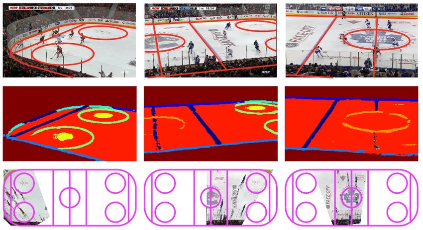
6 Simultaneous Sports Field Localization and Smoothing                                       53
  6.1   Background . . . . . . . . . . . . . . . . . . . . . . . . . . . . . . . . . . .     53
        6.1.1   Deep Networks for Sports Field Localization Refinement . . . . . .           54
        6.1.2   Video Analytics . . . . . . . . . . . . . . . . . . . . . . . . . . . . .    54
  6.2   Experiments . . . . . . . . . . . . . . . . . . . . . . . . . . . . . . . . . . .    55
        6.2.1   Heatmap-Type Architecture . . . . . . . . . . . . . . . . . . . . . .        55
        6.2.2   Long Short-Term Memory Network . . . . . . . . . . . . . . . . . .           58
        6.2.3   Temporal Convolutions . . . . . . . . . . . . . . . . . . . . . . . . .      60
  6.3   Conclusion . . . . . . . . . . . . . . . . . . . . . . . . . . . . . . . . . . . .   62

7 Conclusion                                                                                 63
  7.1   Potential for Future Research . . . . . . . . . . . . . . . . . . . . . . . . .      64
  7.2   Thesis Applicability . . . . . . . . . . . . . . . . . . . . . . . . . . . . . . .   64
  7.3   Thesis Impact . . . . . . . . . . . . . . . . . . . . . . . . . . . . . . . . . .    65

References                                                                                   66

APPENDICES                                                                                   75

A List of Games in Hockey Homography Dataset                                                 76

                                              ix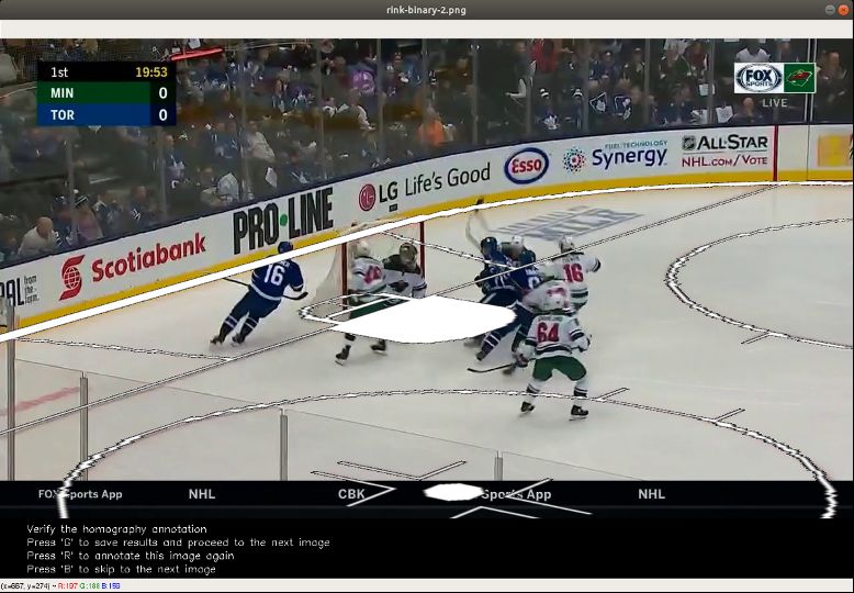
List of Tables

 2.1   Performance of sports field localization methods on the soccer World Cup
       dataset. . . . . . . . . . . . . . . . . . . . . . . . . . . . . . . . . . . . . .   13
 2.2   Datasets for sports field localization. . . . . . . . . . . . . . . . . . . . . .    15

 3.1   Statistics of the data splits from the hockey homography dataset. . . . . .          25

 4.1   Network sizes and performances of three segmentation methods on the NHL
       broadcast video dataset. . . . . . . . . . . . . . . . . . . . . . . . . . . . .     37

 6.1   Performance of the heatmap-type architecture for hockey rink localization.           58
 6.2   Performance of the LSTM network architecture for hockey rink localization.           60
 6.3   Performance of the temporal convolutional network architecture for hockey
       rink localization. . . . . . . . . . . . . . . . . . . . . . . . . . . . . . . . .   62

 A.1 Games in the hockey homography dataset. . . . . . . . . . . . . . . . . . .            76
 A.2 Games in the hockey homography dataset splits. . . . . . . . . . . . . . . .           78

                                             x
List of Figures
1.1 Three broadcast frames from one continuous sequence of play. . . . . . . . 2
1.2 Sports field localization involves determining the transform H from the
hockey broadcast video frame (left) to the overhead view of the rink (right). 3
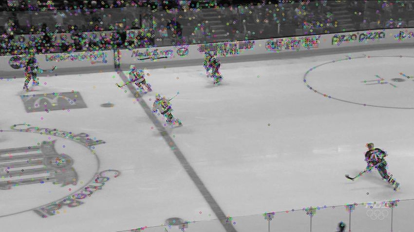
2.1 Three frames showing differences in appearance of the rinks and broadcasts
across the NHL. . . . . . . . . . . . . . . . . . . . . . . . . . . . . . . . . . 8
2.2 SIFT keypoints for a hockey broadcast video frame. . . . . . . . . . . . . . 9
2.3 Line segmentation in the method proposed by Homayounfar et al. . . . . . 10
2.4 Sports field localization pipeline presented by Chen and Little. . . . . . . . 11
2.5 Evaluation metrics for ice rink localization. . . . . . . . . . . . . . . . . . . 13
2.6 Sample output of three sports field localization methods on the soccer World
Cup dataset. . . . . . . . . . . . . . . . . . . . . . . . . . . . . . . . . . . . 14
2.7 Four point parameterization of the homography . . . . . . . . . . . . . . . 16
3.1 Annotation of points on the frame and rink model using the homography
annotation tool. . . . . . . . . . . . . . . . . . . . . . . . . . . . . . . . . . 19
3.2 The best points to annotate with the ice rink localization annotation tool
are at intersections and ends of lines on the ice surface. . . . . . . . . . . . 20
3.3 Homography calculated from the point correspondences is visualized by
warping the frame and rink model. . . . . . . . . . . . . . . . . . . . . . . 21
3.4 Drawing guidelines on the broadcast frame and rink model. . . . . . . . . . 22
3.5 Four sample frames from the hockey homography dataset representing the
diversity in rink appearances between games. . . . . . . . . . . . . . . . . . 23
xi3.6 Distribution of ice surface coverage for all frames in the hockey homography
dataset. . . . . . . . . . . . . . . . . . . . . . . . . . . . . . . . . . . . . . 24
3.7 Failure modes for the hockey homography annotation tool. . . . . . . . . . 26
4.1 Sample hockey and soccer broadcast frames. . . . . . . . . . . . . . . . . . 29
4.2 Line segment detection is a different task than line segmentation in hockey,
as it attempts to find edges of planar surfaces [9]. . . . . . . . . . . . . . . 30
4.3 Three frames from the hockey line segmentation dataset. . . . . . . . . . . 32
4.4 BenderNet architecture. . . . . . . . . . . . . . . . . . . . . . . . . . . . . 32
4.5 Network architecture of RingerNet. . . . . . . . . . . . . . . . . . . . . . . 33
4.6 Typical results for line segmentation with RingerNet and BenderNet. . . . 36
5.1 Focal length calculated with the elements of the homography matrix. . . . 43
5.2 Hockey broadcast frame warped onto the rink model. . . . . . . . . . . . . 43
5.3 Overhead view of a hockey broadcast frame with the focal point. . . . . . . 44
5.4 Distance to focal point and focal length calculated with the elements of the
homography matrix. . . . . . . . . . . . . . . . . . . . . . . . . . . . . . . 45
5.5 Geometry for determining the normalized focal length from the overhead
view of a broadcast frame. . . . . . . . . . . . . . . . . . . . . . . . . . . . 46
5.6 Normalized focal length and distance to focal point. . . . . . . . . . . . . . 48
5.7 Geometry for determining the pan angle φ of the overhead view of the broad-
cast frame. . . . . . . . . . . . . . . . . . . . . . . . . . . . . . . . . . . . . 49
5.8 Calculated pan angle. . . . . . . . . . . . . . . . . . . . . . . . . . . . . . . 50
5.9 Geometry for determining the tilt angle θ of the overhead view of the broad-
cast frame. . . . . . . . . . . . . . . . . . . . . . . . . . . . . . . . . . . . . 51
5.10 Calculated tilt angle. . . . . . . . . . . . . . . . . . . . . . . . . . . . . . . 52
6.1 Locations of the control points on the broadcast frame and warped onto the
rink model according to H. . . . . . . . . . . . . . . . . . . . . . . . . . . . 56
6.2 Architecture of the heatmap-type architecture based on the ResNet-18 ar-
chitecture. . . . . . . . . . . . . . . . . . . . . . . . . . . . . . . . . . . . . 57
xii6.3 Architecture of the multi-scale LSTM architecture for hockey rink localization. 59
6.4 Architecture of the temporal convolutional architecture for hockey rink lo-
calization. . . . . . . . . . . . . . . . . . . . . . . . . . . . . . . . . . . . . 61
xiiiChapter 1
Introduction
Computer vision as a field is an intellectual frontier. Like any frontier, it is
exciting and disorganized, and there is often no reliable authority to appeal
to. Many useful ideas have no theoretical grounding, and some theories are
useless in practice; developed areas are widely scattered, and often one looks
completely inaccessible from the other.
—Forsyth and Ponce, 2002 [29]
Computer vision is currently an impressive field of research. It deals with automating
tasks that would otherwise be done by the human visual system. There is a wide variety
of applications, from medical image analysis to autonomous driving to image retrieval.
Computer vision has automated procedures and obtained state-of-the-art performance.
This field has expanded significantly in the recent years, in part due to the increased
availability and reduction in price of imaging and computation devices, which has spurred
the need for new applications and techniques [29].
A new and exciting application of computer vision is in sports. There is a wide range
of tasks that need to be tackled within this domain, such as player tracking and event
detection [74]. These new insights complement existing systems in sports, such as scouting
reports and player development, by automating manual data collection or generating new
analytics.
One such sport that can benefit from computer vision is ice hockey. In this dissertation,
ice hockey will be the focus of the research and will be referred to by its common name,
hockey.
1Figure 1.1: Three broadcast frames from one continuous sequence of play. The camera
pans, tilts, and zooms to follow the play.
Hockey is a popular sport in Canada, with several professional leagues operating, such
as the NHL (National Hockey League) and CHL (Canadian Hockey League). Furthermore,
Hockey Canada, the national governing body for hockey in Canada, reports that they had
605,963 players and 92,622 coaches registered for the 2019-2020 season [3].
Video analytics of hockey games can be used to provide teams with an advantage over
their competitors, whereby they can gather more data about game events. These data can
be used to influence coaching strategies and management decisions. In addition, the data
can increase fan engagement as sports consumption becomes more digital [81]. The sports
analytics market is rapidly growing and is anticipated to reach revenues of $4.5 billion by
2024 [2].
With many recent developments in the field of computer vision, automatic generation
of sports analysis data from video has become possible. Existing computer vision solutions
analyze video feed from several cameras placed in calibrated locations throughout the arena
[5]. While this technique can be effective, it requires specialized hardware to be deployed at
all arenas where games are played. In situations where this may not be possible, analytics
derived from broadcast footage is an appropriate substitute. Broadcast footage refers to
video that is collected live from at least one camera and distributed for viewing on television
or other platforms.
1.1 Motivation
In hockey, analytics can provide teams with advanced statistics about the individual players
and the team as a whole. These statistics are then used by the teams to influence coaching
decisions, such as assessing player development and preparing to face a certain opponent in
an upcoming game. Management decisions can also be improved, especially when scouting
2Figure 1.2: Sports field localization involves determining the transform H from the hockey
broadcast video frame (left) to the overhead view of the rink (right).
for young players coming up through the minor hockey leagues and other players within
the league looking for a trade.
Collecting these data needed to generate analytics can be resource intensive, especially
if they are manually annotated, making it time-consuming and expensive. This can be
prohibitive for many teams, especially those that may have a lower budget and fewer
employee time resources. Extracting hockey analytics from broadcast video makes them
easier to obtain, which, in turn, makes the sport more equitable for all. This is especially
important as it aligns with the mission of several organizations that aim to increase the
availability of hockey, such as the Hockey Diversity Alliance [4], Black Girl Hockey Club
[1], and the Professional Women’s Hockey Players Association [7].
1.2 Thesis Overview
Analytics from hockey broadcast video are difficult to extract due to the motion of the
broadcast camera. The camera operator pans, tilts, and zooms to follow the play. The
angular subtense is much lower when viewing a hockey broadcast than if the viewer were
there in person. Therefore, the camera operator uses a camera with a long focal length
and captures a small area of the ice at a time [66]. The panning, tilting, and zooming of
the camera allows the viewer to comfortably observe the game. Fig. 1.1 shows three frames
from an NHL broadcast clip where the camera pans, tilts, and zooms to follow the play.
Sports field localization is required to compensate for the motion of the camera to de-
3termine the absolute locations of the players, puck, and referees on the ice surface. Fig. 1.2
shows a frame from a hockey broadcast video and its localization. This is a fundamental
task in extracting analytics from broadcast video, as once the absolute positions are known,
insights about the game can be extracted.
This work attempts to contribute to the research of ice rink localization. A novel
annotation tool for collecting ground truth data from hockey broadcast video and a dataset
for hockey rink localization are presented. Research methods that aim to solve the problem
of hockey broadcast video localization are then discussed. Particularly, this work focuses
on techniques that reduce inference time and improve smoothness of the output. First,
there are two small and fast methods for segmenting lines on the ice surface. Then, two
approaches for smoothing the ice rink localization for a sequence of broadcast video frames
are presented. They are methods for extracting camera parameters, and simultaneous
sports field localization and smoothing using deep networks. The contributions of this
work are new directions of research for improving ice rink localization, which can lead to
improved efficiency for automatic analysis of hockey video.
4Chapter 2
Background
Due to recent significant progress in the field of computer vision and the increased avail-
ability of sports video, there has been much research into automatically extracting sports
analytics from video. This chapter reviews computer vision applications in hockey, sports
field localization, and general homography estimation techniques.
2.1 Computer Vision in Hockey
As part of a pipeline to automatically extract analytics from hockey video, computer vision
techniques have been applied to several tasks. These include:
• Player detection and classification [54, 32],
• Player tracking [55, 82, 65]
• Player identification [16],
• Player pose estimation [61],
• Individual action recognition [14, 27, 80],
• Event detection and classification [78, 76, 55, 75, 25, 82],
• Fight detection [60, 43, 10],
• Broadcast video rectification [33, 18, 51, 13, 83, 40, 26, 63, 77],
5• Puck tracking [66, 79], and
• Logo detection [47].
This list is in a rough order of increasing complexity. When automatically extracting
analytics from hockey, there first needs to be an understanding of where the players are in
each frame (player detection), the team to which they belong (player classification), and
who they are (player re-identification). Next, to gain insight into the game from a sequence
of frames, player tracking is performed to link player detections across a video. This gives
some understanding of how the players move, and it can also be further used to estimate
the pose of each player and recognize what the player is doing, such as skating forwards or
shooting (individual action recognition).
In the sport of hockey, individuals perform actions and events happen at the game
level. For instance, there could be five players skating forwards and three players skating
backwards, but the event would be classified as a zone entry. The event is an action that
may involve multiple players. Beyond classifying the event, it also needs to be associated
with a time (event detection).
Computer vision tasks in hockey require a video source. Many professional hockey
games are broadcast for consumption by viewers who are not physically present at the game.
Using this broadcast footage for computer vision tasks means no additional specialized
hardware is required for generating analytics. Despite broadcast footage being readily
available, it does have some specific challenges. The broadcast camera pans, tilts, and
zooms to follow the play. Compensating for this camera motion is an additional task in
the analytics pipeline.
Some additional areas of research that involve computer vision in hockey are puck
tracking and team logo detection. The puck tracking task can predict the location of the
play by using the absolute location of the puck on the ice as a surrogate [66]. Locating
and identifying team logos and jersey colours can be further used to classify players into
teams.
Recent advances in deep neural networks have shown that using them can achieve
state-of-the-art results in computer vision tasks, including automatic generation of hockey
analytics [79]. Many of the highest performing methods listed in this section use convolu-
tional neural networks (CNNs) or other deep learning architectures [16, 76, 80, 78, 79, 54,
32, 18, 40, 61].
62.2 Sports Field Localization
The sports field localization task involves determining the planar transform between the
view of the hockey rink from the broadcast video frame and an overhead view of a hockey
rink template. This transform is defined by a homography matrix between two views of
the plane of the ice surface (Fig. 1.2).
The homography matrix H is a 3 × 3 matrix with eight degrees of freedom. It relates
the transformation between two planes, up to a scale factor s . Equation 2.1 shows a
T
sample generic homography matrix. It relates the point x0 y 0 1 on the rink model to
T
the point x y 1 on the ice surface in the broadcast frame. The elements of H are a
combination of translation, rotation, and scale [34].
0
x x h11 h12 h13 x
0
s y = H y = h21 h22 h23
y (2.1)
1 1 h31 h32 1 1
This project focuses on broadcast video of NHL games. There are specific challenges
associated with this task. Despite the constant dimensions of the rink in the NHL, there
are varying appearances between rinks in the league, such as graphics on the ice surface
and the boards, illumination, and broadcast camera location. The broadcaster may also
overlay graphics on the video to enhance the viewer experience by adding a score bug, to
display the current score of the game and time in the game, or a news feed. Three frames
in different rinks with different broadcasters are shown in Fig. 2.1.
Over the course of the game, the broadcast features advertisements, player interviews,
and segments with a panel of hockey experts, as well as the game itself. Furthermore,
coverage of the hockey game can feature footage from several cameras set up around the
arena. Hockey rink localization in this dissertation focuses on footage from the main
broadcast camera, which is located in the arena stands above the centre ice line.
The simplest way to calculate the transform between the plane of the ice surface in the
broadcast video and the rink model is to detect field markings, such as points, lines, and
line intersections in the frame then associate them with the corresponding markings in the
model. The homography transform can then be estimated with the direct linear transform
(DLT) algorithm [34]. The DLT algorithm does not give an accurate transform matrix in
the presence of noise in the two sets of image points. A set of inlier point correspondences,
found with the random sample consensus (RANSAC) algorithm, is needed to robustly
estimate the homography transform. In hockey camera calibration, this task is non-trivial:
7Figure 2.1: Three frames showing differences in appearance of the rinks and broadcasts
across the NHL.
the markings are usually small, the field is textureless, and the markings may not be in
the frame or occluded by players [63].
2.3 Sports Field Localization Methods
Playing surface localization is an open research problem in many sports. In sports broad-
casts, the camera pans, tilts, and zooms to follow the play, so that important events fill the
frame [66]. In the literature, there have been several methods described that attempt to
compensate for the camera’s motion. Some of these works also present datasets for sports
field localization.
Early methods tend to use feature detection methods, such as scale-invariant feature
transform (SIFT) [53], speeded up robust features (SURF) [11], and scale-invariant feature
operator (SFOP) [30]. Okuma et al. manually find an initial homography estimate, then
use Kanade-Lucas-Tomasi (KLT) features to find homography transforms between frames
in broadcast hockey video [65]. Hayet et al. perform soccer field localization using colour-
based line detection and KLT features [36]. Hess and Fern use the Harris affine region
detector and SIFT features for registering broadcast football footage [38]. Hayet and
Piater use colour-based line tracking, as well as KLT and Harris features for broadcast
soccer video [35]. Gupta et al. use SFOP and SIFT features for broadcast hockey video
[33]. Wen et al. use SURF features and colour-based playing field extraction for basketball
[84]. Zeng et al. use a similar strategy for field hockey video [87].
These early methods tend to only perform under controlled conditions and don’t trans-
late well to sports or situations for which they weren’t originally developed. This means
that changes in factors such lighting, player appearance, and playing surface appearance
could cause these techniques to fail.
8Figure 2.2: SIFT keypoints (coloured circles) for a hockey broadcast video frame. Most of
the keypoints are detected on the stands and players, rather than the ice surface.
SIFT keypoints for a hockey broadcast frame are shown in Fig. 2.2. Most of the
keypoints are on the players and the spectators in the stands, rather than on the ice
surface.
The most common method for sports field localization uses line detection and matching.
Some methods described in the previous paragraph use both feature detection and line
detection [35, 33]. Thomas uses the Hough transform to extract lines from soccer video
and matches them to a field template with a least squares algorithm [73]. Kim and Hong
use the Hough transform to detect lines on the playing surface of soccer video and camera
parameter-guided line tracking to estimate the camera parameters [46]. Carr et al. align
the lines visible in field hockey video to a field template with gradient-based optimization
[15]. Dubrofsky and Woodham use both point and line correspondences for estimating
the homography with a hockey dataset [26]. Yao et al. also detect lines on a soccer field
with the Hough transform and determine point correspondences with a field template by
parameterizing the nature of four line crossings in the frame [86].
Homayounfar et al. detect lines with a VGG16 semantic segmentation network, use
them to minimize the energy of the vanishing point, and estimate the camera position via
9Figure 2.3: Line segmentation in the method proposed by Homayounfar et al. [40]. The
results of their line segmentation with a VGG16 network are in the middle row.
branch and bound [40]. They perform their work on the World Cup soccer dataset and
the SportLogiq hockey dataset. The output of their line segmentation method and sports
field localization are shown in Fig. 2.3.
Sharma et al. and Chen and Little use the pix2pix network to extract the lines from
the playing surface on a dataset of soccer broadcast video. Both works then compare the
extracted edge images to a database of synthetic edge images with known homographies
in order to localize the playing field [17, 69]. Skinner and Zollman performed playing field
localization for rugby games filmed with a smartphone camera from the stands. They
extract lines with the Hough transform and match the vertical lines to a template of the
pitch [71]. Cuevas et al. detect the lines on a soccer field and classify them to match
them to a template of the field [22]. Tsurusaki et al. use the line segment detector to
find intersections of lines on a soccer field, then match them to a template of a standard
soccer field using an intersection refinement algorithm [77]. These methods tend to work
relatively well, however they struggle in sports where the players are large compared to the
playing surface, as in hockey. They also tend to fail when the video frame does not have
many lines in it.
Another category of sports field localization techniques extract zones from the playing
surface, rather than the lines, as this may be more robust [68]. Zeng et al. extract the
zones and use feature detection in their method [87]. Sha et al. detect the zones from
10Figure 2.4: Sports field localization pipeline presented by Chen and Little [17]. They
generate a feature-pose database to match the input broadcast video frame to a frame
with known homography matrix.
soccer and basketball datasets. They initialize the camera pose estimation through a
dictionary lookup and refine the pose with a spatial transformer network [68]. Tarashima
performs semantic segmentation of the zones as part of a multi-task learning approach for
a basketball dataset [72].
Furthermore, there are sports field localization methods that do not necessarily fall into
the previously discussed categories. As discussed in the previous two paragraphs, there are
some methods that use a dictionary search step in their sports field localization pipeline
[69, 17, 71, 22, 68]. The architecture of Chen and Little’s sports field localization pipeline
that uses a feature-pose database to match the segmented lines from the input broadcast
video frame to a frame with known homography matrix. The dictionary search methods
require a large training set that represents all the test data the method will see. The
database of frames can also become quite large, increasing the inference time.
Ghanem et al. perform image patch matching in a football dataset [31]. Citraro et
al. segment keypoints based on intersections of the lines on the playing surface and match
them to a template for basketball, volleyball, and soccer datasets [21]. Similarly, Nie et al.
segment a uniform grid of points on the playing surface and compute dense features for
localizing video of soccer, football, hockey, basketball, and tennis [63]. Jiang et al. propose
a method for soccer and hockey video to refine homography estimates by concatenating
the warped template and frame, then minimizing estimation error [45].
11The wide variety of methods that have been described in the literature shows that there
is no one method that works particularly well for all sports applications. Furthermore, these
methods do not tend to publicly release their code and dataset. It is therefore incredibly
difficult to assess the accuracy and inference time for our project requirements. Recently
described techniques show that deep network architectures achieve better performance with
faster computation [45, 72, 21, 17].
Further research is needed into a method for hockey rink localization that can be
evaluated on a novel dataset of NHL broadcast video, described in Chapter 3. Most of the
sports field localization methods that are presented in the literature do not report their
methods on hockey broadcast video, with the exception of Homayounfar et al. [40], Jiang
et al. [45], and Nie et al. [63]. A new method is needed that overcomes the shortcomings
of these methods, namely a short inference time, high accuracy, and temporal constancy
over a video sequence of hockey broadcast frames.
2.3.1 Evaluation Metrics
Sports field localization methods tend to use either IOUpart or IOUwhole or both. These
two metrics rely on comparing the ground truth transform to the inferred transform.
IOUpart is the intersection over union of the frame warped onto the rink according to
the ground truth and predicted homographies. In Fig. 2.5a, the yellow shape represents
the ground truth broadcast frame warp and the shape outlined in orange is the predicted
broadcast frame warp. The IOUpart would be the intersection over union of these two
shapes.
IOUwhole is the intersection over union of the whole rink warped according to the pre-
dicted sports field localization transform. In Fig. 2.5b, IOUwhole is the intersection over
union of the ground truth (red rink shape) and the predicted rink (yellow outline).
It is recommended to only use the IOUwhole score of a method because it considers the
whole playing surface, rather than just the part of the field visible in the broadcast frame
[21]. In the worst case scenario, the IOUpart could be perfect while the IOUwhole is much
lower, due to it considering the performance of the method on the whole field.
2.4 Sports Field Localization Datasets
Research within the area of sports field localization can be difficult due to the lack of pub-
licly available datasets and the variety of test datasets on which methods in the literature
12(a) IOUpart (b) IOUwhole
Figure 2.5: Evaluation metrics for ice rink localization.
IOUpart IOUwhole Inference Time (s)
Homayounfar et al. [40] 83.0 0.44
Sharma et al. [69] 91.4 0.21
Chen and Little [17] 94.5 89.4 0.5
Sha et al. [68] 93.2 88.3 0.004
Citraro et al. [21] 93.9 0.125
Jiang et al. [45] 95.1 89.8 1.36
Nie et al. [63] 95.9 91.6 0.5
Tsurusaki et al.2 [77] 97.4
Table 2.1: Performance of sports field localization methods on the soccer World Cup
dataset. Numbers in bold are the best performance for each metric.
are evaluated. To our knowledge, the only publicly available dataset is the soccer World
Cup dataset1 . The dataset contains broadcast video from 20 soccer games, and has 209
training frames and 186 testing frames [40]. There are eight papers that have reported
the performance of their methods on this dataset [40, 69, 17, 68, 21, 45, 63, 77]. The
performance of these methods are reported in Table 2.1.
Sample output of three of the sports field localization methods on the soccer World
Cup dataset is shown in Fig. 2.6. The method proposed by Sha et al. achieves the lowest
inference time. Despite including a dictionary search step for camera pose initialization,
which could potentially slow the method, they are able to reduce the search space and use
an end-to-end architecture [68]. The authors report that their method struggles with the
1
http://www.cs.toronto.edu/~namdar/data/soccer_data.tar.gz
2
The performance of the method proposed by Tsurusaki et al. is only reported on the 18 best performing
frames in the test dataset.
13Figure 2.6: Sample output of three sports field localization methods on the soccer World
Cup dataset. From left to right: Homayounfar et al. [40], Chen and Little [17], Nie et al.
[63].
semantic segmentation component of their architecture, due to insufficient training data,
which gives lower IOUpart and IOUwhole scores. Citraro et al. achieves the best IOUwhole
score, which, they argue, is the only accuracy metric that is significant [21]. Their sports
field localization pipeline is unique in that it considers the locations of the players on the
field, which requires them to augment the World Cup dataset by manually annotating the
player positions. When this component is removed, the IOUwhole drops to 90.5, which is
lower than most of the other methods. Nie et al. achieve the highest IOUpart score using
their dense features approach, however their IOUwhole is still lower than Citraro et al. [63].
Other datasets that have been described for sports field localization but may or may
not be available publicly are listed in Table 2.2.
2.5 General Homography Estimation
Sports field localization is a special case of homography estimation, where the structure of
the playing field plane is known [63]. There are two main approaches for estimating the
homography transform between two views of a plane: keypoint detection and parameter
regression.
Keypoint detection involves finding salient points on the two views and their correspon-
dences. Some techniques include using descriptors such as SIFT [53], SURF [11], and SFOP
[30]. Once corresponding keypoints are found, the algorithm with RANSAC is used to get
an estimate of the homography [34]. Deep learning techniques can also be used to detect
keypoints in situations without uniform appearance and dynamic scenes [63]. For example,
human pose estimation has had success with deep network architectures [50, 20, 56].
Traditional image processing techniques for homography estimation that use hand-
crafted features, such as corner and edge detection, tend to face certain downfalls. First,
14Dataset Number of Images Publicly Available?
World Cup Soccer [69] 500 7
World Cup Soccer [40] 209 (train), 186 (test) 3
Hockey [40, 45] 1.67M 7
Basketball [21] 50,127 ?
Volleyball [21] 12,987 ?
MLS Soccer [21] 14,160 7
Basketball [72] 1,232 7
College Basketball [68] 526 (train), 114 (test) 7
SportsFields [63] 1,833 (train), 1,134 (test) 7
Table 2.2: Datasets for sports field localization. Datasets that have a ? in the Publicly
Available column were reported in their respective papers as being made available, but do
not seem to actually be so.
these feature detectors are sensitive to large variation in appearance and scenes that are
not static. Deep networks use learned features, which capture context from a larger area
of the image, as compared to the handcrafted feature detectors. Deep networks are more
robust to local changes in appearance.
Deep network architectures have also made it possible to directly estimate the param-
eters of the homography transform between two frames [24, 62, 48]. DeTone were the first
to do this task, and they parameterized the homography matrix as the mapping of four
corners from one image to the next image in a randomly selected rectangle. They use a
10-layer network on the MS-COCO dataset, which is tested by randomly perturbing the
corners of the images [24]. The four point parameterization is shown in Fig. 2.7. Nguyen
et al. propose a method for stitching together aerial images. They use an unsupervised
approach that extends the work of DeTone et al. by adding a spatial transform layer and
a photometric loss. These two methods work well for image pairs that can be fully aligned
with a homography transform [62]. Le et al. attempt to solve the problem for dynamic
scenes (i.e., those where there is motion in the foreground and background). They train
a deep neural network for multi-task learning that performs both homography estimation
and dynamic content detection [48].
15Figure 2.7: Four point parameterization of the homography [24]. Hmatrix is the 3 × 3
homography matrix that represents the perspective transform between the two squares.
H4point is the 4-point parameterization of the homography. It represents the change in the
coordinates of the corners of a randomly selected rectangle from the first image.
2.6 Conclusion
This chapter extensively explores work in the literature for computer vision applications
in hockey, sports field localization, and general homography estimation methods. There is
a lack of publicly available datasets on which to perform research for ice rink localization
for hockey broadcast video. The many approaches that have been published show that
no consensus has been reached for the optimal way to solve the problem of sports field
localization. Each new contribution to this field proposes a completely new method, rather
than attempting to incrementally improve the methods that already exists. Some areas
in which these proposed approaches can be enhanced are in reducing inference time and
improving visual coherence in the output.
16Chapter 3
Annotation Tool and Dataset
Many techniques have been described in the literature to perform sports camera calibration
with deep learning methods [40, 69, 17, 72, 45, 21, 68]. However, the authors of these
methods do not release the datasets that they have used for training and testing, with the
exception of the World Cup dataset for soccer games [40]. Therefore, a novel dataset is
required in order to develop new ice rink localization techniques.
In this chapter, a new annotation tool for collecting homographies from frames of hockey
broadcast videos is presented. It relies on annotating corresponding points on each frame
and a model of the overhead view of the ice surface. With this tool, we have collected a
dataset of frames, each of which has a corresponding homography and time in its video
sequence.
3.1 Related Work
In the literature, each method for performing sports field localization tends to come with
its own sports field localization dataset. These datasets, with the exception of the World
Cup dataset [40], have not publicly been made available.
Several sports have been the focus of field localization techniques. Datasets described in
the literature include volleyball [21], basketball [72], and hockey [45]. Table 2.2 compares
the datasets used for sports field localization methods.
The only publicly available dataset for this problem, World Cup Soccer, has 395 an-
notated frames. Each frame has an associated homography, but no temporal information
(i.e., the frames have been randomly collected from broadcast footage) [68].
17All methods report that their datasets have been annotated with point correspondences,
and the associated homography determined with the DLT algorithm. To our knowledge,
no annotation tool for sports field localization has been released.
Tarashima describes an annotation method for their basketball dataset, whereby only
pre-specified intersections of lines on the playing surface and corresponding points on over-
head playing surface model are annotated [72]. Citraro et al. describe a semi-automated
method that was used for their datasets [21]. The annotation tool automatically tracks
keypoints and the user provides corrections as needed.
3.2 Motivation
This research is the result of a partnership between Stathletes, a Canadian hockey analytics
company, and the Sports Analytics Research Group, within the Vision and Image Process-
ing Lab at the University of Waterloo. Stathletes analysts manually annotate broadcast
footage of hockey games to collect analytics that they then distribute to teams and leagues.
Their analysts are very skilled and quick at annotation tasks, such as rapidly and accu-
rately clicking on an image with a mouse, and this annotation tool was developed with
their expertise in mind.
There were several design constraints that were faced when developing this annota-
tion tool. The Stathletes analysts are not necessarily familiar with coding and using the
command-line interface of a computer. This meant that the tool needed to be portable,
and not provided to them as a series of code files and dependencies that needed to be
installed on their computers. The tool needed to be shared as a single file that contained
all code dependencies is opened and run on the user’s computer by double-clicking on an
icon, similar to other standard Windows applications.
These analysts also work on computers running the Microsoft Windows operating sys-
tem, rather than the computer on which this code was developed, which runs the Ubuntu
operating system. Finally, we only had one graduate student to develop this application.
This meant that the tool could not have too many features, which would take too long to
develop.
The challenge with this application was striking a balance between having a tool that
the Stathletes analysts could use efficiently and not having so many features that the re-
search team was spending too much time on development, rather than performing research.
18(a) Points annotated on a frame from (b) Corresponding points annotated on the over-
a hockey broadcast video. head model of an NHL rink.
Figure 3.1: Annotation of points on the frame and rink model using the homography
annotation tool.
3.3 Annotation Tool
Obtaining the true homography matrix for each frame in a broadcast video sequence proved
to be impossible, as there is no way to obtain the camera parameters from the broadcast.
For this reason, we needed to collect our own annotated dataset.
The annotation tool works by having the operator select point correspondences be-
tween frames in NHL broadcast footage and a standard model of the rink surface. Point
correspondences were selected as the means for collecting the ground truth homography
matrices because it was easily implemented in Python with OpenCV’s findHomography
method [6]. This function uses the DLT algorithm with RANSAC to determine the best
homography matrix between the corresponding 2D point annotations.
The tool was developed in Python and released as an executable using the PyInstaller
library for use by analysts at Stathletes [8]. To use the tool, the user selects corresponding
points, alternating between the frame and the rink model (Fig. 3.1). The points are
numbered and coloured to match on the frame and rink template.
Users are instructed to select as many points as possible. The best points (i.e., highest
precision) are located at the intersections and ends of lines on the playing surface. For
example, the intersection of the goal line and boards, the intersection of the hash marks
and faceoff circle, and the base of the goal post. The users are also able to zoom in and
out to ensure that they are clicking on the correct position.
After the user has selected at least four corresponding points, representing the eight
19Figure 3.2: The best points to annotate with the ice rink localization annotation tool are
at intersections and ends of lines on the ice surface (pink dots).
degrees of freedom in the homography matrix, the tool then calculates and displays the
results of that homography warping. The frame is warped and overlayed on top of the rink
model and the rink model is warped on top of the frame (Fig. 3.3).
The homography is determined with DLT and RANSAC for outlier rejection. We have
tuned the RANSAC parameters for the highest visual accuracy, while requiring the fewest
point annotations.
The user can then accept, reject, or edit their annotations after viewing the result of
their annotations. The average time to annotate each frame is 90 seconds. The commands
are represented with keyboard shortcuts and annotations are stored as clicks. This closely
resembles the annotation workflow with which the Stathletes analysts are familiar.
The output is stored in JSON format, which is sent back to the University of Waterloo
team once the annotations are complete. Upon receiving the output, the annotations are
further verified by the researchers.
While Stathletes analysts have been using the annotation application, they have pro-
vided feedback and suggestions to the University of Waterloo developers. These suggestions
have allowed for the annotations to be more accurate and the analysts to process more
frames faster. For example, we added keyboard shortcuts to allow for the user to quickly
delete pairs of annotations that add noise to the homography estimate. When the user re-
views their annotation and chooses to redo the selected points, rather then having to start
20(a) The warped frame overlayed on the (b) The warped rink model overlayed on the
rink model. frame.
Figure 3.3: During the verification stage of the homography annotation tool, the homog-
raphy calculated from the point correspondences is visualized by warping the frame and
rink model.
the annotation from the beginning, they are able to alter the points they have already
selected.
While the broadcast frames were being annotated, there were certain frames that were
the most difficult annotate well. These were the frames that were mostly filled by the area
of the ice around either blue line. The lack of high fidelity keypoints made it difficult to
obtain an accurate and robust annotation. A feature was added to allow the users to draw
guidelines in order to obtain accurate annotations in areas of open ice (Fig. 3.4).
3.4 Description of Dataset
The hockey homography dataset collected with the annotation tool has 7,721 annotated
frames from 24 separate game broadcasts from the 2018-19 NHL season. Two to three
shots, or sequences of dynamic game play, were extracted from each game, each lasting
approximately 30 seconds, for a total of 84 shots. All sequences were captured by the main
broadcast camera, which is located in the stands above the centre line of the ice surface.
The videos were sampled at 1.5 frames per second (fps). The frames come from several
different broadcasters, which means that the overlayed graphics are not the same across
the dataset. A variety of home teams also means that there are different designs (e.g.,
team logo) embedded in the ice. Fig. 3.5 shows four sample frames from the dataset.
21(a) Guideline drawn on the broadcast (b) Guideline drawn on the rink model.
frame.
Figure 3.4: Drawing guidelines on the broadcast frame and rink model. This allows the
used to get a high fidelity annotation in an area with few keypoints. In this pair of frame
and rink model, a guideline (turquoise) is drawn from the faceoff circle line (1) straight
out to the blue line. A keypoint (2) can now be precisely annotated on the blue line where
there would otherwise be no line intersections or endings.
In hockey broadcasts, the camera pans, tilts, and zooms to attempt to fill each frame
with the play. This means that a significant portion of the ice surface is not shown in
each frame [44]. However, when the whole dataset is aggregated, we obtain 100% coverage
of the whole ice surface. Individually, the mean coverage of a frame is 24.1% of the ice
surface. A histogram of the ice surface coverage for all frames is shown in Fig. 3.6.
The dataset is divided into train, test, and validation splits for research on ice rink
localization methods randomly according to the games and venues from which the frames
come. This ensures that the methods that memorize a rink appearance will obtain poor
validation and test scores. Table 3.1 shows statistics about the splits of the dataset. Further
details are shown in Appendix A.
Our dataset is to be used for training and testing methods for ice rink localization of
NHL games. In the NHL there is a fixed set of venues, where every game is played in
the home rink of one of the 31 teams. There are some exceptions to this rule, such as
the NHL Winter Classic, where a game is played in an outdoor venue. However, we can
assume that our methods only need to be used for use in the indoor rinks. An ideal dataset
would therefore have games played in each of the 31 possible rinks. We could train and
evaluate our methods on this dataset, since we would never be faced with an unknown
rink. Another approach would be to train separate models with the same architecture for
each of the rinks. In this way, there would be one model for each rink that works perfectly,
22Figure 3.5: Four sample frames from the hockey homography dataset representing the
diversity in rink appearances between games.
23Figure 3.6: Distribution of ice surface coverage for all frames in the hockey homography
dataset.
24Split Number of Games Number of Frames
Train 21 6,524
Validation 2 706
Test 1 491
Total 24 7,721
Table 3.1: Statistics of the data splits from the hockey homography dataset.
rather than having to have a method that can generalize to all rinks in the league. Due to
the difficulty of collecting annotations, our dataset contains games that were played in 13
rinks across the league.
During the annotation process, 450 frames were rejected due to the inability to get
a satisfactory annotation. These frames are not included in the dataset descriptions in
Tables 3.1 or A.1. Some failure modes for these frames included blur due to camera
motion, occlusion by broadcast graphics, and too few high fidelity keypoints (Fig. 3.7).
3.5 Conclusion
We have developed a homography annotation tool to collect the transforms between frames
from hockey broadcast video to an overhead rink model. The tool determines the ground
truth transform through at least four point correspondences of landmarks on the ice. We
also have collected a dataset of 7,721 hockey broadcast homographies. The dataset fills
the gap of no publicly available ice rink localization datasets for research into broadcast
camera calibration methods.
25Figure 3.7: Failure modes for the hockey homography annotation tool. Clockwise from top
left: ice blocked by broadcast graphic; too zoomed in, not enough high fidelity keypoints;
motion blur; area around blue line, too few high fidelity keypoints.
26Chapter 4
Highly Efficient Line Segmentation
Deep Neural Network Architectures
for Ice Rink Localization
Hockey analytics generated in real-time can be used by coaches and players to adapt their
play to their opponents. It also allows for live data to be generated for sports betting and
increased immersion for the fans in the game.
Inference from ice rink localization methods that rely on deep neural networks can be
accelerated by making the network smaller. This means reducing the number of operations
during inference. This chapter discusses two methods that use deep neural networks with a
reduced number of parameters to segment the lines from the ice surface as an intermediate
step for ice rink localization.
4.1 Introduction
Sports field localization is required to determine the absolute positions of the players and
the puck on the ice, regardless of the broadcast camera’s position. There have been methods
developed to perform this analysis [17, 40, 45, 69], and several of these methods require
segmentation of the lines on the playing field as an intermediate step. The resulting
edge maps are used for further processing, such as for vanishing point estimation [40] or
dictionary lookup [17, 69].
27Despite the relative successes of these methods, there seems to be little focus into the
selection of the semantic segmentation methods and justification for their use, but more
into the downstream analysis [17, 40, 69]. This work deals solely with the line segmentation
problem from hockey broadcast video, and proposes two efficient deep networks to solve it.
This work details two methods for approaching real-time performance for line segmen-
tation from hockey broadcast video. BenderNet and RingerNet are small networks that
achieve high accuracy on our annotated dataset from NHL games.
The contributions of this work are two lightweight semantic segmentation networks that
effectively detect the lines on the playing surface from hockey broadcast video. BenderNet
is two conditional generative adversarial networks (GANs) and RingerNet is segmentation
network that uses dilated depthwise separable convolutions.
BenderNet achieves a mean intersection over union (mIOU) score of 31.12 with 2.8
million parameters and RingerNet achieves an mIOU score of 55.69 with 0.78 million
parameters on the test split of the labelled dataset used in this work [52]. This opens the
door for further research into small networks for line segmentation as an intermediate step
for homography estimation.
4.2 Related Work
Works related to small semantic segmentation networks and sports field localization are
reviewed here.
4.2.1 Line Segmentation for Sports Field Localization
In the literature, there have been several papers that attempt to solve the problem of sports
field localization. Of these published methods, there are some that require segmenting the
lines and outline of the ice surface as an intermediate step [17, 40, 69]. To our knowledge,
there have not been any published methods that intensively explore the line segmentation
component.
The sports field localization methods in the literature have some shortcomings, however,
such as methods that only report performance on frames from soccer broadcast video
[17, 69] and a lack of availability of the source code [69].
Line segmentation from broadcast soccer games differs from the same task with hockey
for several reasons. First, the players are much smaller in relation to the field markings in
28You can also read