Classification of Urban Morphology with Deep Learning: Application on Urban Vitality - arXiv
←
→
Page content transcription
If your browser does not render page correctly, please read the page content below
Classification of Urban Morphology with Deep Learning:
                                                             Application on Urban Vitality

                                                          Wangyang Chena , Abraham Noah Wua , Filip Biljeckia,b,∗
                                                        a Department    of Architecture, National University of Singapore, Singapore
                                                        b Department    of Real Estate, National University of Singapore, Singapore
arXiv:2105.09908v2 [cs.CV] 8 Jul 2021

                                        Abstract
                                            There is a prevailing trend to study urban morphology quantitatively thanks to the
                                        growing accessibility to various forms of spatial big data, increasing computing power,
                                        and use cases benefiting from such information. The methods developed up to now
                                        measure urban morphology with numerical indices describing density, proportion, and
                                        mixture, but they do not directly represent morphological features from the human’s vi-
                                        sual and intuitive perspective. We take the first step to bridge the gap by proposing a deep
                                        learning-based technique to automatically classify road networks into four classes on a
                                        visual basis. The method is implemented by generating an image of the street network
                                        (Colored Road Hierarchy Diagram), which we introduce in this paper, and classifying it
                                        using a deep convolutional neural network (ResNet-34). The model achieves an overall
                                        classification accuracy of 0.875. Nine cities around the world are selected as the study
                                        areas with their road networks acquired from OpenStreetMap. Latent subgroups among
                                        the cities are uncovered through clustering on the percentage of each road network cate-
                                        gory. In the subsequent part of the paper, we focus on the usability of such classification:
                                        we apply our method in a case study of urban vitality prediction. An advanced tree-based
                                        regression model (LightGBM) is for the first time designated to establish the relation-
                                        ship between morphological indices and vitality indicators. The effect of road network
                                        classification is found to be small but positively associated with urban vitality. This
                                        work expands the toolkit of quantitative urban morphology study with new techniques,
                                        supporting further studies in the future.
                                        Keywords: Urban form, Computer vision, GIScience, Urban vibrancy, Street network,
                                        Urban analytics

                                           ∗ Corresponding
                                                         author
                                           Email addresses: e0403826@u.nus.edu (Wangyang Chen), abraham@nus.edu.sg (Abraham Noah
                                        Wu), filip@nus.edu.sg (Filip Biljecki)

                                        Preprint submitted to journal                                                                  July 9, 2021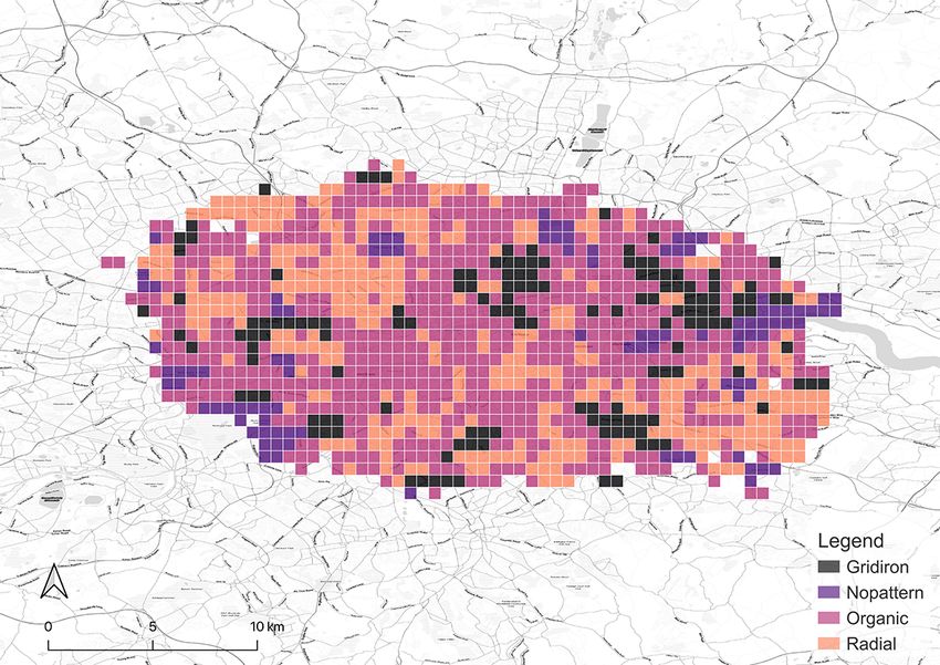
1. Introduction
     Urban morphology is the study of the formation of human settlements and the pro-
cess of their formation and transformation (Moudon, 1997). It dissects the urban built
environment into components (building, street, block, etc.) and aims to understand the
running pattern among each component, the interaction between components, and influ-
ence on a multitude of phenomena such as urban microclimate and energy (Yuan et al.,
2019; Garbasevschi et al., 2021).
     The mainstream of quantitative morphological study operates by transforming urban
entities into numerical indices. There exists a wealth of literature concentrating on the
quantification of the characters of building and space. Lynch (1984) quantitatively stud-
ies the relationship among floor space, distribution of open space, building height, and
other elements. Alexander (1977) lists and explains the indicators of urban morphology
at the city, neighborhood, and building levels but has not provided the corresponding cal-
culation methods. Berghauser Pont and Haupt (2007) propose a graph-based approach
to analyze the urban form on the ground of four major morphological indicators and
denominated this method as “spatial matrix” (Berghauser-Pont and Haupt, 2010). Other
scholars take road networks as the point of departure. Network-based methods repre-
sented by spatial syntax are put forward to analyze the configuration of networks (Hillier
and Hanson, 1984;1989;1988;; Hillier, 1996). The analytical techniques of space syntax
have been utilized in various studies related to urban morphology (Jiang and Claramunt,
2002; Baran et al., 2008; Ye and Van Nes, 2014). Further, many studies attempt to set up
their morphological index system (Bocher et al., 2018; Li et al., 2020a,b), especially the
recent study of Martino et al. (2021), which includes nearly every measurement men-
tioned above. While these methods have contributed to explaining urban morphology in
a more scientific and mathematical manner, they usually rely on calculations on vector
spatial data.
     The advent of new techniques such as deep learning, which are gaining momentum
in urban studies (Wu and Biljecki, 2021; Zhang and Cheng, 2020; Ding et al., 2021), may
enable more innovative ways to measure urban morphology. In this paper, we posit that
these techniques are still underexplored in the domain of characterizing the urban form.
Therefore, we aim to develop an approach to extract features from morphological images
with convolutional neural networks, demonstrating the usability of new technologies
such as deep learning in the perennial topic of urban morphology.
     As a case study, we focus on urban vitality, which has been a prevalent topic for
decades. The work of Jacobs (1961) conceptualizes urban vitality as the capacity of the
living environment to motivate the interactions among people and between people and
the environment. We adopt this definition in this paper. The newly available open spatial
big data sources (as opposed to traditional data collected from surveys) provide a great
convenience for the study of urban vitality in the urban area, continuously maintaining it
topical. In fact, many instances of research related to the measurement of urban vitality
have been conducted based on different kinds of data sources.
                                             2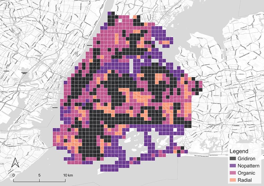
There are two major approaches to assess the intensity of urban vitality, from the
perspective of the built environment and people, respectively. One is by measuring the
capacity of the built environment to boost activities (Lopes and Camanho, 2013; Delclòs-
Alió and Miralles-Guasch, 2018; Yue et al., 2019; Jin et al., 2017; Ye et al., 2018; Zeng
et al., 2018), while the other one is by measuring the density of people (Kim, 2020; Chen
et al., 2019; Wu et al., 2018; Yang et al., 2021; Meng and Xing, 2019; Yue et al., 2017;
Li et al., 2020a). Meanwhile, researchers also adopted a hybrid method to carry out their
assessment (Xia et al., 2020; He et al., 2018; Botta and Gutiérrez-Roig, 2021). Accord-
ing to the definition, urban vitality relates to two aspects, human and environment. As
we cannot guarantee that an individual data source reflects each aspect sufficiently well,
we need to involve multiple data sources for each of them.
     Many previous studies have been devoted to delineating the relationship between
urban morphology and vitality. Regarding the model to establish the relationship, Or-
dinary Least Squares (OLS) regression is the most widespread model, as researchers
have preferred its simplicity and interpretability (Sung and Lee, 2015; Ye et al., 2018;
Yue et al., 2017; Meng and Xing, 2019; Wu et al., 2018; Zarin et al., 2015). However,
the drawback of OLS is also obvious. On the one hand, OLS regression was noted to
disregard the spatial dependence among the places which is deemed commonly existing
(Xia et al., 2020; Li et al., 2020a). On the other hand, the linearity hypothesis on the
relationship between urban morphology and urban vitality was challenged (Yang et al.,
2021). To alleviate the problem, it might be worthwhile to apply a more advanced model
to describe the relationship.
     In this study, tackling the research opportunities and shortcomings described so far,
we mainly aim to fill the following gaps and present the following contributions to the
field: (1) we introduce a supervised deep learning method to classify road networks from
human perception, with the outlook of supporting a wide range of applications in urban
morphology studies; (2) we adopt the method in a case study of urban vitality predic-
tion and investigate its effectiveness; (3) we propose additional dimensions to indicate
urban vitality and mitigate biases caused by single indicator, alleviating one of the key
shortcomings of related work; and (4) we adopt a more advanced model to delineate the
relationship between urban morphology and urban vitality.
     The first part of the work — the development of an automated approach to charac-
terize urban form using deep learning — is independent, as it is devoted to establishing
a universal method that may be applicable across many quantitative morphology studies
in future. The subsequent part, regarding urban vitality, is a case study picked out from
the multitudinous possible applications of our method, and with the advancements we
outline, we believe that it is a contribution on its own.
     The remainder of this paper is organized as follows. Section 2 reviews related re-
search on the measurement of urban morphology and urban vitality, and the methods to
uncover the relationship between them. Section 3 introduces the framework, process of
data curation, and corresponding models of our method. Section 4 presents the research
                                            3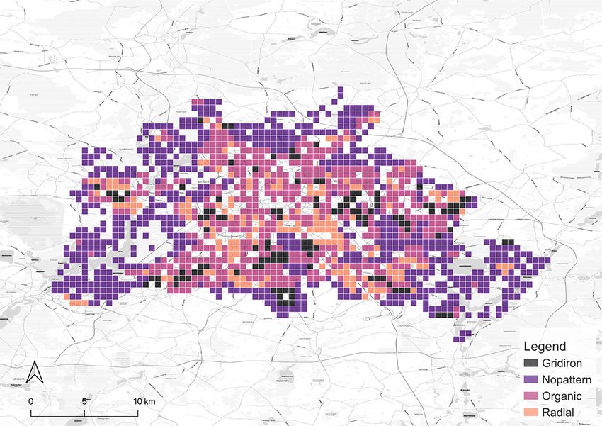
results including the performance of the models and the outcomes, followed by the in-
terpretation of the results. Section 5 discusses the results and describes limitations and
future studies. Section 6 concludes the paper.

2. Background and related work

2.1. Urban Morphology
    Novel methods and tools were developed to support studying urban morphology
(Fleischmann, 2019; Fleischmann et al., 2020; Jochem and Tatem, 2021). For exam-
ple, OSMnx provides an efficient way to acquire massive data of built environments
from OpenStreetMap and analyze them (Boeing, 2017). Boeing (2021) demonstrates a
workflow of its application on street pattern, orientation and configuration studies. With
these tools, it is now possible to analyze street networks across thousands of urban areas
(Boeing, 2020).
    Urban morphology characterized by morphological indices conveys quantities but
overlooks the pattern that could be grasped by eyes. The flourishing development of
deep learning techniques enables machines to get a humanlike perception of urban mor-
phology based on images. In this field, related research efforts have been carried out in
the microscale built environment. They concentrated on object detection or segmentation
of street view images to study street-level morphological features (Middel et al., 2019),
demographic make-up (Gebru et al., 2017), landscapes (Helbich et al., 2019; Kim et al.,
2021), walkability (Zhou et al., 2019), and neighborhood vitality (Wang and Vermeulen,
2020).
    However, very limited relevant studies are conducted in mesoscale or macroscale
urban form studies, and not many have focused on the orthogonal view instead of the
street view. For instance, a fully-connected neural network is applied to optimize urban
morphological indicators for intensive and sustainable development of urban blocks (Qu
et al., 2019). However, urban morphology is still measured by traditional indicators and
no information is extracted from the human perspective. To the best of our knowledge,
the research of Moosavi (2017) is the only one that adopts deep learning methods to
obtain morphological features from images of road networks. The work involves one
million cities and utilizes Convolutional Auto Encoder (CAE) to transform images of
road networks into urban vectors and further classifies the cities. However, the work was
not published in a peer-reviewed international scientific journal, and due to the usage of
an unsupervised learning method, the model was not given any human perception. Cou-
pled with the problem of excessive scale, the study suffers from low interpretability of
outcomes and disability of providing practical recommendations for urban morphology
design. All these drawbacks call for a more granular morphological study based on a su-
pervised deep learning method that can interpret morphology with human sense, which
we seek to accomplish in our research.

                                            4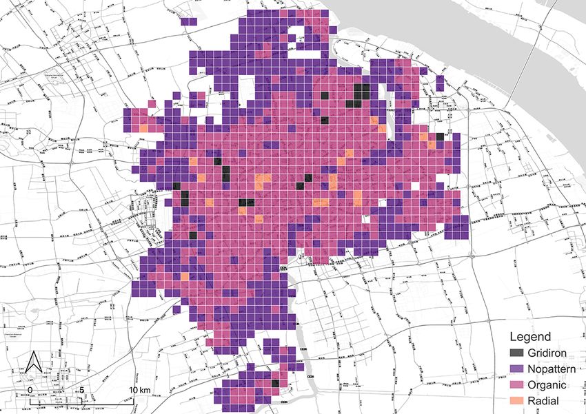
2.2. Urban Vitality
     Studies over the past several years include numerous big data-based methods to mea-
sure urban vitality from the perspective of built environment, density of people, and so
on.
     Points of interest (POI) is the most frequently used data source that describe the built
environment that supports human activities. Density of POI is a common indicator of
urban vitality, which is oftentimes supplemented by other indicators including density of
road junctions (Jin et al., 2017), housing prices and population change (He et al., 2018),
and other social-economic statistics (Zeng et al., 2018). Some research also reckons that
urban vitality can be gauged via small catering businesses (Xia et al., 2020; Ye et al.,
2018). They assume that the places where small catering businesses flourish tend to be
more vibrant because small catering businesses relied heavily on large flow of active
people.
     The density of people is in most cases measured by location-based services (LBS)
data. For example, social media check-ins are used to indicate the distribution of urban
vitality (Wu et al., 2018; Chen et al., 2019). Meng and Xing (2019) leverage place-based
reviews as an alternative. Yang et al. (2021) use the Baidu Heat Index (the density of
geographical locations of Baidu mobile application users) to represent urban vitality.
Further studies highlight the usage of mobile phone positioning data to portray urban
vitality (Yue et al., 2017; Li et al., 2020a). Besides, Kim (2018) adopts bankcard trans-
action data as the proxy of economic vitality and evaluated virtual vitality by Wi-Fi
access points.
     Nighttime light (NTL) data provides an additional approach to capture vitality. Such
data is proved to have a correlation with economic activities (Zhang and Seto, 2011; Ma
et al., 2014). Consequently, it is leveraged to detect “ghost cities” (cities with low urban
vitality) (Jin et al., 2017; Zheng et al., 2017; Ge et al., 2018), and delineate nighttime
urban vitality in street block level (Jin et al., 2017; Xia et al., 2020). Even though NTL
data has been testified somehow correlative with nighttime urban vitality, some reports of
its inconsistency with real human activities (Jin et al., 2017; Zhao et al., 2019) necessitate
the complement of other data sources.
     Some scholars attempt to evaluate urban vitality in a bigger picture. Landry (2000)
assumes that urban vitality is related to the economic, social, and physical environment.
Liu et al. (2010) build up a system that evaluates economic vitality, social vitality, cul-
tural vitality, and environmental vitality, supplemented by innovation vitality (Martino
et al., 2021). However, the data source they use often lacks granularity. Conveniently,
the advent of data sources such as WorldPop and Airbnb facilitates acquiring relevant
data with higher granularity (WorldPop, 2018; Tatem, 2017; Li and Biljecki, 2019). In
our study, overcoming the shortcomings of related work, we leverage these datasets as
new proxies of urban vitality.

                                              5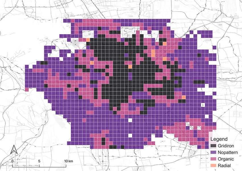
2.3. Urban Morphology and Urban Vitality
     The OLS regression model is the most commonly used method to analyze the re-
lationship between urban morphology and vitality. However, it suffers from two major
deficiencies: overlook of spatial relationship and excessive hypothesis of linearity. Some
effort has been made to rectify these issues. Spatial referenced models such as Local
Moran’s I statistics (Xia et al., 2020) and geographically weighted regression (GWR)
(Li et al., 2020a) have been adopted to alleviate the problem of ignoring the spatial rela-
tionship. However, the usage of nonlinear model is still an underexplored domain, and
another gap we seek to fill in this study. Morphological design in the future calls for
better evaluation of urban morphology’s influence on vitality. Nonlinear models qual-
ified with higher complexity are confirmed to be more accurate in urban study tasks
such as land use classification (Cao et al., 2019) and transportation mode classification
(Xiao et al., 2017). Among their model sets, XGBoost achieves the best performance.
LightGBM, which is also from the family of gradient boosting models, is a further im-
proved version proposed by Ke et al. (2017). LightGBM achieves further improvement
of training speed over XGBoost when inheriting most of its merits. Besides accuracy,
the identification of key morphological indices is also fundamental for the improvement
of urban morphology design in new constructions. As a tree-based model, LightGBM is
an appropriate approach enabling such competences. This study would for the first time
apply LightGBM to explore the relationship between urban morphology and vitality.

3. Methodology

3.1. Research Framework
3.1.1. Analytical framework
    Figure 1 illustrates the analytical framework of our work, which is composed of
three parts: measurement of urban morphology, measurement of urban vitality, and the
relationship between them.
    The first step is intended to measure urban morphology through two approaches, a
traditional one with morphological indices and a novel one we introduce, with road net-
work classification (inside the dashed box). Traditional morphological indices regard-
ing street, building and block are calculated by the Morphoindex generator, a Python
script developed for automatic generation of morphological indices, which we imple-
ment as part of this study. The geospatial datasets used in this study stem from two
main sources. One is OpenStreetMap (OSM), a Volunteered Geographic Information
(VGI) platform with global coverage and of high quality in many areas around the world
(Barrington-Leigh and Millard-Ball, 2017; Biljecki, 2020), and the others are the official
open datasets.
    Our proposed classification is conducted in three steps. First, we generate the im-
age of the road network legible for a computer. We develop a visual representation of
the road network called Colored Road Hierarchy Diagram (CRHD) and implement its
                                            6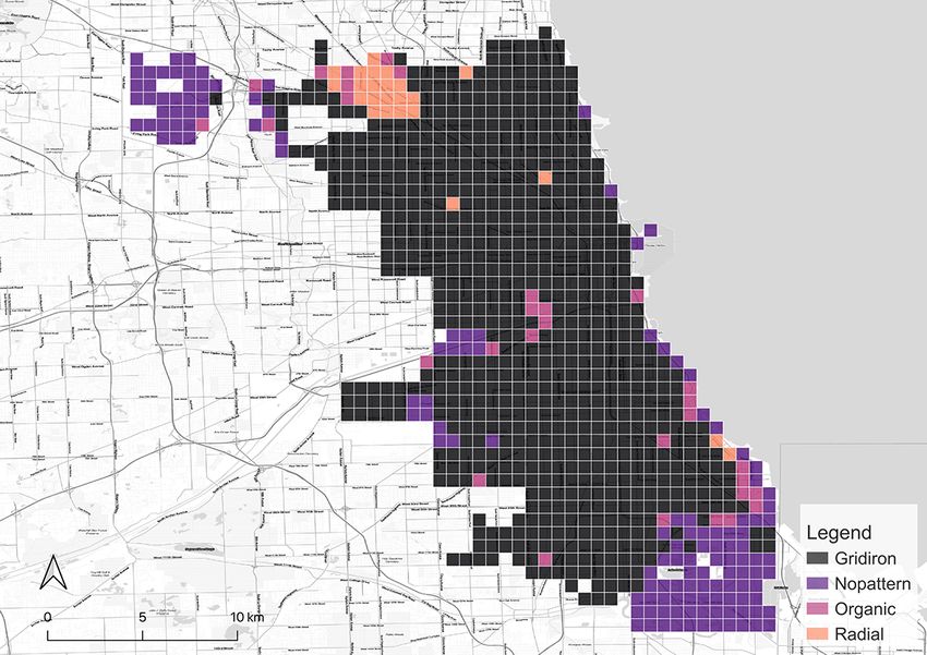
Figure 1: Analytical framework of our work.

generation in Python. The second step is to train the road network classification model,
which is based on the ResNet-34 architecture. A large group of CRHDs of representa-
tive urban zones are manually labelled and used for training. After training, the model
is able to calculate the probabilities of each road network category given an unlabeled
CRHD. With CRHDs classified based on the highest probability, we export categorical
maps at the city scale. The probabilities can be input into the feature space of quantita-
tive morphology studies as an augmentation. We maintain that it could inject simulated
human perceptions that are oftentimes ignored in the field.
     The effectiveness of the proposed method would be evaluated through a case study
of urban vitality prediction. Based on multi-source geospatial data, urban vitality is
assessed from five main aspects: built environment vibrancy measured by POI den-
sity, human activity density measured by tweet density, nighttime vibrancy measured by
nighttime light brightness, population density measured by population size, and tourism
vibrancy measured by density of Airbnb listings. This paper attaches equal importance
to all the five aspects, and they are expected to reduce the latent biases for each other.
We combine these indicators together as “vitality score” as a comprehensive evaluation
of urban vitality.
     The final portion of the paper aims to identify the correlation between urban mor-
phology and urban vitality. This study adopts LightGBM, a tree-based gradient boosting
method to delineate such relationships. Vitality score is used to evaluate the effective-
ness of road network classification. The evaluation is carried out through the comparison
among the metrics of a baseline model with only the traditional morphological indices
and an augmented model augmented with probabilistic indices. More nuanced relation-
                                              7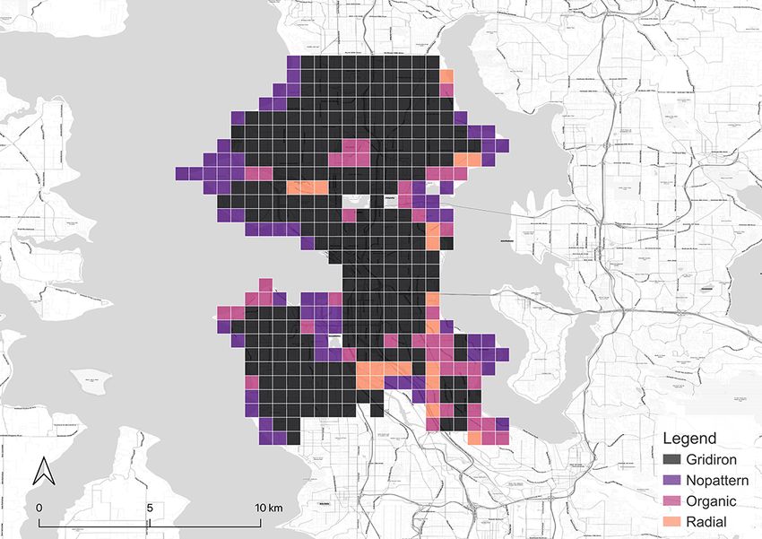
ships between the different aspects of vitality and urban morphology are also studied.

3.1.2. Study areas
     Considering the diversification of locations and similarity of development level, nine
cities spanning multiple continents are chosen as the study areas, including Singapore,
Shanghai, Beijing, New York, Chicago, Seattle, London, Paris, and Berlin. For the con-
venience of data collection and analysis, each city is latticed into approx. 1km × 1km
grids. The grids are in accordance with the 1km resolution grids from WorldPop (World-
Pop, 2018; Tatem, 2017; Lloyd et al., 2017, 2019). These grids contain their estimated
population inside, which is one of our indicators of urban vitality. Other indicators of
both urban vitality and morphology are processed to match the same grid system and
level.

3.2. Measurement of Urban morphology
3.2.1. Colored road hierarchy diagram
     A part of our method relies on OSMnx, a Python module developed by Boeing
(2017), which allows querying OpenStreetMap data in a programming environment. It
enables a straightforward generation of monochrome road network diagrams. This study
takes a step further. While monochrome road network diagrams represent road hierarchy
through visual thickness, we propose an improved version that represents road hierarchy
with both thickness and color. We name such sort of diagram Colored Road Hierarchy
Diagram (CRHD). We regroup the original road classes from OpenStreetMap into con-
densed five: motorway, primary roads, secondary roads, tertiary roads and minor roads.
Each class is specified a color and a thickness. A CRHD is generated through querying
the geospatial data of the road network in a given area through OSMnx and rendering
the roads based on our regroup and appearance rules. Thanks to the consistent standard
of OpenStreetMap data around the world, our generation method of CRHD is universal
and global. A Python script is developed as part of this study to carry out this generation
process, which we open-source.
     The colors of CRHDs aid the visual representation of road hierarchy and provides
an additional dimension of information to deep learning algorithms. Another merit of
CRHD is the convenience of conducting color thresholding to tone down a certain grade
of roads. For instance, minor roads which are in the lightest color can be erased by
truncating the pixels with high RGB values.
     Previous studies have proposed multiple divisions of road network categories (Snellen
et al., 2002; Plater-Zyberk et al., 2003; Marshall and Gong, 2005; Chan et al., 2011; Han
et al., 2020). Because our study covers cities around the world, universal suitability of
the taxonomy is important. Hence, we value the commonalities of the taxonomies. Ra-
dial, organic, and gridiron are found to be the three types that most frequently occur.
Additionally, we believe that these categories are easily discernible which is beneficial
to alleviate errors in manual labelling. We name these three categories “patterned road
                                            8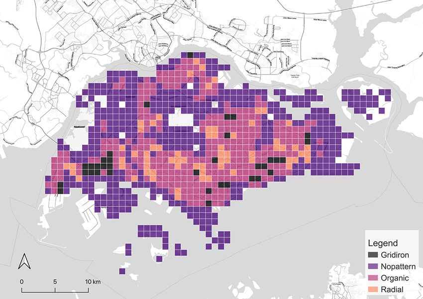
(a) Radial (Paris).    (b) Organic (Stuttgart).   (c) Gridiron (Chicago). (d) No pattern (London).

Figure 2: Quintessential CRHDs (2km × 2km) for different road network categories, as generated with our
tool. The underlying data is obtained from OpenStreetMap.

network categories” in comparison to another category we add — “no pattern”. The
intention of “no pattern” is to avoid misclassifying instances that do not belong to none
of the three patterned categories. As a result, the study employs four target categories.
The representative CRHDs for radial, organic, gridiron and no pattern are illustrated in
Figure 2.

3.2.2. ResNet-34
     ResNets, the abbreviation of Residual Neural Network, was first introduced by He
et al. (2015). Compared with common convolutional neural networks, ResNets reformu-
late the layers as learning the residual functions referring to the layer inputs. Compared
to earlier architectures such as VGGs, ResNets offer better performance per parameter
and faster inference speed (Canziani et al., 2016). ResNets are constructed by a series of
building blocks with “shortcuts”. In this paper, we use an improved scheme of building
blocks (He et al., 2016). After some preliminary experiments on model selection, this
study opts for ResNet-34.
     The task of the model is to classify the CRHDs into the given categories. Further, the
model is supposed to perceive the characteristics from a human’s view and convert this
information from an image to a feature vector. The paper employed the four probabilities
exported from the softmax layer as the embedded feature vector. The numbers in the
vector represent the probabilities of this CRHD belonging to each category.

3.2.3. Road network classification
    Figure 3 outlines the process of road network classification. It is implemented in two
steps. The blue arrows indicate the first section, which is the training of the road network
classification model. The training set include samples from our aforementioned study
area (20%) and also the other cities around the world (80%), which are 108 cities in
Asia, Europe, North America, and Africa in our case. Considering our limited capability
of manual labelling, the percentage is a trade-off between being more precise in given
areas and being more robust to unknown areas. We believe we choose the percentage
                                              9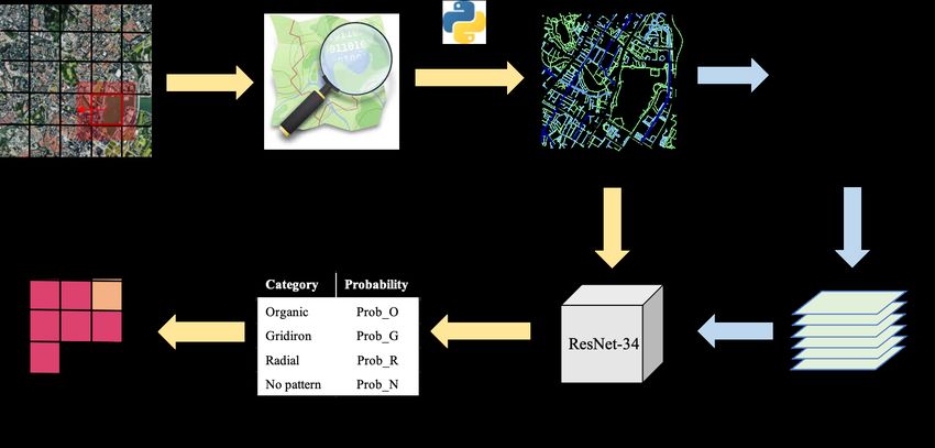
Figure 3: Process of road network classification.

that reconciles the model’s performance in our study area with its widespread applica-
tion. Training samples must possess a quintessential road network of one of the target
categories. The samples are fed to the road network classification model for training and
validating.
    The yellow arrows denote the second portion of the approach — the process of grid
road network classification. Avoiding unbuilt areas, the study excludes grids with no
buildings. The CRHDs used for prediction have a radius of 1km. It is worth noting that
the scale of a CRHD is twice as large as a grid. This difference in scale is under the
consideration of the interaction and conjunction of road networks among the adjacent
grids. It is unreasonable to take out one grid and study it separately without counting
the effect of the contextual road networks. Therefore, the CRHD is concentric with
the grid but with a doubled extent. Given an input of CRHD, the classification model
would return its probability of each category. Then the CRHD would be assigned to the
category with the highest probability. The probabilities could be further harnessed as
numerical morphological features in quantitative studies, while the categories could be
used for categorical analysis and the generation of the categorical maps for the cities.

3.2.4. Morphological Indices
     Urban morphology usually comprises three major components: street, building, and
block, which we follow in our study. We adopt the morphological indices reported cor-
relative to urban vitality in previous studies (Ye et al., 2018; Yang et al., 2021; Wu and
Niu, 2019; Bocher et al., 2018; Li et al., 2020a), including road density, intersection
density, building density, average building footprint area, block density, average block
area, and land use mixture. In addition to OpenStreetMap, in some cases we use of-
ficial open datasets from the municipal governments. After acquiring the shapefiles of
                                             10
street, building, and land use for each city, our Morphoindex generator is applied to re-
alise the aforementioned morphological indices automatically for each grid in the city.
Other than these traditional indices, the road network classification model provides four
probabilistic features as well. They are added into the feature space and regarded as sup-
plementation or augmentation of human sense, and they may also be seen as the level of
intensity of a particular form. The effectiveness of the augmentation is evaluated in the
following sections. The final list of morphological indices is shown in Table 1 with a
detailed description of each index. It is worthwhile to point out that the land use mixture
in a grid is gauged by Shannon entropy (Shannon, 1948), which describes the level of
uncertainty and mixture. It could be calculated through the following equation:
n
LUM = − ∑ pi log pi (1)
i=1
where n denotes the total amount of land use category in the grid, and pi is the proportion
of the area of ith category.
3.3. Measurement of urban vitality
This study inherits the frequently-used aspects of urban vitality from existing studies,
including built environment vibrancy, human activity density, and nighttime light bright-
ness. Two extra aspects of urban vitality, population density and tourism vibrancy are
supplemented. Table 2 shows the inventory of our urban vitality aspects, indicators and
data sources. Provided that each of those vitality indicators reflects only one character-
istic of urban vitality (human — tweet density, population; environment — POI density,
NTL, and Airbnb density), we define an indicator called “vitality score” that evaluates
the level of interactions (among humans and between human and environment) by inte-
grating our five vitality aspects. Vitality score ranges from 0 to 100. It is calculated by
three steps: (1) standardize the vitality indicators, (2) sum them up, and (3) rescale.
3.4. LightGBM
LightGBM (Ke et al., 2017) is a prevailing machine learning method in the in-
dustry, thanks to its fast speed, high accuracy, and ability to filter important features.
It is evolved from gradient boosting decision tree (GBDT). Given a training dataset
{(x1 , y1 ), (x2 , y2 ), · · · , (xn , yn )}, for each epoch, GBDT aims to find the best approxi-
mation fˆ to minimize the expectation of the loss function L(y, f (x)) (Eq. 2).
fˆ = arg min Ex,y [L(y, f (x))] (2)
f
Based on the idea of GBDT, LightGBM utilizes two new techniques, Exclusive Fea-
ture Bundling (EFB) and Gradient-based One-Side Sampling (GOSS), to accelerate the
training process and improve degree of accuracy.
11Table 1: Morphological indices incorporated in our study.
Component ID Name Description
Street Prob_R Probability of being radial Road network’s probability of
being radial
Prob_O Probability of being organic Road network’s probability of
being organic
Prob_G Probability of being gridiron Road network’s probability of
being gridiron
Prob_N Probability of being no pattern Road network’s probability of
being no pattern
RD Road density The total length of roads in a
grid divided by the area of the
grid
InD Intersection density The total number of intersec-
tions in a grid divided by the
area of the grid
Building BuD Building density The total area of building foot-
prints in a grid divided by the
area of the grid
ABFA Average building footprint area The average area of building
footprints in a grid
Block BlD Block density The total area of blocks in a grid
divided by the area of the grid
ABA Average block area Average area of blocks in a grid
LUM Land use mixture Shannon entropy of land use in
the grid
12Table 2: Urban vitality indicators and data sources.
Aspect Indicator Calculation Data source
Built environment vibrancy POI density Average kernel OpenStreetMap
density of POIs
Human activity density Tweet density Count of tweets Twitter Developer
API
Nighttime vibrancy NTL brightness Monthly average VIIRS DNB
NTL brightness
Population density Population size Estimated popula- WorldPop
tion
Tourism vibrancy Airbnb listing den- Average kernel Inside Airbnb
sity density of Airbnb
listing
In this study, we harnessed the Python package, lightgbm, to obtain an easy-to-use
application of the LightGBM model. As a tree-based model, LightGBM is capable
of ranking feature importance. The principle behind it roots from the process of the
generating decision trees. The importance of a feature could be evaluated through its
total number of times being selected for treenode split.
4. Results
4.1. Road network classification
The ResNet-34 was trained based on the labelled image set with 521 images, includ-
ing 136 gridiron samples, 163 organic samples, 82 images radial samples, and 140 no
pattern samples. The image set was randomly split into a training set with 432 images, a
validation set with 49 images and a testing set with 40 images (10 images for each cate-
gory). We truncated the minor roads (service roads, residential roads, etc.) from CRHDs
to eliminate noise. This method was proven to be useful in our trials. After parameter
tuning, the learning rate, batch size, and number of epochs was set to 0.0005, 2, and
30 respectively. The overall accuracy achieved in the testing set was 0.875. In contrast,
when using monochrome diagrams, the accuracy dropped to 0.75, affirming the value of
colored diagrams.
Figure 4 provides more detailed metrics such as the confusion matrix and the ROC
curves of the classification model. The diagonal of the confusion matrix (Figure 4(a))
denotes the accuracy of classification for each category. The model performed the best
in recognizing no pattern road networks and gridiron road networks with a hundred
13(a) Confusion matrix (b) ROC curves
Figure 4: Metrics for the road network classification model.
percent accuracy. The accuracy of classifying organic and radial road networks are rela-
tively lower which are 0.8 and 0.7, respectively. There are possible explanations for this
outcome. First, the classification of road networks relies heavily on the skeleton of ma-
jor roads as they are easier for the model to interpret. It is more advantageous for those
categories that are consistent in characteristics of major roads within the group such as
gridiron and no pattern. The major roads of the gridirons are in most cases consistent in
being straight and orthogonal, and no pattern road networks have rarely major roads. In
comparison, organic road networks have the winding and intertwined major roads which
create large blocks with irregular shapes, making it difficult to cover all kinds of sam-
ples. The characteristics of major roads of radial network are evident but very sensitive
to the position of the radial center in the image. The pattern of radial is distinct only if
the radial center locates near the center of the image. However, the grids from World-
Pop usually cannot capture the radial pattern properly, causing a decline in the accuracy.
Second, there is an unbalance for the sample size of the four categories in the image set.
Radial images were fewer than the counterparts due to fewer typical cases. This dispar-
ity also contributes to the final difference in accuracy. Although discrepancy of accuracy
among categories was found in the confusion matrix, the AUC values did not differ a lot
and were all above 0.9 (Figure 4(b)), indicating acceptable classification errors for all
the categories. Only the ROC curve of radial was slightly under the average ROC curve.
However, the model has been satisfactory enough.
After the model is all set, it is applied to classify the grids in all the cities in our focus.
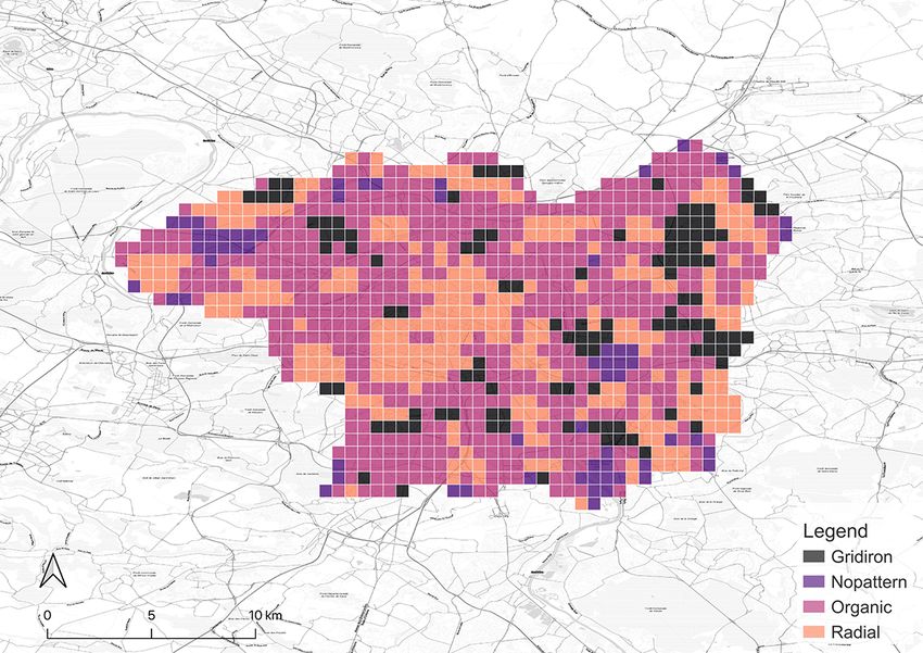
The results of the classification are shown in Figure 5. They are affirmed by well-known
facts, e.g. gridiron road network is a distinct common ground for North American cities
(Southworth and Ben-Joseph, 1995, 2013). Thus, locations in the US we selected, such
as New York City, Seattle, and Chicago have most of the grids identified as gridiron. The
last two are especially dominated by the gridiron pattern. New York City has obvious
14(a) Seattle (b) Chicago (c) London
(d) Paris (e) Berlin (f) Singapore
(g) New York (h) Beijing (i) Shanghai
Figure 5: Categorical maps of the cities derived from our classification method.
15gridiron road networks in the downtown areas such as Manhattan, Queens, and Brooklyn
while the outskirts are organic instead. Beijing fits a similar pattern. In contrast, a great
proportion of the downtown area in Paris is classified as radial in accordance with the
famous Parisian radial road structure, represented by the road network radiating from
the Triumphal Arch. London also has a considerable number of radial grids, but they
mainly distribute in the residential area outside the downtown core which is different
from the setting in Paris. It is worth noting that it is the organic pattern that takes the
largest portion in London and even in Paris. Another European city, Berlin, exhibits the
same structure. Akin to the preference on gridiron in North America, a commonality
of pattern in Europe seems to exist as well. Finally, the remaining two Asian cities,
Singapore and Shanghai, are predominantly organic-dominated.
Figure 6: Our classified results reveal clusters of urban form among the nine cities included in the study,
where the abscissa indicates the percentage of organic grids, the ordinate indicates the percentage of gridiron
instances, and the size of the point indicates the share of those that are radial.
Furthering the interpretation of the results, based on the commonalities of the pro-
portion of road network categories, the nine cities are clustered into four subgroups:
gridiron-dominated city (Chicago and Seattle), gridiron-organic-mixed city (New York
and Beijing), radial-organic-mixed city (London, Paris, and Berlin), and organic-dominated
city (Singapore and Shanghai). We can distinguish the subgroups as well in the scatter
plot (Figure 6). It should be noted that the number of no pattern grids detected in a city is
highly influenced by how much outskirt region of that city is included. Considering the
varying proportion of outskirts included among the cities, we exclude the grids with no
pattern in this analysis to prevent such variation from disturbing the result. This analysis
may be scaled to determine automatically the predominant urban form of thousands of
cities around the world.
164.2. Effectiveness of road network classification in predicting urban vitality
In this section, we proceed to assess the effectiveness of road network classification
in predicting urban vitality. The comparative assessment is conducted by comparing
the error metrics between a baseline model trained with only traditional morphological
indices and an augmented model trained with both traditional morphological indices and
probabilities of road network categories. In this study, we fine-tuned every LightGBM
model through a grid search technique with a 5-fold cross-validation.
Table 3: R-squared of vitality indicators obtained from two standardization strategies (standardization be-
fore and after merging).
POI density Tweet density NTL Population Airbnb Density
After merging 0.1270 -0.0762 0.1005 -0.0789 -0.2443
Before merging 0.5169 0.0202 0.3969 0.4394 0.2854
Before the training, standardization is necessary to handle the problem of outliers
and disparity of scale among the features. Since grids from different cities need to be
integrated, two standardization strategies are considered. The first strategy follows the
normal sequence, which is standardizing after the merging of data, while the second
one standardizes the data within each city before merging them together. LightGBMs
of each vitality indicator were trained in both strategies for comparison. The results
are shown in Table 3. We witness a substantial improvement of R-squared when we
standardize before merging. The R-squared of tweet density turned out to be low. Given
that another study reported a moderate association between urban morphology and tweet
density (Crooks et al., 2016), we attribute the contrasting result derived in our study to
the underdeveloped quality of the tweet data. We thus exclude tweet density in the
calculation of the vitality score. In another experiment, we discover higher R-squared
when targets are standardized as well. In the following experiments, the study would
conform to those standardization strategy.
Table 4: Comparison of error metrics between baseline model and augmented model, revealing the benefits
of our deep learning-based approach.
R squared RMSE MAE
Baseline model 0.5957 6.2139 4.0797
Augmented model 0.6227 6.0106 3.9611
The baseline model and the augmented model were then trained to fit the vitality
score based on their feature sets. The error metrics of the two models are shown in Ta-
ble 4. In contrast to the baseline model, there is a comprehensive improvement on all the
17metrics for the augmented model. Despite not being significant, it nevertheless indicates
a positive effect of the data augmentation provided by the road network classification
in terms of urban vitality prediction. We adopt the augmented model in the following
context.
4.3. Differences of morphology-vitality relationships among subgroups
This section aims to explore the possible differences of the relationship between ur-
ban morphology and vitality among the subgroups detected in Section 4.1. A model
involving all the studied cities was established in the first place to cast an overall insight
into the morphology-vitality relationship. The obtained R-squared for each vitality in-
dicator is visualized in Figure 7 (the blue bars). To better explain the results, the study
sets a criterion here. The relationships with the R-squared larger than 0.5, from 0.25 to
0.5, from 0 to 0.25 and equal to 0 (R-squared less than 0 would be reset to 0) would
be considered as high-level, medium-level, low-level, and not relative, respectively. The
results reveal that, in an overall context, urban morphology has a high-level relationship
with POI density, a medium-level relationship with NTL, population and Airbnb density,
but a very low-level relationship with Tweet density.
Figure 7: R-squared of vitality indicators for each subgroup.
To discover the potential discrepancy between different subgroups, LightGBM mod-
els for each subgroup were trained individually in the same process as the overall model.
The R-squared for each subgroup is plotted in the bar chart (Figure 7). The R-squared
of tweet density for all the groups are low, which is consistent with the observation
before. If we exclude this exception, we could observe the variation of the degree of
morphology-vitality relationship among the subgroups. The radial-organic-mixed cities
surpass the average R-squared and almost reached a high-level relationship in all aspects
of vitality. However, gridiron-organic-mixed cities are on the contrary. They achieve
lower R-squared in all the fields than the overall situation but still maintain medium-
level relationships in most fields except Airbnb density. Organic-dominated cities are
only detected a medium-level relationship with population with no other distinct rela-
tionship. Gridiron-dominated cities are also highly associated with population, and in
18the meantime have a medium-level relationship with NTL and a low-level relationship
with POI density. The difference among subgroups is substantial. It unveils that cities
in different subgroups (with different combination of patterned road network categories)
are likely to possess different morphology-vitality relationship.
4.4. Relationship between urban morphology and vitality at the grid scale
(a) POI density. (b) Tweet density. (c) NTL.
(d) Population. (e) Airbnb density. (f) Vitality score.
Figure 8: Feature importance plots of the overall model.
While we have presented the differences of morphology-vitality relationship in re-
gard to different subgroups of cities, this section focuses on the relationship between
urban morphology and vitality in grid scale. Figure 8 illustrates feature importance dia-
grams for the vitality score and the five vitality indicators of the corresponding models
trained on the grids of all candidate cities. In this case, feature importance of a feature is
calibrated by the number of times it is selected for splitting treenodes. As the total num-
ber of trees and treenodes vary from models, the absolute values of feature importance
also differed from models but it would not affect our interpretation. The most important
morphological features related to the POI density are building density, intersection den-
sity, and block density. For tweet density, because of its near-zero R-squared, its impor-
tance feature could be misleading. The NTL turns out to be tied strongly with building
density, average building footprint area and road density. Population and Airbnb den-
sity captures the strongest synergy with the probability of no pattern. Besides, building
density, block density are also high ranking features for them.
In conclusion, indicators regarding the development intensity (e.g. building density
and intersection density) play a vital role in nearly all aspects of vitality, whereas proba-
19Table 5: Mean, median, and standard deviation of vitality scores of road network categories.
Mean Median Standard deviation
Gridiron 20.69 17.80 11.05
Organic 19.46 17.38 9.80
Radial 19.10 16.58 9.89
No pattern 10.86 9.91 5.12
bilities of road network categories except for no pattern are in the opposite. Development
intensity is the key for urban vitality in a grid, while comparatively patterned road net-
work categories seem to matter not much. The feature importance diagram (Figure 8(f))
for the vitality score highlights analogous findings.
5. Discussion
5.1. Understanding the effectiveness of road network classification
Section 4.2 uncovers the small but positive effect of the road network classification.
We would discuss and explore the root of it. Table 5 lists the mean, median, and standard
deviation of the overall vitality scores for each road network category. It underscores a
clear gap of average vitality score between no pattern and the other categories. In con-
trast, the differences among the gridiron, organic, and radial grids are subtle. The kernel
density estimation (KDE) curves shown in Figure 9(a) corroborate the finding. There is
a clear left shift for the KDE curve of no pattern compared to the rests. Given that salient
correlations with the probability of no pattern exist for many aspects of vitality, it seems
that the improvement brought by the classification primarily contributes to identifying
urban areas without clear patterns.
To get a closer insight, we illustrate the proportion of each road network category
in different ranges of vitality score together with the number of instances in each range
in Figure 9(b). From the first range (0-20) to the third range (40-60), the proportion of
no pattern drops dramatically, making itself significant for the prediction. Meanwhile,
the percentages of the other three categories grow in a similar rate, which means the
differentiation among the three categories is trivial for the prediction. Given the fact that
most instances concentrate on the first three ranges, it explains why, in global statistics,
the probability of no pattern plays a role in urban vitality prediction while the rest three
do not.
The no-patterns are those whose road networks fail to articulate a pattern or formu-
late one as efficient as the three patterned ones (gridiron, organic, and radial), which
could root from manifold reasons. Subjective reasons could include locality in suburb,
lying on land use requiring sparse network, etc. Objective reasons could be encountering
20(a) Kernel density estimation curves. (b) Lines: proportion of each road network cate-
gory in ranges of vitality score. Bars: number of
instances in the range.
Figure 9: Distribution of vitality scores of four road network categories.
geographic obstacle such as hills, lakes and parks. The area fitting the above description
is relatively short of both human and activities. Also, the lack of well-structured net-
works causes less space for interaction and lower efficiency in all kinds of movements.
All these result in lower level of vitality in no pattern area. Thus, probability of no
pattern becomes helpful to urban vitality prediction.
5.2. The influence of urban morphology on urban vitality
According to the results and discussion presented earlier, globally, development in-
tensity is predominant in determining urban vitality, and the identification of no pattern
is the primary source of the effect of road network classification on urban vitality evalu-
ation.
However, we also observe some anomalies in Figure 9(b). We find that for the last
two ranges with high vitality score (60-80 and 80-100), gridiron and organic covers an
outright majority with the proportions of radial and no pattern approaching zero. The
story deviates from the original trend that the patterned categories evenly distribute the
proportion yielded from no pattern with the rising of vitality score. Instead, the relative
proportion among the patterned categories becomes more unbalanced especially for the
range 80-100. It means the probabilities of the patterned categories start to affect vitality
evaluation in a way when vitality score is very high. Whereas, due to the very limited
number of instances in these two ranges, the global statistics cannot capture and present
this feature.
We further explore the particular case by listing the average vitality score and mor-
phological indices of the top 10 vital instances for each patterned category (Table 6).
In high vitality context, the gridirons surpass the counterparts much further in vitality
score compared to the global case in Table 5. It should be noted that the radials keep
21Table 6: Average morphological indices and vitality scores of top 10 vibrant grids for each patterned road
network category.
Building Road Intersection Average Block Average Vitality
density density density block density building score
(%) (m/km2 ) (km−2 ) area (km−2 ) footprint
(m2 ) density
(m2 )
Gridiron 58 22444.9 704.5 24484.37 126.3 1816.3 89.65
Organic 50 19801.5 675.6 8700.7 460.2 759.10 77.68
Radial 68 22212.4 584.8 40982.33 44.4 980.27 57.27
the greatest building density whereas only achieve the lowest vitality score. In con-
trast, the gridirons and the organics keep lower building density but manage to maintain
higher level of urban vitality. The finding indicates these two road network categories,
especially gridiron may take advantage in the cultivation of extreme urban vitality. We
attempt to discuss the reason behind this according to the information from Table 6 and
urban planner’s intuition.
In gridiron road networks, most buildings are surrounded by four orthogonal roads,
so every facade of the buildings gets the opportunity to be interactive. Besides, the
intensive and orthogonal road network bring about more intersections, as is shown in
Table 6. The increasing number of intersections is beneficial to the efficient movement
of pedestrians and pave the way to incubate more human activities. All these advantages
enable gridiron road network to bear extreme urban vitality.
As for the organics, they shared the characteristic of curved major roads that split
the land into superblocks. Organic networks also expand the facades for interactions
by increasing the length of the roads via curvature. It provides less efficient space for
interactions than the gridirons, but requires less road density as well (Table 6). It makes
the organic a more economical option than the gridiron. The relatively stable high pro-
portion of organic in all ranges supports this statement (Figure 9(b)).
The radials have major roads from different directions converged at a central area,
enabling the center to reach the surrounding areas efficiently and vice versa. The move-
ment between blocks would more or less resort to the major network, which breeds
more interactions on the facades facing major roads but in turn discourages the vibrancy
of other areas. If the interactive facades of one radial structure are fully occupied, the
spillover vitality resources (people, POIs, etc.) would prefer to mitigate to a better posi-
tion elsewhere because of the comparative advantage. As a result, the vitality resources
would be dispensed and results in the difficulty in achieving high level of vitality.
225.3. Limitations and future studies
The study proposed a new method to classify road networks and managed to ful-
fil a high level of classification accuracy. However, there is still space for the model
to be ameliorated. First, the labelled image set still needs to be enriched with more
samples around the world to make the model more universally applicable. Second, the
model could recognize the overall pattern of the CRHDs well but not more detailed in-
formation. Object detection technique represented by Faster-RNN (Ren et al., 2016) and
YOLO (Redmon et al., 2016) could be an alternative solution. Instead of classifying
the road network pattern with a fixed scale, object detection models may detect the road
network patterns in variable scales within a larger CRHD, providing more information
for planners.
This study included a sufficient number of distinct cities to assess the approach.
Nevertheless, more cities should be involved in the future study for an all-round anal-
ysis. Conveniently, the process of generating a map of road network category such as
the ones in Figure 5 is automatic thanks to the CRHD generator and the road network
classification model that we presented in this paper. It means that it would not be too
complicated to add in more cities, which we seek to do in follow-up studies, potentially
creating a global repository of urban form data. With that, perhaps we could obtain
more conspicuous subgroups of road network categories. The difference between the
subgroups, which was only briefly discussed in this paper due to length limitations, is
also a topic worth digging deeper into.
A case study of urban vitality prediction was conducted in this paper to examine
the effectiveness of road network classification, yet that may not have been perfect to
confirm the effectiveness. Other case studies could also be made in the future with
the supplement of the road classification model proposed in this paper. For instance,
the influence of the road network category could be researched in other popular urban
study fields such as energy consumption, heat island, mobility, and so forth. This new
technique are expected to bring about more points of penetration in these research lines.
6. Conclusions
In this paper, we have presented a comprehensive and novel study investigating the
nascent application of deep learning in urban morphology, and one that brings advance-
ments also to research focusing on urban vitality. We highlight the following five key
contributions, findings, and takeaways of this study:
1. This research studied urban morphology from the perspective of road network
classification. It proposed Colored Road Hierarchy Diagram (CRHD), which is
easy to produce and beneficial for machine cognition. It offers an automatic
pipeline to obtain the predicted category and corresponding probabilities for a
road network, which offer several advantages over current approaches.
232. The study included the development of tools and models such as the Morphoindex
generator, CHRD generator, and road network classification model, and we release
them openly to facilitate future urban morphology studies.
3. Thanks to our approach, four subgroups were observed within the nine studied
cities in terms of the percentage distribution of each sort of road networks. The
approach is efficient and scalable, supporting large-scale comparative morpholog-
ical studies at the global scale.
4. Aided by LightGBM, the effect of road network classification was examined through
a case study of urban vitality prediction. The effect was small but positive. We de-
tected the source of the effect. The measurement of vitality involved more aspects
and data sources than previous studies.
5. Although development intensity was found the key factor of urban vitality glob-
ally, the study witnessed a possible role of road network categories in achieving
high-level vitality.
The deep learning-based method to quantify urban morphology, which is the core of
this paper, served as a road network classifier. It could output the probabilities of being
gridiron, organic, radial, and no pattern for an inputted CRHD. The main body of the
method was the road network classification model with the architecture of ResNet-34. It
managed to attain an overall accuracy of 0.875. CRHD was proven to be more legible for
machines. To some degree, we validated the potential capability of machines to perceive
and understand urban morphology as humans do. The method we proposed showcases
how to automate urban morphology study with supervised deep learning techniques.
We believe that the probabilities and categories obtained from the road classification
model could help to reap more comprehensive knowledge on urban morphology and its
impact on other urban study objects. In our case study, we compared the performances
between the baseline model and the augmented model in predicting overall urban vitality
score. We found that road network classification affects the vitality prediction positively
but only to some degree. The association between morphological indices and each as-
pect of urban vitality was studied as well. Built environment vibrancy turned out to be
the most relevant with urban morphology followed by population density and nighttime
vibrancy. The cross-group differences in the morphology-vitality relationships was also
discovered. Urban morphology of radial-organic-mixed cities is the most correlative
with urban vitality.
By analyzing the proportion of the road network categories in different ranges of
vitality score, we confirmed the derivation of the detected effect of road network classi-
fication, which is the differentiation of no pattern area. We also found and discussed the
possible disparity of ability to cultivate high level urban vitality among gridiron, organic
and radial. Gridiron and organic seems more suitable for achieving high-level of urban
vitality than radial. However, this result has not been fully proven in this study.
As a case study, the discussion on categorical urban morphology and urban vitality
in this paper sheds a light on not only the improvement of statistic metrics but also the
24You can also read