Recent Advances in 3D Object and Hand Pose Estimation
←
→
Page content transcription
If your browser does not render page correctly, please read the page content below
Recent Advances in 3D Object and Hand Pose Estimation

                                                                               Vincent Lepetit
                                                                           vincent.lepetit@enpc.fr
                                                  LIGM, Ecole des Ponts, Univ Gustave Eiffel, CNRS, Marne-la-Vallée, France

                                                                                             Abstract
arXiv:2006.05927v1 [cs.CV] 10 Jun 2020

                                                   3D object and hand pose estimation have huge potentials for Augmented Reality, to enable tan-
                                               gible interfaces, natural interfaces, and blurring the boundaries between the real and virtual worlds.
                                               In this chapter, we present the recent developments for 3D object and hand pose estimation using
                                               cameras, and discuss their abilities and limitations and the possible future development of the field.

                                         1    3D Object and Hand Pose Estimation for Augmented Reality

                                         An Augmented Reality system should not be limited to the visualization of virtual elements integrated
                                         to the real world, it should also perceive the user and the real world surrounding the user. As even
                                         early Augmented Reality applications demonstrated, this is required to provide rich user experience,
                                         and unlock new possibilities. For example, the magic book application developed by Billinghurst and
                                         Kazo [Billinghurst et al., 2001] and illustrated by Figure 1, shows the importance of being able to
                                         manipulate real objects in Augmented Reality. It featured a real book, from which virtual objects would
                                         pop up, and these virtual objects could be manipulated by the user using a small real “shovel”.
                                             This early system relied on visual markers on the real book and the shovel. These markers would
                                         become the core of the popular ARToolkit, and were essential to robustly estimate the locations and
                                         orientations of objects in the 3D space, a geometric information required for the proper integration of
                                         the virtual objects with the real book, and their manipulation by the shovel.
                                             Visual markers, however, require a modification of the real world, which is not always possible nor
                                         desirable in practice. Similarly, magnetic sensors have also been used to perceive the spatial positions of
                                         real objects, in order to integrate them to the augmented world. However, they share the same drawbacks
                                         as visual markers.
                                             Being able to perceive the user’s hands is also very important, as the hands can act as an interface
                                         between the user’s intention and the virtual world. Haptic gloves or various types of joysticks have been
                                         used to capture the hands’ locations and motions. In particular, input pads are still popular with current
                                         augmented and virtual reality platforms, as they ensure robustness and accuracy for the perception of
                                         the user’s actions. Entirely getting rid of such hardware is extremely desirable, as it makes Augmented
                                         Reality user interfaces intuitive and natural.
                                             Researchers have thus been developing Computer Vision approaches to perceiving the real world
                                         using simple cameras and without having to engineer the real objects with markers or sensors, or the
                                         user’s hands with gloves or handles. Such perception problem also appears in fields such as robotics,
                                         and the scientific literature on this topic is extremely rich. The goal of this chapter is to introduce the

                                                                                                 1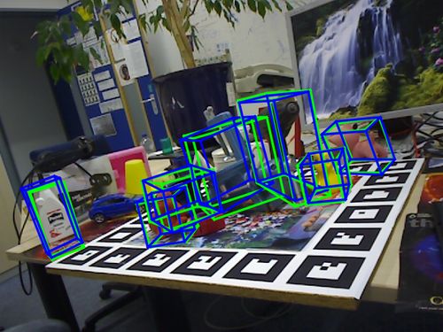
Figure 1: Augmented Reality (left) and external (right) views of the early Magic book developed by
Kazo and Billinghurst. This visionary experiment shows the importance of real object manipulation in
AR applications.

reader to 3D object and hand perception based on cameras for Augmented Reality applications, and to
the scientific literature on the topic, with a focus on the most recent techniques.
    In the following, we will first detail the problem of 3D pose estimation, explain why it is difficult, and
review early approaches to motivate the use of Machine Learning techniques. After a brief introduction
to Deep Learning, we will discuss the literature on 3D pose estimation for objects, hands, and hands
manipulating objects through representative works.

2    Formalization

In the rest of this chapter, we will define the 3D pose of a rigid object as its 3D location and orientation in
some coordinate system, as shown in Figure 2. In the case of Augmented Reality, this coordinate system
should be directly related to the headset, or to the tablet or smartphone, depending on the visualization
system, and to the object. This is thus different from Simultaneous Localization and Mapping (SLAM),
where the 3D pose of the camera can be estimated in an arbitrary coordinate system as long as it is
consistent over time.
    In general, this 3D pose has thus 6 degrees of freedom: 3 for the 3D translation, and 3 for the 3D
orientation, which can be represented for example with a 3D rotation matrix or a quaternion. Because
of these 6 degrees of freedom, the 3D pose is also called ’6D pose’ in the literature, the terms ’3D pose’
and ’6D pose’ thus refer to the same notion.
    Articulated objects, such as scissors, or even more deformable objects such as clothes or sheets of
papers have also been considered in the literature [Salzmann and Fua, 2010; Pumarola et al., 2018].
Their positions and shapes in space have many more degrees of freedom, and specific representations
of these poses have been developed. Estimating these values from images robustly remains very chal-
lenging.
    The 3D pose of the hand is also very complex, since we would like to also consider the positions of
the individual fingers. This is by contrast with gesture recognition for example, which aims at assigning
a distinctive label such as ’open’ or ’close’ to a certain hand pose. Instead, we would like to estimate
continuous values in the 3D space. One option among others to represent the 3D pose of a hand is
to consider the 3D locations of each joint in some coordinate system. Given a hand model with bone

                                                      2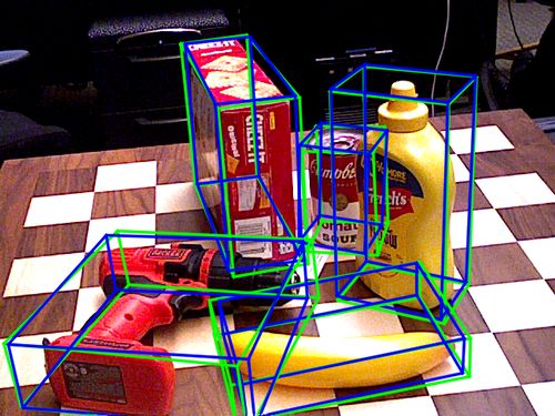
(a)                                                   (b)

Figure 2: (a) The 3D pose of a rigid object can be defined as a 3D rigid motion between a coordinate
system attached to the object and another coordinate system, for example one attached to an Augmented
Reality headset. (b) One way to define the 3D pose of a hand can be defined as a rigid motion between
a coordinate system attached to one of the joints (for example the wrist) and another coordinate system,
plus the 3D locations of the joints in the first coordinate system. 3D rigid motions can be defined as the
composition of a 3D rotation and a 3D translation.

length and rotation angles for all DoF of the joints, forward kinematics [Gustus et al., 2012] can be used
to calculate the 3D joint locations. Reciprocally, inverse kinematics [Tolani et al., 2000] can be applied
to obtain joint angles and bone length from the 3D joint locations. In addition, one may also want to
estimate the shapes of the user’s hands, such as their sizes or the thickness of the fingers.
     To be useful for Augmented Reality, 3D pose estimation has to run continuously, in real-time. When
using computer vision, it means that it should be done from a single image, or stereo images captured
at the same time, or RGB-D images that provide both color and depth data, maybe also relying on the
previous images to guide or stabilize the 3D poses estimations. Cameras with large fields of view help,
as they limit the risk of the target objects to leave the field of view compared to more standard cameras.
    Stereo camera rigs, made of two or more cameras, provide additional spatial information that can be
exploited for estimating the 3D pose, but make the device more complex and more expensive. RGB-D
cameras are currently a good trade-off, as they also provide, in addition to a color image, 3D information
in the form of a depth map, i.e.a depth value for each pixel, or at least most of the pixels of the color
image. “Structured light” RGB-D cameras measure depth by projecting a known pattern in infrared light
and capturing the projection with an infrared camera. Depth can then be estimated from the deformation
of the pattern. “Time-of-flight” cameras are based on pulsed light sources and measure the time a light
pulse takes to travel from the emitter to the scene and come back after reflection.
    With structured-light technology, depth data can be missing at some image locations, especially
along the silhouettes of objects, or on dark or specular regions. This technology also struggles to work
outdoor, because of the ambient infrared sunlight. Time-of-flight cameras is also disturbed outdoor,
as the high intensity of sunlight causes a quick saturation of the sensor pixels. Multiple reflections
produced by concave shapes can also affect the time-of-flight.
    But despite these drawbacks, RGB-D cameras remain however very useful in practice when they
can be used, and algorithms using depth maps perform much better than algorithms relying only on
color information—even though the gap is decreasing in recent research.

                                                    3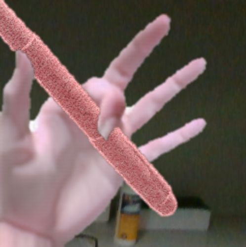
(a)                       (b)                            (c)

                              (d)                                              (e)

Figure 3: Some challenges when estimating the 3D poses of objects and hands. (a) Degrees of freedom.
The human hand is highly articulated, and many parameters have to be estimated to correctly represent
its pose. (b) Occlusions. In this case, the hand partially occludes the object, and the object partially
occludes the hand. (c) Self-occlusions can also occur in the case of hands, especially in egocentric
views. (d) Illuminations. Like the rubber duck in these examples, the appearance of objects can vary
dramatically with illumination. (e) Ambiguities. Many manufactured objects have symmetric or almost
symmetric shapes, which may make pose estimation ambiguous (object and images from the T-Less
dataset [Hodan et al., 2016]).

3    Challenges of 3D Pose Estimation using Computer Vision

There are many challenges that need to be tackled in practice when estimating the 3D poses of objects
and hands from images. We list below some of these challenges, illustrated in Figure 3.

High degrees of freedom. As mentioned above, the pose of a rigid object can be represented with
6 scalar values, which is already a large number of degrees of freedom to estimate. The 3D pose of a
human hand lives in an even much higher dimensional space, as it is often represented with about 32
degrees of freedom. The risk of making an error when estimating the pose increases with this number
of degrees of freedom.

Occlusions.      Occlusions of the target objects or hands, even partial, often disturb pose estimation
algorithms. It can be difficult to identify which parts are visible and which parts are occluded, and the
presence of occlusions may make pose estimation completely fail, or be very inaccurate. Occlusions
often happen in practice. For example, when a hand manipulates an object, both the hand and the object
are usually partially occluded.

Cluttered background. Objects in the background can act as distractors, especially if they look like
target objects, or have similar parts.

                                                    4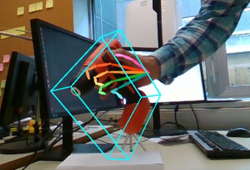
Changing illumination conditions. In practice, illumination cannot be controlled, and will change
the appearance of the objects, not only because the lighting is different but also because shadows can be
cast on them. This requires robust algorithms. Moreover, cameras may struggle to keep a good balance
between bright glares and dark areas, and using high dynamic range cameras becomes appealing under
such conditions. Moreover, sunlight may make depth cameras fail as discussed above.

Material and Textures. Early approaches to pose estimation relied on the presence of texture or
pattern on the objects’ surfaces, because stable features can be detected and matched relatively easily
and efficiently on patterns. However, in practice, many objects lack textures, making such approach
fail. Non-Lambertian surfaces such as metal and glass make the appearance of objects change with the
objects’ poses because of specularities and reflections appearing on the objects’ surfaces. Transparent
objects are also of course problematic, as they do not appear clearly in images.

Ambiguities. Many manufactured objects are symmetrical or almost symmetrical, or have repetitive
patterns. This generates possible ambiguities when estimating the poses of these objects that need to be
handled explicitly.

3D Model Requirement. Most of the existing algorithms for pose estimation assume the knowledge
of some 3D models of the target objects. Such 3D models provide very useful geometric constraints,
which can be exploited to estimate the objects’ 3D poses. However, building such 3D models takes
time and expertise, and in practice, a 3D model is not readily available. Hand pose estimation suffers
much less from this problem, since the 3D geometry of hands remains very similar from one person to
another. Some recent works have also considered the estimation of the objects’ geometry together with
their poses [Grabner et al., 2018]. These works are still limited to a few object categories, such as chairs
or cars, but are very interesting for future developments.

4    Early Approaches to 3D Pose Estimation and Their Limits

3D pose estimation from images has a long history in computer vision. Early methods were based on
simple image features, such as edges or corners. Most importantly, they strongly relied on some prior
knowledge about the 3D pose, to guide the pose estimation in the high-dimensional space of possible
poses. This prior may come from the poses estimated for the previous images, or could be provided by
a human operator.

3D tracking methods. For example, pioneer works such as [Harris and Stennett, 1990] and [Lowe,
1991] describe the object of interest as a set of 3D geometric primitives such as lines and conics, which
were matched with contours in the image to find a 3D pose estimate by solving an optimization problem
to find the 3D pose that reprojects the 3D geometric primitives to the matched image contours. The
entire process is computationally light, and careful implementations were able to achieve high frame
rates with computers that would appear primitive to us.
    Unfortunately, edge-based approaches are quite unreliable in practice. Matching the reprojection of
the 3D primitives with image contours is difficult to achieve: 3D primitives do not necessarily appear
as strong image contours, except for carefully chosen objects. As a result, these primitives are likely

                                                     5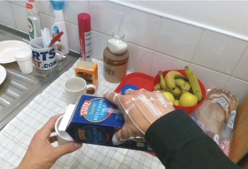
to be matched with the wrong image contours, especially in case of cluttered background. Incorrect
matches will also occur in case of partial occlusions. Introducing robust estimators into the optimization
problem [Drummond and Cipolla, 2002] helps, but it appears that it is impossible in general to be robust
to such mismatches in edge-based pose estimation: Most of the time, a match between two contours
provides only limited constraints on the pose parameters, as the two contours can “slide” along each
other and still be a good match. Contours thus do not provide reliable constraints for pose estimation.
    Relying on feature points [Harris and Stephens, 1988] instead of contours provides more constraints
as point-to-point matching does not have the “sliding ambiguity” of contour matching. Feature point
matching has been used for 3D object tracking with some success, for example in [Vacchetti et al.,
2004]. However, such approach assumes the presence of feature points that can be detected on the
object’s surface, which is not true for all the objects.

The importance of detection methods.            The two approaches described above assume that prior
knowledge on the object pose is available to guide the matching process between contours or points.
Typically, the object pose estimated at time t is exploited to estimate the pose at time t + 1. In practice,
this makes such approaches fragile, because the poses at time t and t + 1 can be very different if the
object moves fast, or because the pose estimated at time t can be wrong.
     Being able to estimate the 3D pose of an object without relying too much on prior knowledge is
therefore very important in practice. As we will see, this does not mean that methods based on strong
prior knowledge on the pose are not useful. In fact, they tend to be much faster and/or more accurate
than “detection methods”, which are more robust. A natural solution is thus to combine both, and this
is still true in the modern era of object and pose estimation.
    One early popular method for object pose estimation without pose prior was also based on feature
points, often referred to as keypoints in this context. This requires the ability to match keypoints between
an input image, and a reference image of the target object, which is captured offline and in which the
3D pose and the 3D shape of the object is known. By using geometry constraints, it is then possible
to estimate the object’s 3D pose. However, wide baseline point matching is much more difficult than
short baseline matching used by tracking methods. SIFT keypoints and descriptors [Lowe, 2001; Lowe,
2004] were a breakthrough that made many computer vision applications possible, including 3D pose
estimation. They were followed by faster methods, including SURF [Bay et al., 2008] and ORB [Rublee
et al., 2011].
    As for tracking methods based on feature points, the limitation of keypoint-based detection and pose
estimation is that it is limited to objects exhibiting enough keypoints, which is not the case in general.
This approach was still very successful for Augmented Reality in magazines for example, where the
“object” is an image printed on paper—so it has a simple planar geometry—and selected to guarantee
that the approach will work well by exhibiting enough keypoints [Kim et al., 2010].
    To be able to detect and estimate the 3D pose of objects with almost no keypoints, sometimes
referred to as “texture-less” objects, some works attempted to use “templates”: The templates of [Hin-
terstoisser et al., 2012b] aim at capturing the possible appearances of the object by discretizing the 3D
pose space, and representing the object’s appearance for each discretized pose by a template covering
the full object, in a way that is robust to lighting variations. Then, by scanning the input images looking
for templates, the target object can be detected in 2D and its pose estimated based on the template that
matches best the object appearance. However, such approach requires the creation of many templates,
and is poorly robust to occlusions.

                                                     6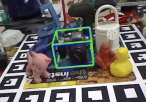
Conclusion. We focused in this section on object pose estimation rather than hand pose estimation,
however the conclusion would be the same. Early approaches were based on handcrafted methods to ex-
tract features from images, with the goal of estimating the 3D pose from these features. This is however
very challenging to do, and almost doomed to fail in the general case. Since then, Machine Learning-
based methods have been shown to be more adapted, even if they also come with their drawbacks, and
will be discussed in the rest of this chapter.

5    Machine Learning and Deep Learning

Fundamentally, 3D pose estimation of objects or hands can be seen as a mapping from an image to a
representation of the pose. The input space of this mapping is thus the space of possible images, which is
an incredibly large space: For example, a RGB VGA image is made of almost 1 million values of pixel
values. Not many fields deal with 1 million dimension data! The output space is much smaller, since it
is made of 6 values for the pose of a rigid object, or a few tens for the pose of a hand. The natures of
the input and output spaces of the mapping sought in pose estimation are therefore very different, which
makes this mapping very complex. From this point of view, we can understand that it is very difficult to
hope for a pure “algorithmic” approach to code this mapping.
    This is why Machine Learning techniques, which use data to improve algorithms, have become
successful for pose estimation problems, and computer vision problems in general. Because they are
data-driven, they can find automatically an appropriate mapping, by contrast with previous approaches
that required hardcoding mostly based on intuition, which can be correct or wrong.
    Many Machine Learning methods exist, and Random Forests, also called Random Decision Forests
or Randomized Trees, were an early popular method in the context of 3D pose estimation [Lepetit et al.,
2005; Shotton et al., 2013; Brachmann et al., 2014]. Random Forests can be efficiently applied to image
patches and discrete (multi-class) and continuous (regression) problems, which makes them flexible and
suitable to fast, possibly real-time, applications.

Deep Learning.         For multiple reasons, Deep Learning, a Machine Learning technique, took over
the other methods almost entirely during the last years in many scientific fields, including 3D pose
estimation. It is very flexible, and in fact, it has been known for a long time that any continuous mapping
can be approximated by two-layer networks, as finely as wanted [Hornik et al., 1989; Pinkus, 1999].
In practice, networks with more than two layers tend to generalize better, and to need dramatically less
parameters than two-layer networks [Eldan and Shamir, 2016], which makes them a tool of choice for
computer vision problems.
    Many resources can now be easily found to learn the fundamentals of Deep Learning, for example
[Goodfellow et al., 2016]. To stay brief, we can say here that a Deep Network can be defined as a
composition of functions (“layers”). These functions may depend on parameters, which need to be
estimated for the network to perform well. Almost any function can be used as layer, as long as it is
useful to solve the problem at hand, and if it is differentiable. This differentiable property is indeed
required to find good values for the parameters by solving an optimization problem.

Deep Network Training. For example, if we want to make a network F predict the pose of a hand
visible in an image, one way to find good values Θ̂ for the network parameters is to solve the following

                                                    7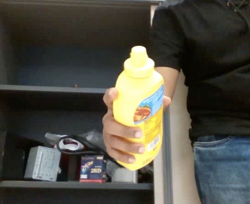
Figure 4: A basic Deep Network architecture applied to hand pose prediction. C1, C2, and C3 are
convolutional layers, P1 and P2 are pooling layers, and FC1, FC2, and FC3 are fully connected layers.
The numbers in each bar indicates either: The number and size of the linear filters in case of the convo-
lutional layers, the size of the pooling region for the pooling layers, and the size of the output vector in
case of the fully connected layers.

optimization problem:
                                      Θ̂ = arg minΘ L (Θ) with
                                                  N                                                      (1)
                                      L (Θ) = N1 ∑ kF(Ii ; Θ) − ei k2 ,
                                                 i=1

where {(I1 , e1 ), .., (IN , eN )} is a training set containing pairs made of images Ii and the corresponding
poses ei , where the ei are vectors that contain, for example, the 3D locations of the joints of the hand
as was done in [Oberweger et al., 2017]. Function L is called a loss function. Optimizing the network
parameters Θ is called training. Many optimization algorithms and tricks have been proposed to solve
problems like Eq. (1), and many software libraries exist to make the implementation of the network
creation and its training an easy task.
    Because optimization algorithms for network training are based on gradient descent, any differen-
tiable loss function can be used in principle, which makes Deep Learning a very flexible approach, as it
can be adapted easily to the problem at hand.

Supervised Training and the Requirement for Annotated Training Sets.                Training a network
by using a loss function like the one in Eq. 1 is called supervised training, because we assume the
availability of an annotated dataset of images. Supervised training tends to perform very well, and it is
used very often in practical applications.
    This is however probably the main drawback of Deep Learning-based 3D pose estimation. While
early methods relied only on a 3D model, and for some of them only on a small number of images of
the object, modern approaches based on Deep Learning require a large dataset of images of the target
objects, annotated with the ground truth 3D poses
   Such datasets are already available (see Section 6), but they are useful mostly for evaluation and
comparison purposes. Applying current methods to new objects requires creating a dataset for these
new objects, and this is a cumbersome task.

                                                       8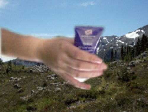
(a)                         (b)                       (c)                        (d)

Figure 5: Images from popular datasets for 3D object pose estimation. (a) LineMOD; (b) Occluded
LineMOD; (c) YCB-Video; (d) T-Less.

    It is also possible to use synthetic data for training, by generating images using Computer Graphics
techniques. This is used in many works, often with special to take into account the differences between
real and synthetic images, as we will see below.

6     Datasets

Datasets have become an important aspect of 3D pose estimation, for training, evaluating, and compar-
ing methods. We describe some for object, hand, and hand+object pose estimation below.

6.1   Datasets for Object Pose Estimation

LineMOD Dataset. The LineMOD dataset [Hinterstoisser et al., 2012b] predates most machine learn-
ing approaches and as such, it is not divided into a training and a test sets. It is made of 15 small objects,
such as a camera, a lamp, and a cup. For each object, it offers a set of 1200 RGB-D images of the object
surrounded by clutter. The other objects are often visible in the clutter, but only the 3D pose of the target
object is provided for each set. The 3D models of the objects are also provided.

Occluded LineMOD Dataset. The Occluded LineMOD dataset was created by the authors of [Brach-
mann et al., 2014] from LineMOD by annotating the 3D poses of the objects belonging to the dataset but
originally not annotated because they were considered as part of the clutter. This results into a sequence
of 1215 frames, each frame labeled with the 3D poses of eight objects in totla, as well as the objects’
masks. The objects show severe occlusions, which makes pose estimation challenging.

YCB-Video Dataset.         This dataset [Xiang et al., 2018a] consists of 92 video sequences, where 12
sequences are used for testing and the remaining 80 sequences for training. In addition, the dataset
contains 80k synthetically rendered images, which can be used for training as well. There are 21 “daily
life” objects in the dataset, from cereal boxes to scissors or plates. These objects were selected from
the YCB dataset [Calli et al., 2017] and are available for purchase. The dataset is captured with two
different RGB-D sensors. The test images are challenging due to the presence of significant image
noise, different illumination levels, and large occlusions. Each image is annotated with the 3D object
poses, as well as the objects’ masks.

                                                      9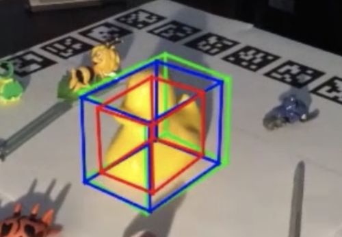
T-Less Dataset. The T-Less dataset [Hodan et al., 2016] is made from 30 “industry-relevant” objects.
These objects have no discriminative color nor texture. They present different types of symmetries and
similarities between them, making pose estimation often almost ambiguous. The images were captured
using three synchronized sensors: two RGB-D cameras, one structured-light based and one time-of-
flight based, and one high-resolution RGB camera. The test images (10K from each sensor) are from
20 scenes with increasing difficulties, with partial occlusions and contacts between objects. This dataset
remains extremely challenging.

6.2   Datasets for Hand Pose Estimation

Early datasets. The NYU dataset [Tompson et al., 2014] contains over 72k training and 8k test RGB-
D images data, captured from three different viewpoints using a structured-light camera. The images
were annotated with 3D joint locations with a semi-automated approach, by using a standard 3D hand
tracking algorithm reinitialized manually in case of failure. The ICVL dataset [Tang et al., 2014] con-
tains over 180k training depth frames showing various hand poses, and two test sequences with each
approximately 700 frames, all captured with a time-of-flight camera. The depth images have a high
quality with hardly any missing depth values and sharp outlines with little noise. Unfortunately, the
hand pose variability of this dataset is limited compared to other datasets, and annotations are rather in-
accurate [Supancic et al., 2015]. The MSRA dataset [Sun et al., 2015] contains about 76k depth frames,
captured using a time-of-flight camera from nine different subjects.

BigHands Dataset.       The BigHands dataset [Yuan et al., 2017] contains an impressive 2.2 millions
RGB-D images captured with a structured-light camera. The dataset was automatically annotated by
using six 6D electromagnetic sensors and inverse kinematics to provide 21 3D joint locations per frame.
A significant part is made of egocentric views. The depth images have a high quality with hardly any
missing depth values, and sharp outlines with little noise. The labels are sometimes inaccurate because
of the annotation process, but the dataset has a large hand pose variability, from ten users.

CMU Panoptic Hand Dataset. The CMU Panoptic hand dataset [Simon et al., 2017] is made of 15k
real and synthetic RGB images, from a third-person point of view. The real images were recorded in the
CMU’s Panoptic studio and annotated by the method proposed in the paper, based on multiple views.
The annotations are only in 2D but can still be useful for multi-view pose estimation.

6.3   Datasets for Object and Hand Pose Estimation

GANerated Hand Dataset. The GANerated hand dataset [Mueller et al., 2018b] is a large dataset
made of 330K synthetic images of hands, sometimes holding an object, in front of a random background.
The images are annotated with the 3D poses of the hand. The images were made more realistic by
extending CycleGAN [Zhu et al., 2017].

First-Person Hand Action dataset. The First-Person Hand Action dataset [Garcia-Hernando et al.,
2018] provides a dataset of hand and object interactions with 3D annotations for both hand joints and
object pose. They used a motion capture system made of magnetic sensors attached to the user’s hand
and to the object in order to obtain hand 3D pose annotations in RGB-D video sequences. Unfortunately,

                                                    10
(a) (b) (c)
(d) (e) (f)
Figure 6: Images from popular datasets for 3D hand (a) and hand+object (b-f) pose estimation. (a)
BigHand; (b) GANerated hand dataset; (c) First-Person Hand Action dataset; (d) Obman dataset; (e)
FreiHAND dataset; (f) HO-3D dataset.
this changes the appearance of the hand in the color images as the sensors and the tape attaching them
are visible, but the dataset proposes a large number of frames under various conditions (more than 100K
egocentric views of 6 subjects doing 45 different types of daily-life activities).
ObMan Dataset. Very recently, [Hasson et al., 2019a] introduced ObMan, a large dataset of images
of hands grasping objects. The images are synthetic, but the grasps are generated using an algorithm
from robotics and the grasps still look realistic. The dataset provides the 3D poses and shapes of the
hand as well as the object shapes.
FreiHand Dataset. [Zimmermann et al., 2019] proposed a multi-view RGB dataset, FreiHAND,
which includes hand-object interactions and provides the 3D poses and shapes of the hand. It relies on a
green-screen background environment so that it is easy to change the background for training purposes.
HO-3D Dataset. [Hampali et al., 2020] proposed a method to automatically annotate video se-
quences captured with one or more RGB-D cameras with the object and hand poses and shapes. This
results in a dataset made of 75,000 real RGB-D images, from 10 different objects and 10 different users.
The objects come from the YCB dataset (see Section 6.1). The backgrounds are complex, and the
mutual occlusions are often large, which makes the pose estimation realistic but very challenging.
116.4 Metrics
Metrics are important to evaluate and compare methods. Many metrics exist, and we describe here only
the main ones for object pose estimation. Discussions on metrics for 3D object pose estimation can be
found in [Hodan et al., 2016] and [Brégier et al., 2018].
ADD, ADI, ADD-S, and the 6D Pose metrics. The ADD metric [Hinterstoisser et al., 2012a] calcu-
lates the average distance in 3D between the model points, after applying the ground truth pose and the
predicted pose. This can be formalized as:
1
ADD = ∑ kTr(M; p̂) − Tr(M; p̄)k2 , (2)
|V | M∈V
where V is the set of the object’s vertices, p̂ the estimated pose and p̄ the ground truth pose, and Tr(M; p)
the rigid transformation in p applied to 3D point M. In the 6D Pose metric, a pose is considered when
the ADD metric is less than 10% of the object’s diameter.
For the objects with ambiguous poses due to symmetries, [Hinterstoisser et al., 2012a] replaces the
ADD metric by the ADI metric, also referred to as the ADD-S metric in [Xiang et al., 2018b], computed
as follows:
1
ADD-S = min kTr(M1 ; p̂) − Tr(M2 ; p̄)k2 , (3)
|V | M∑∈V 2
M ∈V
1
which averages the distances from points after applying the predicted pose to the closest points under
the ground truth pose. The advantage of this metric is that it is indeed equal to zero when the pose is
retrieved up to a symmetry, even if it does not exploit the symmetries of the object.
7 Modern Approaches to 3D Object Pose Estimation
Over the past years, many authors realise that Deep Learning is a powerful tool for 3D object pose
estimation from images. We discuss here the development of Deep Learning applied to 3D object
pose estimation over time. This development was and is still extremely fast, with improving accuracy,
robustness, and computation times. We present this development through several milestone methods,
but much more methods could also be included here.
7.1 BB8
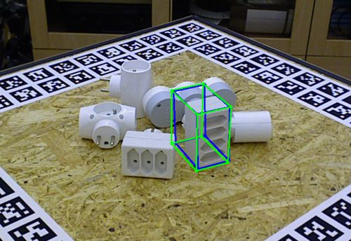
One of the first Deep Learning methods for 3D object pose estimation is probably BB8 [Rad and Lepetit,
2017]. As it is the first method we describe, we will present it in some details.
This method proceeds in three steps. It first detect the target objects in 2D using coarse object
segmentation. It then applies a Deep Network on each image window centered on detected objects.
Instead of predicting the 3D pose of the detected objects in the form of a 3D translation and a 3D
rotation, it predict the 2D projections of the corners of the object’s bounding box, and compute the 3D
pose from these 2D-3D correspondences with a PnP algorithm [Gao et al., 2003]—hence the name for
the method, from the 8 corners of the bounding box, as illustrating in Figure 7. Compared to the direct
prediction of the pose, this avoids the need for a meta-parameter to balance the translation and rotation
12Figure 7: Some 3D object pose estimation methods predict the pose by first predicting the 2D repro-
jections mi of some 3D points Mi , and then computing the 3D rotation and translation from the 2D-3D
correspondences between the mi and Mi points using a PnP algorithm.
terms. It also tends to make network optimization easier. This representation was used in some later
works.
Since it is the first Deep Learning method for pose estimation we describe, we will detail the loss
function (see Section 5) used to train the network. This loss function L is a least-squares error between
the predicted 2D points and the expected ones, and can be written as:
1
L (Θ) = ∑
8 (W,p)∈ ∑ kProjp (Mi ) − F(W ; Θ)i k2 , (4)
T i
where F denotes the trained network and Θ its parameters. T is a training set made of image windows W
containing a target object under a pose p. The Mi are the 3D coordinates of the corners of the bounding
box of for this object, in the object coordinate system. Proje,t (M) projects the 3D point M on the image
from the pose defined by e and t. F(W ; Θ)i returns the two components of the output of F corresponding
to the predicted 2D coordinates of the i-th corner.
The problem of symmetrical and “almost symmetrical” objects. Predicting the 3D pose of objects
a standard least-squares problem, using a standard representation of the pose or point reprojections as
in BB8, yields to large errors on symmetrical objects, such as many objects in the T-Less dataset (Fig-
ure 5(d)). This dataset is made of manufactured objects that are not only similar to each other, but also
have one axis of rotational symmetry. Some objects are not perfectly symmetrical but only because of
small details, like a screw.
The approach described above fails on these objects because it tries to learn a mapping from the
image space to the pose space. Since two images of a symmetrical object under two different poses look
identical, the image-pose correspondence is in fact a one-to-many relationship.
For objects that are perfectly symmetrical, [Rad and Lepetit, 2017] proposed a solution that we will
not describe here, as simpler solutions have been proposed since. Objects that are “almost symmetrical”
can also disturb pose prediction, as the mapping from the image to the 3D pose is difficult to learn
even though this is a one-to-one mapping. Most recent methods ignore the problem and consider that
these objects are actually perfectly symmetrical and consider a pose recovered up to the symmetries as
13Figure 8: Pose refinement in BB8. Given a first pose estimate, shown by the blue bounding box, BB8
generates a color rendering of the object. A network is trained to predict an update for the object pose
given the input image and this rendering, to get a better estimate shown by the red bounding box. This
process can be iterated.
correct. For such object, BB8 proposes to first consider these objects as symmetrical, and then to train
a classifier (also a Deep Network) to predict which pose is actually the correct one. For example, for an
object with a rotational symmetry of 180◦ , there are two possible poses in general, and the classifier has
to decide between 2 classes. This is a much simpler problem than predicting 6 degrees-of-freedom for
the pose, and the classifier can focus on the small details that break the symmetry.
Refinement step. The method described above provides an estimate for the 3D pose of an object
using only feedforward computation by a network from the input image to the 3D pose. It is relatively
natural to aim at refining this estimate, which is a step also present in many other methods. In BB8, this
is performed using a method similar to the one proposed in [Oberweger et al., 2015] for hand detection
in depth images. A network is trained to improve the prediction of the 2D projections by comparing the
input image and a rendering of the object for the initial pose estimate, as illustrated in Figure 8. Such
refinement can be iterated multiple times to improve the pose estimate.
One may wonder why the refinement step, in BB8 but also in more recent works such as DeepIM [Xi-
ang et al., 2018b] or DPOD [Zakharov et al., 2019], can improve pose accuracy while it is (apparently)
trained with the same data as the initial pose prediction. This can be understood by looking more closely
at how the network predicting the update is trained. The input part of one training sample is made of a
regular input image, plus an rendered image for a pose close to the pose for input image, and the output
part is the difference between the two poses. In practice, the pose for the rendered image is taken as
the ground truth pose for the real image plus some random noise. In other words, from one sample of
the original dataset trained to predict the network providing the first estimate, it is possible to generate
a virtually infinite number of samples for training the refinement network, by simply adding noise to
the ground truth pose. The refinement network is thus trained with much more samples than the first
network.
Data augmentation. Data augmentation, i.e. generating additional training images from the available
ones, is often critical in Deep Learning. In the case of BB8, the objects’ silhouettes are extracted from
14(a) (b)
Figure 9: (a) The architecture of SSD, extended by SSD-6D to predict 3D poses. For each bounding
box corresponding to a detected object, a discretized 3D pose is also predicted by the network. Image
from [Kehl et al., 2017]. (b) The architecture of YOLO-6D. Image from [Tekin et al., 2018].
the original training images, which can be done using the ground truth poses and the objects’ 3D models.
The background is replaced by a patch extracted from a randomly picked image from the ImageNet
dataset [Russakovsky et al., 2015]. Note that this procedure removes context by randomly replacing
the surroundings of the objects. Some information is thus lost, as context could be useful for pose
estimation.
7.2 SSD-6D
BB8 relies on two separate networks to first detect the target objects in 2D and then predict their 3D
poses, plus a third one if refinement is performed. Instead, as shown in Figure 9(a), SSD-6D [Kehl et
al., 2017] extends a deep architecture (the SSD architecture [Liu et al., 2016]) developed for 2D object
detection to 3D pose estimation (referred in the paper as 6D estimation). SSD had already been extended
to pose estimation in [Poirson et al., 2016], but SS6-6D performs full 3D pose prediction.
This prediction is done by first discretizing the pose space. Each discretized pose is considered
as a class, to turn the pose prediction into a classification problem rather than a regression one, as
this was performing better in the authors’ experience. This discretization was done on the 3D pose
decomposition into direction of view over a half-sphere and in-plane rotation. The 3D translation can
be computed from the 2D bounding box. To deal with symmetrical objects, views on the half-sphere
corresponding to identical appearance for the object are merged into the same class.
A single network is therefore trained to perform both 2D object detection and 3D pose prediction,
using a single loss function made of a weighted sum of different terms. The weights are hyperparameters
and have to be tuned, which can be difficult. However, having a single network is an elegant solution,
and more importantly for practical applications, this allows to save computation times: Image feature
extraction, the slowest part of the network, is performed only once even if it is used to predict the 2D
bounding boxes and the 3D pose estimation.
A refinement procedure is then run on each object detection to improve the pose estimate predicted
by the classifier. SSD-6D relies on a method inspired by an early approach to 3D object tracking based
on edges [Drummond and Cipolla, 2002]. Data augmentation was done by rendering synthetic views of
the objects using their 3D models over images from COCO [Lin et al., 2014], which helps but only to
some extend as the differences between the real and synthetic images (the “domain gap”) remain high.
15Figure 10: The architecture of PoseCNN. Image from [Xiang et al., 2018b].
7.3 YOLO-6D
The method proposed in [Tekin et al., 2018], sometimes referred as YOLO-6D, is relatively similar to
SSD-6D, but makes different choices that makes it faster and more accurate. As shown in Figure 9(b),
it relies on the YOLO architecture [Redmon et al., 2016; Redmon and Farhadi, 2017] for 2D object
detection, and predicts the 3D object poses in a form similar to the one of BB8. The authors report that
training the network using this pose representation was much simpler than when using quaternions to
represent the 3D rotation. As YOLO is much faster and as they do not discretize the pose space, [Tekin
et al., 2018] also reports much better performance than SSD-6D in terms of both computation times and
accuracy.
7.4 PoseCNN
PoseCNN is a method proposed in [Xiang et al., 2018b]. It relies on a relatively complex architecture,
based on the idea of decoupling the 3D pose estimation task into different sub-tasks. As shown in
Figure 10, this architecture predicts for each pixel in the input image 1) the object label, 2) a unit vector
towards the 2D object center, and 3) the 3D distance between the object center and the camera center,
plus 4) 2D bounding boxes for the objects and 5) a 3D rotation for each bounding box in the form of
a quaternion. From 1), 2), and 3), it is possible to compute the 3D translation vector for each visible
object, which is combined with the 3D rotation to obtain the full 3D pose for each visible object.
Maybe the most interesting contribution of PoseCNN is the loss function. It uses the ADD metric
as the loss (see Section 6.4), and even more interestingly, the paper shows that the ADD-S metric, used
to evaluate the pose accuracy for symmetrical objects (see Section 6.1), can be used as a loss function to
deal with symmetrical objects. The ADI metric makes use of the min operator, which makes it maybe
an unconventional loss function, but it is still differentiable and can be used to train a network. This
results in an elegant and efficient way of handling object symmetries.
16Figure 11: The DeepIM [Xiang et al., 2018b] refinement architecture. It is similar to the one of
BB8 (Figure 8) but predicts a pose update in a carefully chosen coordinate system for better generaliza-
tion.
Another contribution of [Xiang et al., 2018b] is the introduction of the YCB-Video dataset (see
Section 6.1).
7.5 DeepIM
DeepIM [Li et al., 2018] proposes a refinement step that resembles the one in BB8 (see the discussion
on refinement steps in Section 7.1), but with several main differences. As BB8, it trains a network to
compare the input image with a rendering of an object that has already been detected, and for which
a pose estimate is already available. The network outputs an update for the 3D object pose that will
improve the pose estimate, and this process can be iterated until convergence. The first difference with
BB8 is that the rendered image has a high-resolution and the input image is centered on the object and
upscaled to the same resolution. This allows a higher precision when predicting the pose update. The
loss function also includes terms to make the network output the flow and the object mask, to introduce
regularization.
The second difference is more fundamental, as it introduces a coordinate system well suited to define
the rotation update that must be predicted by the network. The authors first remark that predicting the
rotation in the camera coordinate system because this rotation would also translate the object. They
thus set the center of rotation to the object center. For the axes of the coordinate system, the authors
remark that using those of the object’s 3D model is not a good option, as they are arbitrary and this
would force the network to learn them for each object. They therefore propose to use the axes of the
camera coordinate system, which makes the network generalize much better. The translation update
is predicted as a 2D translation on the image plane, plus a delta along the z axis of the camera in a
log-scale. To learn this update, DeepIM uses the same loss function as [Xiang et al., 2018b] (ADD, or
ADD-S for symmetrical objects). This approach is even shown to generalize to unseen objects, but this
is admittedly demonstrated in the paper only on very simple object renderings.
17Figure 12: Autoencoders trained to learn an image embedding. This embedding is robust to nuisances
such as background and illumination changes, and the possible rotations for the object in the input image
can be retrieved based on this embedding. Image from [Sundermeyer et al., 2019].
7.6 Augmented Autoencoders
The most interesting aspect of the Augmented Autoencoders method proposed in [Sundermeyer et al.,
2019] is the way it deals with symmetrical objects. It proposes to first learn an embedding that can
be computed from an image of the object. This embedding should be robust to imaging artefacts (il-
lumination, background, etc.) and depends only on the object’s appearance: The embeddings for two
images of the object under ambiguous rotations should thus be the same. At run-time, the embedding
for an input image can then be mapped to all the possible rotations. This is done efficiently by creating a
codebook offline, by sampling views around the target objects, and associating the embeddings of these
views to the corresponding rotations. The translation can be recovered from the object bounding box’
2D location and scale.
To learn to compute the embeddings, [Sundermeyer et al., 2019] relies on an autoencoder architec-
ture, shown in Figure 12. An Encoder network predicts an embedding from an image of an object with
different image nuisances; a Decoder network takes the predicted embedding as input and should gener-
ate the image of the object under the same rotation but without the nuisances. The encoder and decoder
are trained together on synthetic images of the objects, to which nuisances are added. The loss function
encourages the composition of the two networks to output the original synthetic images, despite using
the images with nuisances as input. Another motivation for this autoencoder architecture is to learn to
be robust to nuisances, even though a more standard approach outputting the 3D pose would probably
do the same when trained on the same images.
7.7 Robustness to Partial Occlusions: [Oberweger et al., 2018], [Hu et al., 2019], PVNet
[Oberweger et al., 2018], [Hu et al., 2019], and PVNet [Peng et al., 2019] developed almost in parallel
similar methods that provide accurate 3D poses even under large partial occlusions. Indeed, [Oberweger
et al., 2018] shows that Deep Networks can be robust to partial occlusions when predicting a pose from
18Figure 13: Being robust to large occlusions. [Hu et al., 2019] makes predictions for the 2D reprojections
of the objects’ 3D bounding boxes from many image locations. Image locations that are not occluded
will result in good predictions, the predictions made from occluded image locations can be filtered out
using a robust estimation of the pose. Image from [Hu et al., 2019].
a image containing the target object when trained on examples with occlusions, but only to some extend.
To become more robust and more accurate under large occlusions, [Oberweger et al., 2018; Hu et al.,
2019; Peng et al., 2019] proposed to predict the 3D pose in the form of the 2D reprojections of some
3D points as in BB8, but by combining multiple predictions, where each prediction is performed from
different local image information. As shown in Figure 13, the key idea is that local image information
that is not disturbed by occlusions will result into good predictions; local image information disturbed
by occlusions will predict erroneous reprojections, but these can be filtered out with a robust estimation.
[Oberweger et al., 2018] predicts the 2D reprojections in the form of heatmaps, to handle the am-
biguities of mapping between image locations and the reprojections, as many image locations can look
the same. However, this makes predictions relatively slow. Instead, [Hu et al., 2019] predicts a single
2D displacement between the image location and each 2D reprojection. These results in many possible
reprojections, some noisy, but the correct 3D pose can be retrieved using RANSAC. PVNet [Peng et al.,
2019] chose to predict the directions towards the reprojections, rather than a full 2D displacement, but
relies on a similar RANSAC procedure to estimate the final 3D pose. [Hu et al., 2019] and [Peng et al.,
2019] also predict the masks of the target objects, in order to consider the predictions from the image
locations that lie on the objects, as they are the only informative ones.
7.8 DPOD and Pix2Pose
DPOD [Zakharov et al., 2019] and Pix2Pose [Park et al., 2019b] are also two methods that have been
presented at the same conference and present similarities. They learn to predict for each pixel of an
input image centered on a target object its 3D coordinates in the object coordinate system, see Fig-
ure 14. More exactly, DPOD predicts the pixels’ texture coordinates but this is fundamentally the same
thing as they both provide 2D-3D correspondences between image locations and their 3D object coor-
dinates. Such representation is often called ’object coordinates’ and more recently ’location field’ and
has already been used for 3D pose estimation in [Brachmann et al., 2014; Brachmann et al., 2016] and
before that in [Taylor et al., 2012] for human pose estimation. From these 2D-3D correspondences, it
19Figure 14: Pix2Pose [Park et al., 2019b] predicts the object coordinates of the pixels lying on the object
surface, and computes the 3D pose from these correspondences. It relies on a GAN [Goodfellow et al.,
2014] to perform this prediction robustly even under occlusion. Image from [Park et al., 2019b].
is then possible to estimate the object pose using RANSAC and PnP. [Park et al., 2019b] relies on a
GAN [Goodfellow et al., 2014] to learn to perform this prediction robustly even under occlusion. Note
that DPOD has been demonstrated to run in real-time on a tablet.
Pix2Pose [Park et al., 2019b] also uses a loss function that deals with symmetrical objects and can
be written:
1
L = min ∑ kTr(M; p̂) − Tr(M; R.p̄)k2 , (5)
R∈Sym |V |
M∈V
where p̂ and p̄ denote the predicted and ground truth poses respectively, Sym is a set of rotations corre-
sponding to the object symmetries, and R.p denotes the composition of such a rotation and a 3D pose.
This deals with symmetries in a much more satisfying way than the ADD-S loss (Eq. (3)).
7.9 Discussion
As can be seen, the last recent years have seen rich developments in 3D object pose estimation, and
methods have became even more robust, more accurate, and faster. Many methods rely on 2D segmen-
tation to detect the objects, which seems pretty robust, but assumes that only several instances of the
same object do not overlap in the image. Most methods also rely on a refinement step, which may slow
things down, but relax the need for having a single strong detection stage.
There are still several caveats though. First, it remains difficult to compare methods based on Deep
Learning, even though the use of public benchmarks helped to promote fair comparisons. Quantitative
results depend not only on the method itself, but also on how much effort the authors put into training
their methods and augmenting training data. Also, the focus on the benchmarks may make the method
overfit to their data, and it is not clear how well current methods generalize to the real world. Also, these
methods rely on large numbers of registered training images and/or on textured models of the objects,
which can be cumbersome to acquire.
8 3D Pose Estimation for Object Category
So far, we discussed methods that estimate the 3D pose of specific objects, which are known in advance.
As we already mentioned, this requires the cumbersome step of capturing a training set for each object.
20Figure 15: Estimating the 3D pose of an unknown object from a known category. [Grabner et al., 2018]
predicts the 2D reprojections of the corners of the 3D bounding box and the size of the bounding box.
For this information, it is possible to compute the pose of the object using a PnP algorithm. Image from
[Grabner et al., 2018].
One possible direction to avoid this step is to consider a “category”-level approach, for objects that
belong to a clear category, such as ’car’ or ’chair’. The annotation burden moves then to images of
objects from the target categories, but we can then estimate the 3D pose of new, unseen objects from
these categories.
Some early category-level methods only estimate 3 degrees-of-freedom (2 for the image location
and 1 for the rotation over the ground plane) of the object pose using regression, classification or hybrid
variants of the two. For example, [Xiang et al., 2016] directly regresses azimuth, elevation and in-plane
rotation using a Convolutional Neural Network (CNN), while [Tulsiani et al., 2015; Tulsiani and Malik,
2015] perform viewpoint classification by discretizing the range of each angle into a number of disjoint
bins and predicting the most likely bin using a CNN.
To estimate a full 3D pose, many methods rely on ’semantic keypoints’, which can be detected in the
images, and correspond to 3D points on the object. For example, to estimate the 3D pose of a car, one
may one to consider the corners of the roof and the lights as semantic keypoints. [Pepik et al., 2015]
recovers the pose from keypoint predictions and CAD models using a PnP algorithm, and [Pavlakos
et al., 2017] predicts semantic keypoints and trains a deformable shape model which takes keypoint
uncertainties into account. Relying on such keypoints, however, is even more depending in terms of
annotations as keypoints have to be careful chosen and manually located in many images, and as they
do not generalize across categories.
In fact, if one is not careful, the concept of 3D pose for object categories is ill-defined, as different
objects from the same category are likely to have different sizes. To properly define this pose, [Grabner
et al., 2018] considers that the 3D pose of an object from a category is defined as the 3D pose of its 3D
bounding box. It then proposes a method illustrated in Figure 15 that extends BB8 [Rad and Lepetit,
2017]. BB8 estimates a 3D pose by predicting the 2D reprojections of the corners of its 3D bounding
box. [Grabner et al., 2018] predicts similar 2D reprojections, plus the size of the 3D bounding box in
the form of 3 values (length, height, width). Using these 3 values, it is possible to compute the 3D
coordinates of the corners in a coordinate system related to the object. From these 3D coordinates, and
from the predicted 2D reprojections, it is possible to compute the 3D pose of the 3D bounding box.
21Figure 16: Recovering a 3D model for an unknown object from a known category using an image. (a)
[Grabner et al., 2019] generates renderings of the object coordinates (called location fields in the paper)
from 3D models (top), and predicts similar object coordinates from the input images (bottom). Images
of objects and 3D models are matched based on embeddings computed from the object coordinates. (b)
An example of recovered 3D poses and 3D models for two chairs. The 3D models capture the general
shapes of the real chairs, but do not fit perfectly.
3D model retrieval. Since objects from the same category have various 3D models, it may also be
interesting to recover a 3D model for these objects, in addition to their 3D poses. Different approaches
are possible. One is to recover an existing 3D model from a database that fits well the object. Large
datasets of light 3D models exist for many categories, which makes this approach attractive [Chang et
al., 2015]. To make this approach efficient, it is best to rely on metric learning, so that an embedding
computed for the object from the input image can be matched against the embeddings for the 3D mod-
els [Aubry and Russell, 2015; Izadinia et al., 2017; Grabner et al., 2018]. If the similarity between these
embeddings can be estimated based on their Euclidean distance or their dot product, then it is possible
to rely on efficient techniques to perform this match.
The challenge is that the object images and the 3D models have very different natures, while this
approach needs to compute embeddings that are comparable from these two sources. The solution is
then to replace the 3D models by image renderings; the embeddings for the image renderings can then be
compared more easily with the embeddings for the input images. Remains the domain gap between the
real input images and the synthetic image renderings. In [Grabner et al., 2019], as shown in Figure 16,
this is solved by predicting the object coordinates for the input image using a deep network, and by
rendering the object coordinates for the synthetic images, rather than a regular rendering. This brings
the representations for the input images and the 3D models even closer. From these representations, it
is then easier to compute suitable embeddings.
Another approach is to predict the object 3D geometry directly from images. This approach learns
a mapping from the appearance of an object to its 3D geometry. This is more appealing than recovering
a 3D model from a database that has no guarantee to fit perfectly the object, since this latter method
can potentially adapt better to the object’s geometry [Shin et al., 2018; Groueix et al., 2018; Park et al.,
2019a]. This is however much more challenging, and current methods are still often limited to clean
images with blank background, and sometimes even synthetic renderings, however this is a very active
area, and more progress can be expected in the near future.
9 3D Hand Pose Estimation from Depth Maps
While related to 3D object pose estimation, hand pose estimation has its own specificities. On one hand
(no pun intended), it is more challenging, if only because more degrees-of-freedom must be estimated.
22You can also read