Facial Landmark Detection: a Literature Survey
←
→
Page content transcription
If your browser does not render page correctly, please read the page content below
International Journal on Computer Vision
                                         https://doi.org/10.1007/s11263-018-1097-z

                                         Facial Landmark Detection: a Literature Survey
                                         Yue Wu · Qiang Ji
arXiv:1805.05563v1 [cs.CV] 15 May 2018

                                         Received: Nov. 2016 / Accepted: Apr. 2018

                                         Abstract The locations of the fiducial facial landmark
                                         points around facial components and facial contour cap-
                                         ture the rigid and non-rigid facial deformations due
                                         to head movements and facial expressions. They are
                                         hence important for various facial analysis tasks. Many
                                         facial landmark detection algorithms have been devel-
                                         oped to automatically detect those key points over the                  (a)                            (b)
                                         years, and in this paper, we perform an extensive re-
                                         view of them. We classify the facial landmark detection        Fig. 1: (a) Facial landmarks defining the face shape. (b)
                                         algorithms into three major categories: holistic meth-         Sample images [10] with annotated facial landmarks.
                                         ods, Constrained Local Model (CLM) methods, and
                                         the regression-based methods. They differ in the ways
                                         to utilize the facial appearance and shape information.        arate section to review the latest deep learning based
                                         The holistic methods explicitly build models to repre-         algorithms.
                                         sent the global facial appearance and shape informa-               The survey also includes a listing of the benchmark
                                         tion. The CLMs explicitly leverage the global shape            databases and existing software. Finally, we identify
                                         model but build the local appearance models. The re-           future research directions, including combining meth-
                                         gression based methods implicitly capture facial shape         ods in different categories to leverage their respective
                                         and appearance information. For algorithms within each         strengths to solve landmark detection “in-the-wild”.
                                         category, we discuss their underlying theories as well as      Keywords Facial landmark detection · survey
                                         their differences. We also compare their performances
                                         on both controlled and in the wild benchmark datasets,
                                         under varying facial expressions, head poses, and occlu-       1 Introduction
                                         sion. Based on the evaluations, we point out their re-
                                         spective strengths and weaknesses. There is also a sep-        The face plays an important role in visual communi-
                                                                                                        cation. By looking at the face, human can automat-
                                                                                                        ically extract many nonverbal messages, such as hu-
                                         Yue Wu                                                         mans’ identity, intent, and emotion. In computer vision,
                                         Department of Electrical, Computer, and Systems Engineer-      to automatically extract those facial information, the
                                         ing, Rensselaer Polytechnic Institute, 110 8th Street, Troy,   localizations of the fiducial facial key points (Figure 1)
                                         NY 12180-3590
                                         E-mail: wuyuesophia@gmail.com
                                                                                                        are usually a key step and many facial analysis methods
                                                                                                        are built up on the accurate detection of those landmark
                                         Qiang Ji
                                         Department of Electrical, Computer, and Systems Engineer-
                                                                                                        points. For example, facial expression recognition [68]
                                         ing, Rensselaer Polytechnic Institute, 110 8th Street, Troy,   and head pose estimation algorithms [66] may heavily
                                         NY 12180-3590                                                  rely on the facial shape information provided by the
                                         E-mail: jiq@rpi.edu                                            landmark locations. The facial landmark points around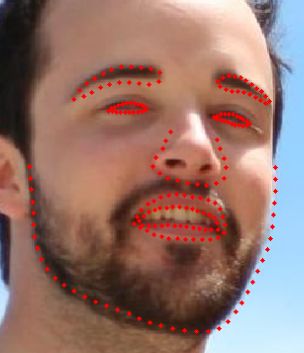
2                                                                                                           Yue Wu, Qiang Ji

                       Table 1: Comparison of the major facial landmark detection algorithms.

               Algorithms                        Appearance            Shape           Performance              Speed
             Holistic Method                     whole face           explicit   poor generalization/good     slow/fast
    Constrained Local Method (CLM)               local patch          explicit             good               slow/fast
       Regression-based Method             local patch/whole face     implicit       good/very good         fast/very fast

eyes can provide the initial guess of the pupil center po-               Facial landmark detection algorithms can be clas-
sitions for eye detection and eye gaze tracking [41]. For           sified into three major categories: the holistic meth-
facial recognition, the landmark locations on 2D image              ods, the Constrained Local Model (CLM) methods, and
are usually combined with 3D head model to “frontal-                regression-based methods, depending on how they model
ize” the face and help reduce the significant within-               the facial appearance and facial shape patterns. The fa-
subject variations to improve recognition accuracy [92].            cial appearance refers to the distinctive pixel intensity
The facial information gained through the facial land-              patterns around the facial landmarks or in the whole
mark locations can provide important information for                face region, while face shape patterns refer to the pat-
human and computer interaction, entertainment, secu-                terns of the face shapes as defined by the landmark loca-
rity surveillance, and medical applications.                        tions and their spatial relationships. As summarized in
    Facial landmark detection algorithms aim to auto-               Table 1, the holistic methods explicitly model the holis-
matically identify the locations of the facial key land-            tic facial appearance and global facial shape patterns.
mark points on facial images or videos. Those key points            CLMs rely on the explicit local facial appearance and
are either the dominant points describing the unique lo-            explicit global facial shape patterns. The regression-
cation of a facial component (e.g., eye corner) or an               based methods use holistic or local appearance infor-
interpolated point connecting those dominant points                 mation and they may embed the global facial shape
around the facial components and facial contour. For-               patterns implicitly for joint landmark detection. In gen-
mally, given a facial image denoted as I, a landmark                eral, the regression-based methods show better perfor-
detection algorithm predicts the locations of D land-               mances recently (details will be discussed later). Note
marks x = {x1 , y1 , x2 , y2 , ..., xD , yD }, where x. and y.      that, some recent methods combine the deep learning
resentment the image coordinates of the facial land-                models and global 3D shape models for detection and
marks.                                                              they are outside the scope of the three major categories.
                                                                    They will be discussed in detail in Section 4.3.
    Facial landmark detection is challenging for sev-
                                                                         The remaining parts of the paper are organized as
eral reasons. First, facial appearance changes signifi-
                                                                    follows. In Sections 2, 3, and 4, we discuss methods in
cantly across subjects under different facial expressions
                                                                    the three major categories: the holistic methods, the
and head poses. Second, the environmental conditions
                                                                    Constrained Local Model methods, and the regression-
such as the illumination would affect the appearance
                                                                    based methods. Section 4.3 is dedicated to the review
of the faces on the facial images. Third, facial occlu-
                                                                    of the recent deep learning based methods. In Section
sion by other objects or self-occlusion due to extreme
                                                                    5, we discus the relationships among methods in the
head poses would lead to incomplete facial appearance
                                                                    three major categories. In Section 6, we discuss the lim-
information.
                                                                    itations of the existing algorithms in “in-the-wild” con-
    Over the past few decades, there have been signifi-             ditions and some advanced algorithms that are specifi-
cant developments of the facial landmark detection al-              cally designed to handle those challenges. In Section 7,
gorithms. The early works focus on the less challenging             we discuss related topics, such as face detection, facial
facial images without the aforementioned facial varia-              landmark tracking, and 3D facial landmark detection.
tions. Later, the facial landmark detection algorithms              In Section 8, we discuss facial landmark annotations,
aim to handle several variations within certain cate-               the popular facial landmark detection databases, soft-
gories, and the facial images are usually collected with            ware, and the evaluation of the leading algorithms. Fi-
“controlled” conditions. For example, in “controlled”               nally, we summarize the paper in Section 9, where we
conditions, the facial poses and facial expressions can             point out future directions.
only be in certain categories. More recently, the research
focuses on the challenging “in-the-wild” conditions, in
which facial images can undergo arbitrary facial expres-            2 Holistic methods
sions, head poses, illumination, facial occlusions, etc. In
general, there is still a lack of a robust method that can              Holistic methods explicitly leverage the holistic fa-
handle all those variations.                                        cial appearance information as well as the global facial
Facial Landmark Detection: a Literature Survey                                                                                        3

shape patterns for facial landmark detection (Figure 2).
In the following, we first introduce the classic holis-
tic method: the Active Appearance Model (AAM) [18].
Then, we introduce its several extensions.
                                                                            Fig. 3: Learned shape variations using AAM model,
                                                                            adapted from [18].

                           Shape
                           model

                                                             Appearance
                                                               model

                                                                            Fig. 4: Learned appearance variations using AAM,
                                                                            adapted from [18].
     Training image                    Shape free textures

                        Fig. 2: Holistic Model.                             Third, to learn the appearance model, image wrap-
                                                                            ping is applied to register the image to the mean shape
                                                                            and generate the shape normalized facial image, de-
                                                                            noted as Ii (W(x0i )), where W(.) indicates the wrap-
                                                                            ping operation. Then, PCA is applied again on the
2.1 Active Appearance Model                                                 shape normalized facial images {Ii (W(x0i ))}Ni=1 to gen-
                                                                            erate a mean appearance A0 and Ka appearance bases
The Active Appearance Model (AAM)1 was introduced                           A = {Am }K   m=1 , as shown in Figure 4. Given the ap-
                                                                                          a

by Taylor and Cootes [27][18]. It is a statistical model                    pearance model A = {Am }K    m=0 , each shape normalized
                                                                                                          a

that fits the facial images with a small number of coeffi-                  facial image can be represented using the appearance
cients, controlling both the facial appearance and shape                    coefficients λ = {λm }Km=1 .
                                                                                                     a

variations. During model construction, AAM builds the
global facial shape model and the holistic facial ap-                                           Ka
                                                                                                X
pearance model sequentially based on Principal Com-                         I(W(x0 )) = A0 +          λm Am                         (2)
                                                                                                m=1
ponent Analysis (PCA). During detection, it identifies
the landmark locations by fitting the learned appear-                       An optional third model may be applied to learn the
ance and shape models to the testing images                                 correlations among the shape coefficients p and appear-
    There are a few steps for AAM to construct the                          ance coefficients λ.
appearance and shape models, given the training facial                          In landmark detection, AAM finds the shape and
images with landmark annotations, denoted as {Ii , xi }N  i=1 ,             appearance coefficients p and λ, as well as the affine
where N is the number of training images. First, Pro-                       transformation parameters {c, θ, tc , tr } that best fit the
crustes Analysis [36] is applied to register all the train-                 testing image, which determine the landmark locations:
ing facial shapes. It removes the affine transformation
(c, θ, tc , tr denote the scale, rotation and translation
                                                                                                Ks
                                                                                                X
parameters) of each face shape xi and generates the
                                                                            x = cR2d (θ)(s0 +         pn ∗ sn ) + t.                (3)
normalized training facial shapes x0i . Second, given the                                       n=1
normalized training facial shapes {x0i }N  i=1 , PCA is ap-
plied to learn the mean shape s0 and a few orthonor-                        Here, R2d (θ) denotes the rotation matrix, and t = {tc , tr }.
mal bases {sn }K    n=1 that capture the shape variations,
                     s                                                      To simplify the notation, in the following the shape co-
where Ks is the number of bases (Figure 3). Given the                       efficients would include both PCA coefficients and affine
learned facial shape bases {sn }K n=0 , a normalized facial
                                    s                                       transformation parameters.
            0                                                                    In general, the fitting procedure can be formulated
shape x can be represented using the shape coefficients
p = {pn }K    n=1 :
               s                                                            by minimizingPthe distance between the reconstructed
                                                                                              Ka
                                                                            images A0 + m=1        λm Am and the shape normalized
              Ks
              X                                                             testing image I(W(p)). The difference is usually re-
x0 = s0 +             pn ∗ sn .                                       (1)   ferred to as the error image, denoted as ∆A:
              n=1
                                                                                                       Ka
                                                                                                       X
 1
   In this paper, we refer Active Appearance Model to the                   ∆A(λ, p) = Diff(A0 +             λm Am , I(W(p)))       (4)
model, independent of the fitting algorithms.                                                          m=1
4                                                                                                      Yue Wu, Qiang Ji

                                                                 Recently, more advanced analytic fitting methods
                                                             only estimate the shape coefficients, which fully deter-
λ∗ , p∗ = arg min ∆A(λ, p)                            (5)    mine the landmark locations as in Equation 3. For ex-
            λ,p
                                                             ample, in [4], the Bayesian Active Appearance Model
In the conventional AAM [27][18], model coefficients         formulates AAM as a probabilistic PCA problem. It
are estimated by iterative calculation of the error im-      treats the texture coefficients as hidden variables and
age based on the current model coefficients and model        marginalizes them out to solve for the shape coeffi-
coefficient update prediction based on the error image.      cients:
                                                                                               Z
                                                             p̃ = arg max lnp(p) = arg max ln p(p|λ)p(λ)dλ. (7)
                                                                     p                  p        λ
2.2 Fitting algorithms
                                                             But exactly integrating out λ can be computationally
Most of the holistic methods focus on improving the          expensive. To alleviate this problem, in [99], Tzimiropou-
fitting algorithms, which involves solving Equation 5.       los and Pantic propose the fast-SIC algorithm and the
They can be classified into the analytic fitting method      fast-forward algorithm. In both algorithms, the appear-
and learning-based fitting method.                           ance coefficient updates ∆λ are represented in terms of
                                                             the shape coefficient updates ∆p, and they are plugged
2.2.1 Analytic fitting methods                               into the nonlinear least square formulation, which is
                                                             then directly minimized to solve for ∆p. Different from
The analytic fitting methods formulate AAM fitting           [4], [99] follows a deterministic approach.
problem as a nonlinear optimization problem and solve
it analytically. In particular, the algorithm searches the   2.2.2 Learning-based fitting methods
best set of shape and appearance coefficients p, λ that
minimize the difference between reconstructed image          Instead of directly solving the fitting problem analyti-
and the testing image with a nonlinear least squares         cally, the learning-based fitting methods learn to pre-
formulation:                                                 dict the shape and appearance coefficients from the im-
                         M
                         X                                   age appearances. They can be further classified into lin-
p̃, λ̃ = arg min kA0 +       λm Am − I(W(p))k22 .     (6)    ear regression fitting methods, nonlinear regression fit-
         p,λ             m                                   ting methods, and other learning-based fitting methods.
             PM                                                  Linear regression fitting methods: The linear
Here, A0 + m λm Am represents the reconstructed face         regression fitting methods assume that there is linear
in the shape normalized frame depending on the shape         relationship between model coefficient updates and the
and appearance coefficients, and the whole objective         error image ∆A(λ, p) or image features I(λ, p). They
function represents the reconstruction error.                learn linear regression function for the prediction, which
    One natural way to solve the optimization problem        follows the conventional AAM as illustrated in the last
is to use the Gaussian-Newton methods. However, since        section.
the Jacobin and Hessian matrix for both p and λ need
                                                                                   Linear Regression
to be calculated for each iteration [48], the fitting pro-   ∆A(λ, p) or I(λ, p) −−−−−−−−−−−−→ ∆λ, ∆p               (8)
cedure is usually very slow. To address this problem,
Baker and Matthews proposed a series of algorithms,          They therefore estimate the model coefficients by iter-
among which the Project Out Inverse Compositional            atively estimating the model coefficient updates, and
algorithm (POIC) [63] and the Simultaneous Inverse           add them to the currently estimated coefficients for
Compositional (SIC) algorithm [7] are two popular            the prediction in the next iteration. For example, in
works. In POIC [63], the errors are projected into space     [26], Canonical Correlation Analysis (CCA) is applied
spanned by the appearance eigenvectors {Am }K    m=1 , and
                                                   a
                                                             to model the correlation between the error image and
its orthogonal complement space. The shape coefficients      the model coefficient updates. It then learns the linear
are firstly searched in the appearance space, and the ap-    regression function to map the canonical projections of
pearance coefficients are then searched in the orthogo-      the error image to the coefficient updates. Similarly, in
nal space, given the shape coefficients. In SIC [7], the     Direct Appearance Model [43], linear model is applied
appearance and shape coefficients are estimated jointly      to directly predict the shape coefficient updates from
with gradient descent algorithm. Compared to POIC,           the principal components of the error images. The lin-
SIC is more computationally intensive, but generalizes       ear regression fitting methods usually differ in the used
better than POIC [38].                                       image features, linear regression models, and whether
Facial Landmark Detection: a Literature Survey                                                                       5

to go to a different feature space to learn the mapping    The learned correlation between shape and appearance
[26] [43].                                                 coefficients can reduce the number of parameters. Such
    Nonlinear regression fitting methods: The lin-         learned correlation may not generalize well to different
ear regression fitting methods assume that the relation-   images. The joint estimation of shape and appearance
ship between features and the error image as shown in      coefficients using Equation 6 can be more accurate. But
Equation 4 around the true solution of model coeffi-       they are more difficult.
cients are close to quadratic, which ensures that an it-
erative procedure with linear updates and adaptive step
size would lead to convergence. However, this linear as-   2.3 Other extensions
sumption is only true when the initialization is around
the true solution which makes the linear regression fit-   2.3.1 Feature representation
ting methods sensitive to the initialization. To tackle
                                                           There are other extensions of the conventional AAM
this problem, the nonlinear regression fitting methods
                                                           methods. One particular direction is to improve the
use nonlinear models to learn the relationship among
                                                           feature representations. It is well known that the AAM
the image features and the model coefficient updates:
                                                           model has limited generalization ability and it has diffi-
                      N onlinear Regression
∆A(λ, p) or I(λ, p) −−−−−−−−−−−−−−−→ ∆λ, ∆p          (9)   culty fitting the unseen face variations (e.g. across sub-
                                                           jects, illumination, partial occlusion, etc.) [37][38]. This
For example, in [83], boosting algorithm is proposed       limitation is partially due to the usage of raw pixel in-
to predict the coefficient updates from the appearance.    tensity as features. To tackle this problem, some algo-
It combines a set of weak learners to form a strong        rithms use more robust image features. For example,
regressor, and the weak learners are developed based       in [45], instead of using the raw pixel intensity, the
on the Haar-like features and the one-dimensional de-      wavelet features are used to model the facial appear-
cision stump. The strong nonlinear regressor can be        ance. In addition, only the local appearance information
considered as an additive piecewise function. In [95],     is used to improve the robustness to partial occlusion
Tresadern et al. compared the linear and nonlinear re-     and illumination. In [47], Gabor wavelet with Gaussian
gression algorithms. The used nonlinear regression al-     Mixture model is used to model the local image ap-
gorithms include the additive piecewise function devel-    pearance, which enables fast local point search. Both
oped with boosting algorithm in [83] and the Relevance     methods improve the performances of the conventional
Vector Machine [104]. They empirically showed that         AAM method.
nonlinear regression method is better at the first few
iterations to avoid the local minima, while linear re-     2.3.2 Ensemble of AAM models
gression is better when the estimation is close to the
true solution.                                             A single AAM model inherently assumes linearity in
                                                           face shape and appearance variation. Realizing this lim-
2.2.3 Discussion: analytic fitting methods vs.             itation, some methods utilize ensemble models to im-
learning-based fitting methods                             prove the performance. For example, in [71], sequential
                                                           regression AAM model is proposed, which trains a seri-
Compared to the analytic fitting methods solved with       als of AAMs for sequential model fitting in a cascaded
gradient descent algorithm with explicit calculation of    manner. AAM in the early stage takes into account of
the Hessian and Jacobian matrices, the learning-based      the large variations (e.g. pose), while those in the later
fitting methods use constant linear or nonlinear regres-   stage fits to the small variations. In this work, both
sion functions to approximate the steepest descent di-     independent ensemble AAMs and coupled sequential
rection. As a result, the learning-based fitting methods   AAMs are used. The independent ensemble AAMs use
are generally fast but they may not be accurate. The       independently perturbed model coefficients with differ-
analytic methods do not need training images, while the    ent settings, while the coupled ensemble AAMs apply
fitting methods do. The learning-based fitting methods     the learned prediction model in the first few levels to
usually use a third PCA to learn the joint correlations    generate the perturbed training data in the later level.
among the shape and appearance coefficients and fur-       Both boosting regression and random forest regressions
ther reduce the number of unknown coefficients, while      are utilized predict the model updates. Similar to the
the analytic fitting methods usually do not. But, for      coupled ensemble AAMs in [71], in [82], AAM fitting
the analytic fitting methods, the interaction among ap-    problem is formulated as an optimization problem with
pearance and shape coefficients can be embedded in         stochastic gradient descent solution. It leads to an ap-
the joint fitting objective function as in Equation 6.     proximated algorithm that iteratively learns the linear
6                                                                                                                                          Yue Wu, Qiang Ji

                                                                                            Here, each landmark location xd is determined by p as
                                                                                            in Equation 3.
                                                                                                In the probabilistic view point, CLM can be inter-
                                                                                            preted as maximizing the product of the prior proba-
Facial image        Local appearance model   Global face shape model
                    detect each landmark     captures the face shape
                                                                        Facial landmark
                                                                        detection results
                                                                                            bility of the facial shape patterns p(x; η) of all points
                    independently            variations to refine the                       and the local appearance likelihoods p(xd |I; θd ) of each
                                             local detection results
                                                                                            point:
                   Fig. 5: Constrained Local Method.                                                               D
                                                                                                                   Y
                                                                                            x̃ = arg max p(x; η)         p(xd |I; θd )                (12)
                                                                                                    x
                                                                                                                   d=1
prediction model from the training data with perturbed
model coefficients at the first iteration, and then up-                                     Similar to the deterministic formulation, the prior can
dates the model coefficients for training data to be used                                   also be applied to the shape coefficients p, and Equa-
in the next iteration following a cascaded manner. Dif-                                     tion 12 becomes:
ferent from [71], [82] uses different subsets of training                                                            D
                                                                                                                     Y
data in different stages to escape from the local minima.                                   p̃ = arg max p(p; ηp )         p(xd (p)|I; θd ).          (13)
                                                                                                    p
                                                                                                                     d=1

3 Constrained local methods                                                                     For both the deterministic and the probabilistic CLMs,
                                                                                            there are two major components. The first component
As shown in Figure 5, the Constrained Local Model                                           is the local appearance model embedded in Dd (xd , I) or
(CLM) methods [24][84] infer the landmark locations x                                       p(xd |I; θd ) in Equations 10, 11, 12, and 13. The second
based on the global facial shape patterns as well as the                                    component refers to the facial shape pattern constraints
independent local appearance information around each                                        either applied to the shape model coefficients p or the
landmark, which is easier to capture and more robust                                        shape x itself, as penalty terms or probabilistic prior
to illumination and occlusion, comparing to the holistic                                    distributions. The two components are usually learned
appearance.                                                                                 separately during training and they are combined to
                                                                                            infer landmark locations during landmark detection. In
                                                                                            the following, we will discuss each component, and how
3.1 Problem formulation                                                                     to combine them for landmark detection.

In general, CLM can be formulated either as a deter-
ministic or probabilistic method. In the deterministic                                      3.2 Local appearance model
view point, CLM [24][84] finds the landmarks by min-
imizing the misalignment errors subject to the shape                                        The local appearance model assigns confidence score
patterns:                                                                                   Dd (xd , I) or probability p(xd |I; θd ) that the landmark
                                                                                            with index d is located at a specific pixel location xd
                                 D
                                 X                                                          based on the local appearance information around xd
x̃ = arg min Q(x) +                    Dd (xd , I)                                 (10)
               x                                                                            of image I. The local appearance models can be cate-
                                 d=1
                                                                                            gorized into classifier-based local appearance model and
Here, xd represents the positions of different landmarks                                    the regression-based local appearance model.
in x. Dd (xd , I) represents the local confidence score
around xd . Q(x) represents a regularization term to                                        3.2.1 Classifier-based local appearance model
penalize the infeasible or anti-anthropology face shapes
in a global sense. The intuition is that we want to find                                    The classifier-based local appearance model trains bi-
the best set of landmark locations that have strong in-                                     nary classifier to distinguish the positive patches that
dependent local support for each landmark and satisfy                                       are centered at the ground truth locations and the neg-
the global shape constraint.                                                                ative patches that are far away from the ground truth
    The shape regularization can be applied to the shape                                    locations. During detection, the classifier can be applied
coefficients p. If we denote the regularization term as                                     to different pixel locations to generate the confidence
Qp (p), Equation 10 becomes:                                                                scores Dd (xd , I) or probabilities p(xd |I; θd ) through vot-
                                   D
                                                                                            ing. Different image features and classifiers are used.
                                   X
p̃ = arg min Qp (p) +                    Dd (xd (p), I)                            (11)     For example, in the original CLM work [24] and FPLL
               p
                                   d=1
                                                                                            [125], template based method is used to construct the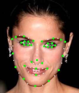
Facial Landmark Detection: a Literature Survey                                                                         7

classifier. The original CLM uses the raw image patch,
while FPLL uses the HOG feature descriptor. In [11][10],
SIFT feature descriptor and SVM classifier are used to
learn the appearance model. In [22], Gentle Boost clas-
sifier is used. One issue with the classifier-based local
appearance model is that it is unclear which feature
representation and classifier to use. Even though SIFT      Fig. 6: Regression-based local appearance model [19].
and HOG features and SVM classifier are the popular
choice, there is some work[105] that learns the features
using the deep learning methods, and it is shown that       For example, a large local patch is more robust, while
the learned features are comparable to HOG and SIFT.        it is less accurate for precise landmark localization. A
                                                            small patch with more distinctive appearance informa-
3.2.2 Regression-based local appearance model               tion would lead to more accurate detection results. To
                                                            tackle this problem, some algorithms [76] combine the
During training, the goal of the regression-based local     large patch and small patch for estimation and adapt
appearance model is to predict the displacement vector      the sizes of the patches or searching regions across it-
∆x∗d = x∗d − x, which is the difference between any pixel   erations.
location x and the ground truth landmark location x∗d           Second, it is unclear which approach to follow, among
from the local appearance information around x using        the classifier-based methods and the regression-based
the regression models. During detection, the regression     methods. One advantage of the regression-based ap-
model can be applied to patches at different locations      proach is that it only needs to calculate the features
x in a region of interest to predict ∆xd , which can be     and predict the displacement vectors for a few sample
added to the current location to calculate xd .             patches in testing. It is more efficient than the classifier-
                                                            based approach that scans all the pixel locations in the
Regression : I(x) → ∆xd                             (14)    region of interest. It is empirically shown in [22] that
                                                            the Gentleboost regressor as a regression-based appear-
                                                            ance model is better than the Gentleboost classifier as
xd = x + ∆xd ;                                      (15)    a classifier-based local appearance model.

Predictions from multiple patches can be merged to
calculate the final prediction of the confidence score      3.3 Face shape models
or probability through voting (Figure 6). Different im-
age features and regression models are used. In [22],       The face shape model captures the spatial relationships
Cristinacce and Cootes proposed to use the Gentleboost      among facial landmarks, which constrain and refine the
as the regression function. In Cootes’s later work [19],    landmark location search. In general, they can be clas-
he extended the method and used the random forests          sified into deterministic face shape models and proba-
as the regressor, which shows better performance. In        bilistic face shape models.
[102], Adaboost feature selection method is combined
with SVM regressor to learn the regression function. In     3.3.1 Deterministic face shape models
[88], nonparametric appearance model is used for loca-
tion voting based on the contextual features around the     The deterministic face shape models utilize determinis-
landmark. Similar to the classifier-based methods, it’s     tic models to capture the face shape patterns. They as-
unclear which feature and regression function to use.       sign low fitting errors to the feasible face shapes and pe-
It is empirically shown in [61] that the LBP features       nalize infeasible face shapes. For example, Active shape
are better than the Haar features and LPQ descriptor.       model (ASM) [20] is the most popular and conventional
Another issue is that since the regression-based local      face shape model. It learns the linear subspaces of the
appearance model performs one-step prediction. The          training face shapes using Principal Component Anal-
prediction may not be accurate if the current positions     ysis as in Equation 1. The face can be evaluated by
are far away from the true target.                          the fitness to the subspaces. It has been used both
                                                            in the holistic AAM method and the CLM methods.
3.2.3 Discussion: local appearance model                    Since one linear ASM may not be effective to model
                                                            the global face shape variations, in [54], two levels of
There are several issues related to the local appearance    ASMs are constructed. One level of ASMs are used to
model. First, there exists accuracy-robustness tradeoffs.   capture the shape patterns of each facial component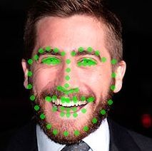
8                                                                                                        Yue Wu, Qiang Ji

independently, and the other level of ASM is used for         Algorithm 1: Iterative methods
modeling the joint spatial relationships among facial             Data: The initial searching regions
components. In [125], Zhu and Ramanan built pose-                                   (1)   (1)      (1)
                                                                         Ω (1) = {Ω1 , Ω2 , ..., ΩD } for all D
dependent tree structure face shape model to capture                     landmarks.
the local nonlinear shape patterns, in which each land-           Result: The detected landmark locations x or the
                                                                           shape coefficients p that determine the
mark is represented as a tree node. Improving upon                         landmark locations.
[125], the method in [44] builds two levels of tree struc-    1   for t=1 until convergence do
                                                                                                      (t)
tured models focusing on different numbers of landmark        2       Within the searching region Ωd , detect each
points on images with different resolutions. In [9], in-              facial landmark point independently using the
stead of using the 2D facial shape models, Baltrusaitis               local appearance models, and treat them as the
                                                                      measurements mt .
et al. proposed to embed the facial shape patterns into       3       Refine the measurements m jointly with the face
a 3D facial deformable model to handle pose variations.               shape model constraint, and output the estimated
During detection, both the 3D model coefficients and                  locations xt or shape coefficients pt .
                                                                                                        (t+1)
the head pose parameters are jointly estimated for land-      4       Modify each searching region Ωd         to be around
                                                                      currently estimated landmark location.
mark detection. This method, however, requires to learn
3D deformable model, and to estimate head pose. 3D
landmark detection will be further discussed in Section
7.3.                                                         will be discussed in Section 6 ). In addition, it’s time-
                                                             consuming to generate the facial landmark annotations
3.3.2 Probabilistic face shape models                        under different facial shape variations, and more com-
                                                             plex model requires more data to train. For example,
The probabilistic face shape models capture the facial       due to facial occlusion, complete landmark annotation
shape patterns in a probabilistic manner. They assign        is infeasible on the self-occluded profile faces.
high probabilities to face shapes that satisfy the anthro-
pological constraint learned from training data and low
probabilities to other infeasible face shapes. The early     3.4 Landmark point detection via optimization
probabilistic face shape model is the switching model
proposed in [94]. It can automatically switch the states     Given the local appearance models and the face shape
of facial components (e.g. mouth open and close) to          models described above, CLMs combine them for de-
handle different facial expressions. In [102][61], a gen-    tection using Equations 10, 11, 12 or 12. This is a
erative Boosted Regression and graph Models based            non-trivial task, since the analytic representation of
method (BoRMaN) constructed based on the Markov              the local appearance model is usually not directly com-
Random Field is proposed. Each node in the MRF cor-          putable from the local appearance model and the whole
responds to the relative positions of three points, and      objective function is usually non-convex. To solve this
the MRF as a whole can model the joint relationships         problem, there are two sets of approaches, including the
among all landmarks. In [11][10], Belhumeur et al. pro-      iterative methods and the joint optimization methods.
posed a non-parametric probabilistic face shape model
with optimization strategy to fit the facial images. In      3.4.1 Iterative methods
[108][105], Wu and Ji proposed a discriminative deep
face shape model based on the Restricted Boltzmann           The iterative methods decompose the optimization prob-
Machine model. It explicitly handles face pose and ex-       lem into two steps: landmark detection by local ap-
pression variation, by decoupling the face shapes into       pearance model and location refinement by the shape
head pose related part and expression related part. Com-     model. They occur alternately until the estimation con-
pared to the other probabilistic face shape models, it       verges. Specifically, it estimates the optimal landmark
can better handle facial expressions and poses within a      positions that best fit the local appearance models for
unified model.                                               each landmark in the local region independently, and
                                                             then refines them jointly with the face shape model.
3.3.3 Discussion: face shape model                           The detailed algorithm is shown in Algorithm 1. There
                                                             are a few algorithms [24][22][19][102][61][108][109] that
Despite of the recent developments of the face shape         follow the iterative framework. Those methods differ in
model, its construction is still an unsolved problem.        the used local appearance models and facial shape mod-
There is a lack of a unified shape model that can cap-       els, and we have discussed their particular techniques
ture all natural facial shape variations (some methods       in the above sections.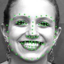
Facial Landmark Detection: a Literature Survey                                                                         9

3.4.2 Joint optimization methods                                4 Regression-based methods

Different from the iterative methods, the joint optimiza-       The regression-based methods directly learn the map-
tion methods aim to perform joint inference. The chal-          ping from image appearance to the landmark locations.
lenge is that they have to find a way to represent the          Different from the Holistic Methods and Constrained
detection results from independent local point detec-           Local Model methods, they usually do not explicitly
tors and combine them with the face shape model for             build any global face shape model. Instead, the face
joint inference. To tackle this problem, in [84], the inde-     shape constraints may be implicitly embedded. In gen-
pendent detection results are represented with Kernel           eral, the regression-based methods can be classified into
Dense Estimation (KDE) and the optimization problem             direct regression methods, cascaded regression methods,
is solved with EM algorithm subject to the shape con-           and deep-learning based regression methods. Direct re-
straint, which treats the true landmark location as hid-        gression methods predict the landmarks in one iteration
den variables. It also discusses some other methods to          without any initialization, while the cascaded regression
represent the local detection results, such as using the        methods perform cascaded prediction and they usually
Isotropic Gaussian Model [20], the Anisotropic Gaus-            require initial landmark locations. The deep-learning
sian model [67], and Gaussian Mixture Model [40]. In            based methods follow either the direct regression or the
the Consensus of exemplars work [11][10], in a Bayesian         cascaded regression. Since they use unique deep learn-
formulation, the local detector is combined with the            ing methods, we discuss them separately.
nonparametric global model. Because of the special prob-
abilistic formulation, the objective function can be opti-
mized in a “brutal-force” way with RANSAC strategy.
                                                                4.1 Direct regression methods
    There are also algorithms that simplify the shape
model to use efficient inference methods. For example,
                                                                The direct regression methods learn the direct mapping
in [125], due to the usage of simple tree structure face
                                                                from the image appearance to the facial landmark loca-
shape model, dynamic programming can be applied to
                                                                tions without any initialization of landmark locations.
solve the optimization problem efficiently. In [23], by
                                                                They are typically carried out in one step. They can
converting the objective function into a linear program-
                                                                be further classified into local approaches and global ap-
ming problem, Nelder-Meade simplex method is applied
                                                                proaches. The local approaches use image patches, while
to solve the optimization problem.
                                                                the global approaches use the holistic facial appearance.
                                                                    Local approaches: The local approaches sample
3.4.3 Discussion: optimization                                  different patches from the face region, and build struc-
                                                                tured regression models to predict the displacement
The iterative methods and joint optimization meth-              vectors (target face shape to the locations of the ex-
ods have their own benefits and disadvantages. On one           tracted patches), which can be added to the current
hand, the iterative methods are generally more efficient,       patch location to produce all landmark locations jointly.
but it may fail into the local minima due to the itera-         The final facial landmark locations can be calculated by
tive procedure. On the other hand, the joint optimiza-          merging the prediction results from multiple sampled
tion methods are usually more difficult to solve and are        patches. Note that, this is different from the regression-
computationally expensive.                                      based local appearance model that predicts each point
     Note that, as shown in Equations 10, 11, 12 or 12,         independently (Section 3.2.2), while the local approaches
in CLM, we would either infer the exact landmark lo-            here predict the updates for all points simultaneously.
cations x or the shape coefficients that can fully deter-       For example, in [25], conditional Regression Forests are
mine the landmark locations (e.g. shape coefficients p          used to learn the mapping from randomly sampled patches
when using ASM as the face shape model as in Equa-              in the face region to the face shape updates. In ad-
tion 3). There is a dilemma. On one hand, since small           dition, several head pose dependent models are built
shape model errors may lead to large landmark detec-            and they are combined together for detection. Simi-
tion errors, directly predicting the landmark locations         larly, privileged Information-based conditional random
may be a better choice. On the other hand, it may be            forests model [113] uses additional facial attributes (e.g.
easier to design the cost function for the model coeffi-        head pose, gender, etc.) to train regression forests to
cients than the shapes. For example, in ASM [20], it is         predict the face shape updates. Different from [25] which
relatively easier to set up the range for the model coef-       merges the prediction from different pose-dependent
ficients while it is difficult to directly set the constraint   models, in testing, it predicts the attributes first and
for the face shapes.                                            then performs attribute dependent landmark location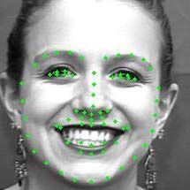
10                                                                                                    Yue Wu, Qiang Ji

 Algorithm 2: Cascaded regression detection
 1   Initialize the landmark locations x0 (e.g. mean face).
 2   for t=1, 2, ..., T or convergence do
 3       Update the landmark locations, given the image
         and the current landmark location.
                                                                  Iteration 1        Iteration 2           Iteration t
        ft : I, xt−1 → ∆xt

        xt = xt−1 + ∆xt                                                   Fig. 7: Cascaded regression methods.
                                                 T
 4   Output the estimated landmark locations x       .

                                                                  Different shape-indexed image appearance and re-
                                                              gression models are used. For example, in [14], Cao et
estimation. In this case, the landmark prediction accu-       al. proposed the shape-indexed pixel intensity features
racy will be affected by attribute prediction. One issue      which are the pixel intensity differences between pairs of
with the local regression methods is that the indepen-        pixels whose locations are defined by their relative po-
dent local patches may not convey enough information          sitions to the current shape. In [76], Ren et al. proposed
for global shape estimation. In addition, for images with     to learn discriminative binary features by the regression
occlusion, the randomly sampled patches may lead to           forests for each landmark independently. Then, the bi-
bad estimations.                                              nary features from all landmarks are concatenated and
    Global approaches: The global approaches learn            a linear regression function is used to learn the joint
the mapping from the global facial image to landmark          mapping from appearance to the global shape updates.
locations directly. Different from the local approaches,      In [52], ensemble of regression trees are used as regres-
the holistic face conveys more information for landmark       sion models for face alignment. By modifying the ob-
detection. But, the mapping from the global facial ap-        jective function, the algorithm can use training images
pearance to the landmark locations is more difficult to       with partially labeled facial landmark locations.
learn, since the global facial appearance has significant         Among different cascaded regression methods, the
variations, and they are more susceptible to facial occlu-    Supervised Descent Method (SDM) in [110] achieves
sion. The leading approaches [91][119] all use the deep       promising performances. It formulates face alignment
learning methods to learn the mapping, which we will          as a nonlinear least squares problem. In particular, as-
discuss in details in Section 4.3. Note that, since the       suming the appearance features (e.g. SIFT) of the local
global approaches directly predict landmark locations,        patches around the true landmark locations x∗ are de-
they are different from the holistic methods in Section       noted as Φ(I(x∗ )), the goal of landmark detection is to
2 that construct the shape and appearance models and          estimate the location updates δx starting from an ini-
predict the model coefficients.                               tial shape x0 , so that the feature distance is minimized:

                                                              δx̃ = arg min f (x0 + δx)
4.2 Cascaded regression methods                                           δx
                                                                                                                         (16)
                                                                 = arg min kΦ(I(x∗ )) − Φ(I(x0 + δx))k22
In contrast to the direct regression methods that per-                    δx

form one-step prediction, the cascaded regression meth-       By applying the second order Taylor expansion with
ods start from an initial guess of the facial landmark lo-    Newton-type method, the shape updates are calculated:
cations (e.g. mean face), and they gradually update the
landmark locations across stages with different regres-
                                                                                                1
sion functions learned for different stages (Figure 7).       f (x0 +δx) ≈ f (x0 )+Jf (x0 )T δx− δxT Hf (x0 )δx (17)
                                                                                                2
Specifically, in training, in each stage, regression mod-
els are applied to learn the mapping between shape-
indexed image appearances (e.g., local appearance ex-         δx = −Hf (x0 )−1 Jf (x0 )
tracted based on the currently estimated landmark lo-                                                                    (18)
                                                                 = −2Hf (x0 )−1 JTΦ (Φ(I(x0 )) − Φ(I(x∗ )))
cations) to the shape updates. The learned model from
the early stage will be used to update the training data      To directly calculate δx analytically is difficult, since
for the training in the next stage. During testing, the       it requires the calculation of the Jacobin and Hessian
learned regression models are sequentially applied to         matrix for different x0 . Therefore, supervised descent
update the shapes across iterations. Algorithm 2 sum-         method is proposed to learn the descent direction with
marizes the detection process.                                regression method. It is then simplified as the cascaded
Facial Landmark Detection: a Literature Survey 11
regression method with linear regression function, which
can predict the landmark location updates from shape-
indexed local appearance.
R = −2Hf (x0 )−1 JTΦ (19)
b ≈ 2Hf (x0 )−1 JTΦ Φ(I(x∗ )) (20) Fig. 8: CNN model structure, adapted from [91].
minima while the iteration continues. It is also possi-
δx = RΦ(I(x0 )) + b (21)
ble that the prediction is already close to the optimum
The regression functions are different for different iter- after a few stages. In the existing methods [76], it is
ations, but they ignore different possible starting shape only shown that the cascaded regression methods can
x0 within one iteration. improve the performance over different cascaded stages,
There are some other variations of the cascaded re- but it doesn’t know when to stop.
gression methods. For example, in [6], instead of learn-
ing the regression functions in a cascaded manner (the
later level depends on the former level), a parallel learn- 4.3 Deep learning based methods
ing method is proposed, so that the later level only
needs the statistic information from the previous level. Recently, deep learning methods become popular tools
Based on the parallel learning framework, it’s possi- for computer vision problems. For facial landmark de-
ble to incrementally update the model parameters in tection and tracking, there is a trend to shift from tradi-
each level by adding a few more training samples, which tional methods to deep learning based methods. In the
achieves fast training. early work [108], the deep boltzmann machine model,
The cascaded regression methods are more effective which is a probabilistic deep model, was used to capture
than the direct regression since they follow the coarse- the facial shape variations due to poses and expressions
to-fine strategy. The regression functions in the early for facial landmark detection and tracking. More re-
stage can focus on the large variations while the regres- cently, the Convolutional Neural Network (CNN) mod-
sion functions in the later stage may focus on the fine els become the dominate deep learning models for fa-
search. cial landmark detections, and most of them follow the
However, for cascaded regression methods, it is un- global direct regression framework or cascaded regres-
clear how to generate the initial landmark locations. sion framework. Those methods can be broadly clas-
The popular choice is to use the mean face, which may sified into pure-learning methods and hybrid methods.
be sub-optimal for images with large head poses. To The pure-learning methods directly predict the facial
tackle this problem, there are some hybrid methods landmark locations, while the hybrid methods combine
that use the direct regression methods to generate the deep learning methods with computer vision projection
initial estimation for cascaded regression methods. For model for prediction.
example, in [118], a model based on auto-encoder is Pure-learning methods: Methods in this cate-
proposed. It first performs direct regression on down- gory use the powerful CNN models to directly predict
sampled lower-resolution images, and then refine the the landmark locations from facial images. [91] is the
prediction in a cascaded manner with higher resolution early work and it predicts five facial key points in a cas-
images. In [123], a coarse to fine searching strategy is caded manner. In the first level, it applies a CNN model
employed and the initial face shape is continuously up- with four convolution layers (Figure 8) to predict the
dated based on the estimation from last stage. There- landmark locations given the facial image determined
fore, a more close-to-solution initialization will be gen- by the face bounding box. Then, several shallow net-
erated and fine facial landmark detection results are works refine each individual point locally.
easier to get. Ever since then, there are several improvements over
Another issue about the cascaded regression method [91] in two directions. In the first direction, [119][120]
is that the algorithms apply a fixed number of cascaded and [75] leverage multi-task learning idea to improve
prediction, and there is no way to judge the quality of the performance. The intuition is that multiple tasks
landmark prediction and adapt the necessary cascaded could share the same representation and their joint re-
stages for different testing images. In this case, it is pos- lationships would improve the performances of individ-
sible that the prediction is already trapped in a local ual tasks. For example, in [119][120], multi-task learning12 Yue Wu, Qiang Ji
is combined with CNN model to jointly predict facial
landmarks, facial head pose, facial attributes etc. A sim-
ilar multi-task CNN framework is proposed in [75] to
jointly perform face detection, landmark localization,
pose estimation, and gender recognition. Different from
[119] [120], it combines features from multiple convolu-
tional layers to leverage both the coarse and fine feature
representations.
In the second direction, some works improve the cas-
Fig. 9: 3D face model and its projection based on the
caded procedure of method [91]. For example, in [122],
head pose parameters (i.e. pitch, yaw, roll angles)
similar cascaded CNN model is constructed to predict
many more points (68 landmarks instead of 5). It starts
from the prediction of all 68 points and gradually de- Table 2 2 summarizes the CNN structures of the
couples the prediction into local facial components. In leading methods. We list their numbers of convolutional
[118], the deep auto-encoder model is used to perform layers, the numbers of fully connected layer, whether a
the same cascaded landmark search. In [96], instead of 3D model is used, and whether the cascaded method
training multiple networks in a cascaded manner, Trige- is used. For the cascaded methods, if different model
orgis et. al trained a deep convolutional Recurrent Neu- structures are used for different layers, we only list the
ral Network (RNN) for end-to-end facial landmark de- model in the first level. As can be seen, the models
tection to mimic the cascaded behavior. The cascaded proposed for facial landmark detection usually contain
stage is embedded into the different time slices of RNN. around four convolutional layers and one fully connected
layer. The model complexity is on par with the deep
Hybrid deep methods: The hybrid deep methods models used for other related face analysis tasks, such
combine the CNN with 3D vision, such as the projec- as head pose estimation [70], age and gender estimation
tion model and 3D deformable shape model (Figure 9). [55], and facial expression recognition [58], which usu-
Instead of directly predicting the 2D facial landmark ally have similar or smaller numbers of convolutional
locations, they predict 3D shape deformable model co- layers. For the face recognition problem, the CNN mod-
efficients and the head poses. Then, the 2D landmark els are usually more complex with more convolutional
locations can be determined through the computer vi- layers (e.g. eight layers) and fully connected layers [90]
sion projection model. For example, in [124], a dense [85] [92]. It is in part due to the fact that there is much
3D face shape model is construct. Then, an iterative more training data (e.g., 10M+, 100M+ images) for
cascaded regression framework and deep CNN models face recognition comparing to the data set used for
are used to update the coefficients of 3D face shape facial landmark detections (e.g., 20K+ images) [75].
and pose parameters. In each iteration, to incorporate It is still an open question whether adding more data
the currently estimated 3D parameters, the 3D shape is would improve the performances of facial landmark de-
projected to 2D using the vision projection model and tection. Another promising direction is to leverage the
the 2D shape is used as additional input of the CNN multi-task learning idea to jointly predict related tasks
model for regression prediction. Similarly, in [50], in a (e.g., landmark detection, pose, age and gender) with
cascaded manner, the whole facial appearance is used in a deeper model to boost the performances for all tasks
the first cascaded CNN model to predict the updates of [75].
3D shape parameters and pose, while the local patches
are used in the later cascaded CNN models to refine the
landmarks. 4.4 Discussion: regression-based methods
Compared to the pure-learning methods, the 3D Among different regression methods, cascaded regres-
shape deformable model and pose parameters of the sion method achieves better results than direct regres-
hybrid methods are more compact ways to represent sion. Cascaded regression with deep learning can fur-
the 2D landmark locations. Therefore, there are fewer ther improve the performance. One issue for the regression-
parameters to estimate in CNN and shape constraint based methods is that since they learn the mapping
can be explicitly embedded in the prediction. Further- from the facial appearance within the face bounding
more, due to the introduction of 3D pose parameters, 2
For [75], we list the landmark prediction model instead of
they can better handle pose variations. the multi-task prediction model for fair comparison.Facial Landmark Detection: a Literature Survey 13
Table 2: CNN model structures of the leading methods.
methods # convolutional layer # fully connected layer, # features 3D model cascaded method
Sun et. al [91] 4 1 (120) N Y
Zhang et. al [119] 4 1 (100) N N
Ranjan et. al [75] 5 + Dim. reduction 1 (3072) N N
Zhou et. al [122] 4 1 (120) N Y
Zhu et. al [124] 4 2 (256, 234) Y Y
Jourabloo and Liu [50] 3 1 (150) Y Y
box region to the landmarks, they may be sensitive predict the landmarks directly by fitting the local ap-
to the used face detector and the quality of the face pearances without explicit 2D shape model. The fitting
bounding box. Because the size and location of the ini- problem of holistic methods can be solved with learn-
tial face is determined by the face bounding box, al- based approaches or analytically as discussed in section
gorithms trained with one face detector may not work 2.2, while all the cascaded regression methods perform
well if a different biased face detector is used in testing. estimation by learning. While the learning-based fit-
This issue has been studied in [78]. ting methods for holistic models usually use the same
Even though we mentioned that the regression-based model for coefficient updates in an iterative manner,
methods do not explicitly build the facial shape model, the cascaded regression methods learn different regres-
the facial shape patterns are usually implicitly embed- sion models in a cascaded manner. The AAM model
ded. In particular, since the regression-based methods [82] discussed in section 2.3.2 as one particular type of
predict all the facial landmark locations jointly, the holistic method is very similar to the Supervised De-
structured information as well as the shape constraint scent Methods (SDM) [110] as one particular type of
are implicitly learned through the process. the cascaded regression method. Both train cascaded
models to learn the mapping from shape-indexed fea-
tures to shape (coefficient) updates. The trained model
5 Discussions: relationships among methods in in the current cascaded stage will modify the training
three major categories. data to train the regression model in the next state.
While the former holistic method fits the holistic ap-
In the previous three sections, we discussed the facial pearance and predicts the model coefficients, SDM fits
landmark detection methods in three major categories: the local appearance and predicts the landmark loca-
the holistic methods, the Constrained Local Methods tions.
(CLM), and the regression-based methods as summa- Third, there are similarities among the regression-
rized in Figure 10. There exist similarities and relation- based local appearance model used in CLM in section
ships among the three major approaches. 3.2.2 and the regression-based methods in section 4.
First, both the holistic methods and CLMs would Both of them predict the location updates from an ini-
capture the global facial shape patterns using the ex- tial guess of the landmark locations. The former ap-
plicitly constructed facial shape models, which are usu- proach predicts each landmark location independently,
ally shared between them. CLMs improve over the holis- while the later approach predicts them jointly, so that
tic methods in that they use the local appearance around shape constraint can be embedded implicitly. The for-
landmarks instead of the holistic facial appearance. The mer approach usually performs one-step prediction with
motivation is that it’s more difficult to model the holis- the same regression model, while the later approach can
tic facial appearances, and the local image patches are apply different regression functions in a cascaded man-
more robust to illumination changes and facial occlu- ner.
sion compared to the holistic appearance models. Fourth, compared to the holistic methods and con-
Second, the regression-based methods, especially for strained local methods, the regression-based methods
the cascaded regression methods [110] share similar in- may be more promising. The regression-based methods
tuitions as the holistic AAM [7][82]. For example, both bypass the explicit face shape modeling and embed the
of them estimate the landmarks by fitting the appear- face shape pattern constraint implicitly. The regression-
ance and they all can be formulated as a nonlinear least based methods directly predict the landmarks, instead
squares problem as shown in Equation 6 and 16. How- of the model coefficients as in the holistic methods and
ever, the holistic methods predict the 2D shape and some CLMs. Directly predicting the shape usually can
appearance model coefficients by fitting the holistic ap- achieve better accuracy since small model coefficient
pearance model, while the cascaded regression methods errors may lead to large landmark errors.You can also read


