Shape Google: Geometric Words and Expressions for Invariant Shape Retrieval
←
→
Page content transcription
If your browser does not render page correctly, please read the page content below
1
Shape Google: Geometric Words and Expressions for Invariant
Shape Retrieval
ALEXANDER M. BRONSTEIN
Tel-Aviv University
MICHAEL M. BRONSTEIN
Università della Svizzera Italiana
and
LEONIDAS J. GUIBAS and MAKS OVSJANIKOV
Stanford University
The computer vision and pattern recognition communities have recently witnessed a surge of feature-based methods in object recognition and image retrieval
applications. These methods allow representing images as collections of “visual words” and treat them using text search approaches following the “bag of
features” paradigm. In this article, we explore analogous approaches in the 3D world applied to the problem of nonrigid shape retrieval in large databases.
Using multiscale diffusion heat kernels as “geometric words,” we construct compact and informative shape descriptors by means of the “bag of features”
approach. We also show that considering pairs of “geometric words” (“geometric expressions”) allows creating spatially sensitive bags of features with better
discriminative power. Finally, adopting metric learning approaches, we show that shapes can be efficiently represented as binary codes. Our approach achieves
state-of-the-art results on the SHREC 2010 large-scale shape retrieval benchmark.
Categories and Subject Descriptors: H.3.3 [Information Storage and Retrieval]: Information Search and Retrieval—Retrieval models; selection process; I.2.10
[Computing Methodologies]: Vision and Scene Understanding—Shape; I.3.5 [Computer Graphics]: Computational Geometry and Object Modeling—Curve,
surface, solid, and object representations; geometric algorithms, languages, and systems; object hierarchies; I.3.7 [Computer Graphics]: Three-Dimensional
Graphics and Realism; I.3.8 [Computer Graphics]: Applications
General Terms: Algorithms, Design, Performance
ACM Reference Format:
Bronstein, A. M., Bronstein, M. M., Guibas, L. J., and Ovsjanikov, M. 2011. Shape Google: Geometric words and expressions for invariant shape retrieval.
ACM Trans. Graph. 30, 1, Article 1 (January 2011), 20 pages. DOI = 10.1145/1899404.1899405 http://doi.acm.org/10.1145/1899404.1899405
1. INTRODUCTION rich variability, and shape retrieval must often be invariant under
different classes of transformations. A particularly challenging set-
The availability of large public-domain databases of 3D models ting, which we address in this article, is the case of nonrigid or
such as the Google 3D Warehouse has created the demand for deformable shapes, which includes a wide range of shape transfor-
shape search and retrieval algorithms capable of finding similar mations such as bending and articulated motion.
shapes in the same way a search engine responds to text queries. An analogous problem in the image domain is image retrieval:
However, while text search methods are sufficiently developed to the problem of finding images depicting similar scenes or objects.
be ubiquitously used, for example, in a Web application, the search Similar to 3D shapes, images may manifest significant variabil-
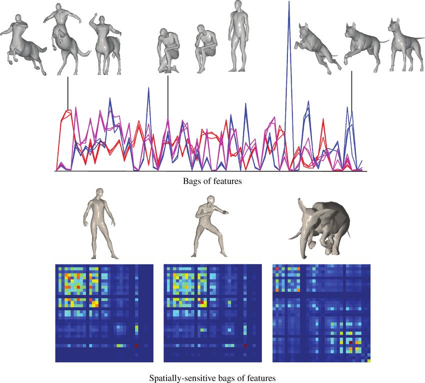
and retrieval of 3D shapes remains a challenging problem. Shape ity (Figure 1), and the aim of a successful retrieval approach is
retrieval based on text metadata (annotations and tags added by to be insensitive to such changes while maintaining high discrim-
humans) is often not capable of providing the same experience as a inative power. Significant advances have been made in designing
text search engine [Min et al. 2004]. efficient image retrieval techniques (see an overview in Veltkamp
Content-based shape retrieval using the shape itself as a query and and Hagedoorn [2001]), but the majority of 2D retrieval methods
based on the comparison of the geometric and topological properties do not immediately generalize to 3D shape retrieval [Tangelder and
of shapes is complicated by the fact that many 3D objects manifest Veltkamp 2008].
Authors’ addresses: A. M. Bronstein, Department of Electrical Engineering, Tel-Aviv University; M. M. Bronstein, Institute of Computational Science, Faculty
of Informatics, Università della Svizzera Italiana; L. J. Guibas, Department of Computer Science, Stanford University, Stanford, CA 94305; M. Ovsjanikov
(corresponding author), Institute for Computational and Mathematical Engineering, Stanford University, Stanford, CA 94305; email: maks@stanford.ecu.
Permission to make digital or hard copies of part or all of this work for personal or classroom use is granted without fee provided that copies are not made
or distributed for profit or commercial advantage and that copies show this notice on the first page or initial screen of a display along with the full citation.
Copyrights for components of this work owned by others than ACM must be honored. Abstracting with credit is permitted. To copy otherwise, to republish, to
post on servers, to redistribute to lists, or to use any component of this work in other works requires prior specific permission and/or a fee. Permissions may be
requested from Publications Dept., ACM, Inc., 2 Penn Plaza, Suite 701, New York, NY 10121-0701 USA, fax +1 (212) 869-0481, or permissions@acm.org.
c 2011 ACM 0730-0301/2011/01-ART1 $10.00 DOI 10.1145/1899404.1899405 http://doi.acm.org/10.1145/1899404.1899405
ACM Transactions on Graphics, Vol. 30, No. 1, Article 1, Publication date: January 2011.
1:2       •       A. M. Bronstein et al.

                                                                                           In Strecha et al. [2010], similarity-sensitive hashing algorithms were
                                                                                           applied to local SIFT descriptors to improve the performance of
                                                                                           feature matching in wide-baseline stereo reconstruction problems.
                                                                                              Behmo et al. [2008] showed that one of the disadvantages of the
                                                                                           bag of features approaches is that they lose information about the
                                                                                           spatial location of features in the image, and proposed the commute
                                                                                           graph representation, which partially preserves the spatial infor-
                                                                                           mation. An extension of this work based on the construction of
                                                                                           vocabularies of spatial relations between features was proposed in
                                                                                           Bronstein and Bronstein [2010a].
                                                                                              The success of feature-based methods in the computer vision
                                                                                           community is the main inspiration for the current article, where we
                                                                                           present a similar paradigm for 3D shapes.

Fig. 1. Examples of invariant image (top) and shape (bottom) retrieval.                    1.1   Related Works in the Shape Analysis Community
Shown on the left is a query, and on the right a few examples of desired
correct matches retrieved from a large database. Transformations shown in                  Shape retrieval is an established research area with many approaches
image retrieval are viewpoint variation, different illumination, background                and methods. For a detailed recent review, we refer the reader to
variation, occlusion, and partially missing data; in shape retrieval, different            Tangelder and Veltkamp [2008]. In rigid shape retrieval, global
nonrigid shape deformations are shown.                                                     descriptors based on volume and area [Zhang and Chen 2001],
                                                                                           wavelets [Paquet et al. 2000], statistical moments [Kazhdan et al.
                                                                                           2003; Novotni and Klein 2003; Tal et al. 2001], self-similarity (sym-
   Recently, feature-based methods have gained popularity in the                           metry) [Kazhdan et al. 2004], and distance distributions [Osada et al.
computer vision and pattern recognition communities with the in-                           2002] were used. Methods reducing the 3D shape retrieval to image
troduction of the Scale-Invariant Feature Transform (SIFT) [Lowe                           retrieval use 2D views [Funkhouser et al. 2003; Chen et al. 2003],
2004] and similar algorithms [Matas et al. 2004; Bay et al. 2006].                         slices [Jiantao et al. 2004], and silhouette and contour descriptors
The ability of these methods to demonstrate sufficiently good per-                         [Napoléon et al. 2007]. Graph-based methods based on skeletons
formance in many settings, including object recognition and image                          [Sundar et al. 2003] and Reeb graphs [Hilaga et al. 2001; Biasotti
retrieval, and the public availability of the code made SIFT-like ap-                      et al. 2003; Tung and Schmitt 2005] are capable of dealing with de-
proaches a commodity and a de facto standard in a variety of image                         formations, for example, matching articulated shapes. Lipman and
analysis tasks.                                                                            Funkhouser [2009] proposed the Möbius voting scheme for sparse
   One of the strengths of feature-based approaches in image re-                           shape matching.
trieval is that they allow one to think of an image as a collection                           Isometric shape deformations were first explicitly addressed by
of primitive elements (visual “words”), and use the well-developed                         Elad and Kimmel [2001, 2003]. The authors used MultiDimen-
methods from text search such as the “bag of features” paradigm.                           sional Scaling (MDS) [Borg and Groenen 1997; Bronstein et al.
One of the best implementations of these ideas is Video Google, a                          2006] to construct a representation of the intrinsic geometry of
Web application for object search in large collections of images and                       shapes (captured as a matrix of interpoint geodesic distances and
videos developed at Oxford University by Zisserman and collab-                             referred to as canonical forms) in a low-dimensional Euclidean
orators [Sivic and Zisserman 2003; Chum et al. 2007], borrowing                            space. A moment-based shape descriptor [Tal et al. 2001] was
its name through an analogy with the famous text search engine.                            then applied to obtain a shape signature. The method of Elad and
Video Google makes use of feature detectors and descriptors to rep-                        Kimmel was extended in Mémoli and Sapiro [2005] and Bron-
resent an image as a collection of visual words indexed in a “visual                       stein et al. [2006b, 2006a] to compare shapes as metric spaces us-
vocabulary.” Each image is compactly encoded into a vector of fre-                         ing the Gromov-Hausdorff distance [Gromov 1981], which tries to
quencies of occurrences of visual words, a representation referred to                      find the minimum-distortion correspondence between two shapes.
as a “bag of features.” Images containing similar visual information                       Numerically, the Gromov-Hausdorff distance computation can be
tend to have similar bags of features, and thus comparing bags of                          carried out using a method similar to MDS [Bronstein et al.
features allows retrieving similar images.                                                 2006b] or graph labeling [Torresani et al. 2008; Wang et al.
   Zisserman et al. showed that employing weighting schemes for                            2010]. In follow-up works, extensions of the Gromov-Hausdorff
bags of features that take into consideration the average occurrence                       distance used diffusion geometries [Bronstein et al. 2010d], dif-
of visual words in the whole database allows for very accurate re-                         ferent distortion criteria [Mémoli 2007, 2009], local photometric
trieval [Sivic and Zisserman 2003; Chum et al. 2007]. Since the com-                       [Thorstensen and Keriven 2009] and geometric [Dubrovina and
parison of bags of features usually boils down to finding weighted                         Kimmel 2010; Wang et al. 2010] data, and third-order [Zeng
correlation between vectors, such a method is suitable for indexing                        et al. 2010] distortion terms. While allowing for very accurate
and searching very large (Internet-scale) databases of images.                             and theoretically isometry-invariant shape comparison, the main
   In a follow-up work, Grauman et al. [Jain et al. 2008] showed                           drawback of the Gromov-Hausdorff framework is that it is based
that an optimal weighting of bags of features can be learned from                          on computationally expensive optimization. As a result, such meth-
examples of similar and dissimilar images using metric learning                            ods are mostly suitable for one-to-one or one-to-few shape retrieval
approaches [Torralba et al. 2008]. Shakhnarovich [2005] proposed                           cases, even though there have been recent attempts to overcome this
the similarity-sensitive hashing, which regards metric learning as a                       difficulty using Gromov-Hausdorff stable invariants [Chazal et al.
boosted classification problem. This method appeared very efficient                        2009a], which can be computed efficiently in practice.
in learning invariance to transformations in the context of video                             Reuter et al. [2005, 2009] proposed using Laplace-Beltrami
retrieval [Bronstein et al. 2010c]. In Bronstein et al. [2010e], an                        spectra (eigenvalues) as isometry-invariant shape descriptors. The
extension of this approach to the multimodal setting was presented.                        authors noted that such descriptors are invariant to isospectral
ACM Transactions on Graphics, Vol. 30, No. 1, Article 1, Publication date: January 2011.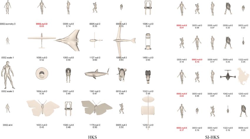
Shape Google: Geometric Words and Expressions for Invariant Shape Retrieval                                   •      1:3

                                                    Fig. 2. Flow of the ShapeGoogle algorithm.

shape transformations, a family theoretically larger than isometries.       statistical weighting scheme similar to Sivic and Zisserman [2003]
Rustamov [2007] used an isometry-invariant shape embedding sim-             and Chum et al. [2007] was also used to define point-wise signifi-
ilar to the eigenmaps proposed in Bérard et al. [1994], Belkin and         cance measure in the problem of partial shape matching. Ben-Chen
Niyogi [2003], and Lafon [2004] to create shape representations in          et al. [2008] use conformal factors as isometry-invariant local de-
the Euclidean space similar in spirit to canonical forms. He used           scriptors. Zaharescu et al. [2009] proposed a SIFT-like descriptor
histograms of Euclidean distances (using the approach of Osada              applied to functions defined on manifolds. Sun et al. [2009] in-
et al. [2002]) in the embedding space to compare the shapes. Shape          troduced deformation-invariant descriptors based on diffusion heat
similarity based on the comparison of histograms of diffusion dis-          kernels (referred to as Heat Kernel Signatures or HKS). More re-
tances were used as by Mahmoudi and Sapiro [2009]. In Bronstein             cently, a Scale-Invariant modification of these descriptors (SI-HKS)
et al. [2010d] and Bronstein and Bronstein [2009, 2010b], an inti-          were constructed in Bronstein and Kokkinos [2010] using local scale
mate relation between this method and the methods of Rustamov               normalization, and a volumetric Heat Kernel Signature (vHKS) was
[2007] was shown, and Bronstein and Bronstein [2010b] showed                proposed in Raviv et al. [2010b]. These former two approaches
a more general framework of which Mahmoudi and Sapiro [2009]                (HKS and SI-HKS) are adopted here for their discriminativity and
and Rustamov [2007] are particular cases.                                   efficient computability.
   Mémoli [2009] formulated a proper metric between shapes based
on a spectral variant of the Gromov-Wasserstein distance, and               1.2 Main Contribution
showed that shape similarity measures of Reuter et al. [2005],
Rustamov [2007], and Sun et al. [2009] can be viewed as a hi-               In this article, we bring the spirit of feature-based computer vision
erarchy of lower bounds of this metric.                                     approaches to the problem of nonrigid shape search and retrieval.
   Local feature-based methods are less common in the shape                 By analogy to Zisserman’s group works, we call our method Shape
analysis community than in computer vision, as there is nothing             Google. The present article is an extended version of Ovsjanikov
equivalent to a robust feature descriptor like SIFT to be univer-           et al. [2009], where the approach was first introduced. While work-
sally adopted. We see a few possible reasons. First, one of the             ing on this article, we discovered that the use of bags of features for
important properties of SIFT is its discriminativity combined with          shape representation has been independently developed by Toldo
robustness to different image transformations. Compared to                  et al. [2009].
images, shapes are usually known to be poorer in features, and thus            In this article, we first show a feature detector and descriptor
descriptors are less informative. Secondly, unlike images where             based on heat kernels of the Laplace-Beltrami operator, inspired by
invariance is usually limited to affine transformations, the degree of      Sun et al. [2009]. Descriptors are used to construct a vocabulary of
invariance required for shapes is usually much larger and includes          geometric words, distributions over which serve as a representation
nonrigid and topology-changing deformations.                                of a shape. This representation is invariant to isometric deforma-
   Feature-based methods have been explored by Pauly et al. [2003]          tions, robust under a wide class of perturbations, and allows one
for nonphotorealistic rendering. The authors detect multiscale ro-          to compare shapes undergoing different deformations. Second, we
bust contour features (somewhat analogous to edges in images).              show that taking into consideration the spatial relations between
A similar approach was proposed in Kolomenkin et al. [2009]. In             features in an approach similar to commute graphs [Behmo et al.
Mitra et al. [2010], local features were used to detect shape self-         2008] allows improving the retrieval performance. Finally, adopt-
similarity and grid-like structures. Local moments [Clarenz et al.          ing metric learning techniques widely used in the computer vision
2004] and volume descriptors [Gelfand et al. 2005] have been also           community [Jain et al. 2008], we show how to represent shapes as
proposed for rigid shape retrieval and correspondence. Shilane and          compact binary codes that can be efficiently indexed and compared
Funkhauser [2006] use a learnable feature detector and descriptor           using the Hamming distance.
maximizing the likelihood of correct retrieval, based on spherical             Figure 2 depicts a flow diagram of the presented approach. The
harmonics and surface area relative to the center of mass. Mitra            shape is represented as a collection of local feature descriptors
et al. [2006] proposed a patch-based shape descriptor and showed            (either dense or computed at a set of stable points following an
its application to shape retrieval and comparison. They also showed         optional stage of feature detection). The descriptors are then repre-
an efficient hashing scheme of such descriptors. An approach sim-           sented by “geometric words” from a “geometric vocabulary” using
ilar to the one presented in this article was presented in Li et al.        vector quantization, which produces a shape representation as a
[2006] for rigid shapes.                                                    bag of geometric words or pairs of words (expressions). Finally,
   Relatively few feature-based methods are invariant to isomet-            similarity-sensitive hashing is applied to the bags of features. We
ric deformations by construction. Raviv et al. [2007] and Bronstein         emphasize that the presented approach is generic, and different
et al. [2009] used histograms of local geodesic distances to construct      descriptor and detectors can be used depending on the application
an isometry-invariant local descriptor. In Bronstein et al. [2009],         demands.
                                                                         ACM Transactions on Graphics, Vol. 30, No. 1, Article 1, Publication date: January 2011.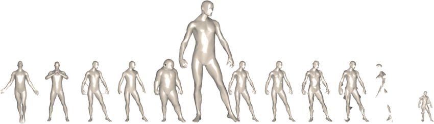
1:4       •       A. M. Bronstein et al.

   The rest of this article is organized as follows. In Section 2, we
start with a brief overview of feature-based approaches in com-
puter vision, focusing on methods employed in Video Google. In
Section 3, we formulate a similar approach for shapes. We show
how to detect and describe local geometric features. In Section 4, we
describe the construction of bags of geometric words. In Section 5,
we explore metric learning techniques for representing shapes as
short binary codes using Hamming embedding. Section 6 shows
experimental results, and Section 7 concludes.

2.    BACKGROUND: FEATURE-BASED METHODS
      IN COMPUTER VISION
The construction of a feature-based representation of an image typ-
ically consists of two stages, feature detection and feature descrip-
tion, often combined into a single algorithm. The main goal of a                           Fig. 3. Representation of text (left) and images (right) using the bags of
feature detector is to find stable points or regions in an image that                      features paradigm.
carry significant information on the one hand and can be repeatedly
found in transformed versions of the image on the other. Since there                       weight. The weight is expressed as the ratio of the term frequency
is no clear definition of what is a feature, different approaches can                      and the document frequency (referred to as term-frequency inverse
be employed. For example, in the SIFT method, feature points are                           document frequency or tf-idf in search engine literature). It was
located by looking for local maxima of the discrete image Lapla-                           shown in Sivic and Zisserman [2003] and Chum et al. [2007] that
cian (approximated as a difference of Gaussians) at different scales.                      this type of weighted distance is superior to simple, nonweighted,
SIFT uses linear scale-space in order to search for feature points that                    approach. In Jain et al. [2008], it was shown that an optimal weighted
appear at multiple resolutions of the image, which also makes the                          distance between bags of features on a given database can be learned
method scale-invariant [Lowe 2004]. Maximum Stable Extremal                                by supervised learning from examples of similar and dissimilar
Region (MSER) algorithm finds level sets in the image which ex-                            images.
hibit the smallest variation of area when traversing the level-set                            A few recent papers tried to extend bags of features by taking
graph [Matas et al. 2004; Kimmel et al. 2010]. Finally, it is possi-                       into consideration spatial information about the features. Marszalek
ble to select all the points in the image or a regular subsampling                         and Schmid [2006] used spatial weighting to reduce the influence
thereof as the set of features (in the latter case, the detector is usually                of background clutter (a similar approach was proposed in Leibe
referred to as dense [Tola et al. 2008]).                                                  et al. [2004]). Grauman and Darrell [2005] proposed comparing
   The next stage is feature description. A feature descriptor uses a                      distributions of local features using Earth Mover’s Distance (EMD)
representation of local image information in the neighborhood of                           [Rubner et al. 2000], which incorporates spatial distances. In
each feature point. For example, SIFT assigns a 128-dimensional                            Lazebnik et al. [2006], the spatial structure of features was captured
descriptor vector constructed as local histograms of image gradient                        using a multiscale bag of features construction. The representation
orientations around the point. The descriptor itself is oriented by                        proposed in Amores et al. [2007] used spatial relations between
the dominant gradient direction, which makes it rotation-invariant                         parts.
[Lowe 2004]. A similar approach, Speeded Up Robust Feature                                    Behmo et al. [2008] proposed a generalization of bags of fea-
(SURF) transform [Bay et al. 2006], uses a 64-dimensional de-                              tures that takes into consideration the spatial relations between the
scriptor, computed efficiently using integral images. At this stage,                       features in the image. In this approach, following the stage of fea-
the image can be compactly represented by specifying the spatial                           ture detection and description, a feature graph is constructed. The
coordinates of the detected feature points together with the cor-                          connectivity of the graph is determined by the spatial distance and
responding descriptors, which can be presented as vectors. This                            visual similarity of the features (spatially and visually close features
information allows, for example, finding correspondence between                            are connected). Next, the graph is collapsed by grouping together
images by matching their descriptors [Lowe 2004].                                          features whose descriptors are quantized to the same index in the
   In order to reduce the representation size, a vocabulary is con-                        visual vocabulary. The connections in the collapsed graph repre-
structed by performing vector quantization in the descriptor space.                        sent the commute time between the graph nodes. This graph can
Descriptors can be replaced by indices in the vocabulary repre-                            be considered an extension of a bag of features, where there is ad-
senting visual “words.” Typical vocabulary size can vary from a                            ditional information about the relations between the visual words.
few thousand [Sivic and Zisserman 2003] up to one million words                            In Bronstein and Bronstein [2010a], images were described as his-
[Chum et al. 2007]. Aggregating all the indices into a histogram                           tograms of pairs of features and the spatial relations between them
by counting the frequency of appearance of each visual word, the                           (referred to as visual expressions), using a visual vocabulary and a
bag of features (sometimes also called bag of visual terms or bag of                       vocabulary of spatial relations.
visterms) is constructed (Figure 3).
   After the feature detection and description stages, two images                          3.   LOCAL FEATURES IN SHAPES
can be compared by comparing their bags of features. This way, the
image similarity problem is reduced to the problem of comparing                            Trying to adapt feature-based approached to 3D shapes, one needs
vectors of feature frequencies. Typically, weighted correlation or                         to have the following in mind. First, the type of invariance in non-
weighted Euclidean distance is used to measure similarity of bags                          rigid shapes is different from one required in images. Typically,
of features. The weights can be chosen in such a way that features                         feature detectors and descriptors in images are made invariant to
frequent in the query shape (high term frequency) and infrequent in                        affine transformations, which accounts for different possible views
the entire database (low document frequency) are assigned a large                          of an object captured in the image. In case of nonrigid shapes, the
ACM Transactions on Graphics, Vol. 30, No. 1, Article 1, Publication date: January 2011.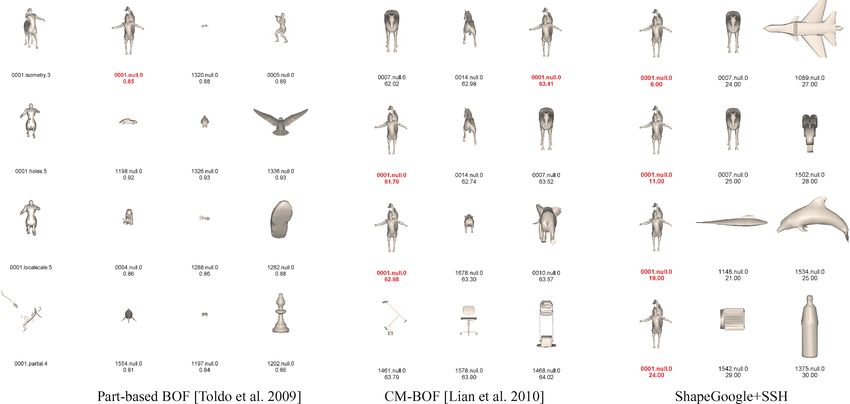
Shape Google: Geometric Words and Expressions for Invariant Shape Retrieval                                    •      1:5

richness of transformations is much larger, including changes in
pose, bending, and connectivity. Since many natural shape deforma-
tions such as articulated motion can be approximated by isometries,
basing the shape descriptors on intrinsic properties of the shape will
make it invariant to such deformations. Second, shapes are typi-
cally less rich in features than images, making it harder to detect
a large number of stable and repeatable feature points. This poses
a challenging trade-off in feature detection between the number of
features required to describe a shape on one hand and the number of
features that are repeatable on the other, and motivates our choice
to avoid feature detection at all and use dense descriptors instead.
Third, unlike images which in the vast majority of applications
appear as matrices of pixels, shapes may be often represented as              Fig. 4. Values of Kt (x, x) mapped on the shape (left) and values of Kt (x, y)
triangular meshes, point clouds, voxels, level sets, etc. Therefore,          for three different choices of y (marked with black dots in three rightmost
it is desirable to have local features computable across multiple             figures). The value t = 1024 is used. Hotter colors represent smaller values.
representations. Finally, since shapes usually do not have a global
system of coordinates, the construction of spatial relations between
features is a challenging problem.
                                                                              deformation-invariant, which makes it disadvantageous in nonrigid
   There exists a plethora of local shape detection and description
                                                                              shape analysis applications.
algorithms, and shortly we overview some of them. The reader is
                                                                                 Spin images. Perhaps one of the best known classes of feature
referred to the review paper [Bustos et al. 2005] and the recent
                                                                              descriptors are spin images [Johnson and Hebert 1999; Andreetto
benchmarks [Bronstein et al. 2010a, 2010b] for additional details.
                                                                              et al. 2004; Assfalg et al. 2007], which describe the neighborhood
                                                                              of a point by fitting a tangent plane to the surface at the point, and
3.1    Feature Detectors                                                      accumulating information about the neighborhood into 2D images
                                                                              which can then be directly compared. Although these methods can
Harris 3D. An effective feature detection method, called the Harris           be robust with respect to noise and changes in triangulation, they
operator, first proposed in images [Harris and Stephens 1988] was             were originally developed for rigid shape comparison, and are thus
extended to 3D shapes by Glomb [2009] and Sipiran and Bustos                  very sensitive to nonrigid shape deformations.
[2010]. This method is based on measuring variability of the shape               Mesh HOG. Zaharescu et al. [2009] use the histogram of gra-
in a local neighborhood of the point, by fitting a function to the            dients of a function defined in a local neighborhood of a point, as
neighborhood and identifying feature points as points where the               a point descriptor (similar to the Histogram Of Gradients (HOG)
derivatives of this function are high [Bronstein et al. 2010a].               [Dalal and Triggs 2005] technique used in computer vision). Though
   Mesh DOG. Several methods for feature detection have been in-              Zaharescu et al. show insensitivity of their descriptor to nonrigid
spired by the the difference of Gaussians (DOG), a classical feature          deformations, the fact that it is constructed based on k-ring neigh-
detection approach used in computer vision. Zaharescu et al. [2009]           borhoods makes it theoretically triangulation-dependent.
introduce the mesh DOG approach by first applying Gaussian fil-                  Heat Kernel Signatures (HKS). Recently, there has been in-
tering to functions (e.g., mean or Gauss curvature) defined on the            creased interest in the use of diffusion geometry for shape recogni-
shape. This creates a representation of the function in scale space,          tion [Rustamov 2007; Ovsjanikov et al. 2008; Mateus et al. 2008;
and feature points are prominent maxima of the scale space across             Mahmoudi and Sapiro 2009; Bronstein et al. 2010d; Raviv et al.
scales. Castellani et al. [2008] apply Gaussian filtering directly on         2010a]. This type of geometry arises from the heat equation
the mesh geometry, and use a robust method inspired by Itti et al.
[1998] to detect feature points as points with greatest displacement                                             ∂
in the normal direction.                                                                                 X +        u = 0,                       (1)
                                                                                                                ∂t
   Heat kernel feature detectors. Recently, Sun et al. [2009] and
Gebal et al. [2009] introduced feature detection methods based on             which governs the conduction of heat u on the surface X (here,
the heat kernel. These methods define a function on the shape,                X denotes the negative semidefinite Laplace-Beltrami operator,
measuring the amount of heat remaining at a point x after large               a generalization of the Laplacian to non-Euclidean domains). The
time t given a point source at x at time 0, and detect features as local      fundamental solution Kt (x, z) of the heat equation, also called the
maxima of this function. As these methods are intimately related to           heat kernel, is the solution of (1) with a point heat source at x (see
our work, we discuss in depth the properties of heat kernels in the           Figure 4). Probabilistically, the heat kernel can also be interpreted
following section.                                                            as the transition density function of a Brownian motion (continuous
                                                                              analog of a random walk) [Hsu 2002; Coifman and Lafon 2006;
                                                                              Lafon 2004].
3.2    Feature Descriptors                                                       Sun et al. [2009] proposed using the diagonal of the heat kernel
Shape context. Though originally proposed for 2D shapes and                   as a local descriptor, referred to as the Heat Kernel Signatures
images [Belongie et al. 2002], shape context has also been gener-             (HKS). For each point x on the shape, its heat kernel signature is
alized to 3D shapes. For a point x on a shape X, the shape context            an n-dimensional descriptor vector of the form
descriptor is computed as a log-polar histogram of the relative coor-                         p(x) = c(x)(Kt1 (x, x), . . . , Ktn (x, x)),                     (2)
dinates of the other points (x  − x) for all x  ∈ X. Such a descriptor
is translation-invariant and can be made rotation-invariant. It is            where c(x) is chosen in such a way that p(x)2 = 1.
computable on any kind of shape representation, including point                 The HKS descriptor has many advantages, which make it a fa-
clouds, voxels, and triangular meshes. It is also known to be in-             vorable choice for shape retrieval applications. First, the heat ker-
sensitive to small occlusions and distortion, but in general is not           nel is intrinsic (i.e., expressible solely in terms of the Riemannian
                                                                           ACM Transactions on Graphics, Vol. 30, No. 1, Article 1, Publication date: January 2011.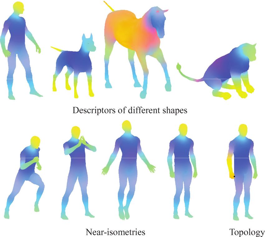
1:6       •       A. M. Bronstein et al.

                                                                                           of transformations
                                                                                                    pdif (x) = (log Kατ2 (x, x) − log Kατ1 (x, x), . . . ,
                                                                                                               log Kατ m (x, x) − log Kατm−1 (x, x)),
                                                                                                      p̂(x) = |(F pdif (x))(ω1 , . . . , ωn )|,                  (3)
                                                                                           where F is the discrete Fourier transform, and ω1 , . . . , ωn denotes
                                                                                           a set of frequencies at which the transformed vector is sampled.
                                                                                           Taking differences of logarithms removes the scaling constant, and
                                                                                           the Fourier transform converts the scale-space shift into a complex
                                                                                           phase, which is removed by taking the absolute value. Typically,
                                                                                           a large m is used to make the representation insensitive to large
                                                                                           scaling factors and edge effects. Such a descriptor was dubbed
                                                                                           Scale-Invariant HKS (SI-HKS) [Bronstein and Kokkinos 2010].

                                                                                           3.3    Numerical Computation of HKS
                                                                                           For compact manifolds, the Laplace-Beltrami operator has a discrete
                                                                                           eigendecomposition of the form
                                                                                                                       −X φl = λl φl ,                          (4)
                                                                                           where λ0 = 0 ≥ λ1 ≥ λ2 . . . are eigenvalues and φ0 = const, φ1 , . . .
Fig. 5. An RGB visualization of the first three components of the HKS de-                  are the corresponding eigenfunctions. The heat kernel can be written
scriptor of different shapes (top row) and transformations of the same shape               in the following form Jones et al. [2008]
(bottom row). Four leftmost shapes in the bottom row are approximately
isometric, and the descriptor appears to be invariant to these deformations.
                                                                                                                              ∞

The rightmost shape in the bottom row has different topology (hand and leg                                   Kt (x, x  ) =         e−λl t φl (x)φl (x  ).      (5)
are glued at point marked with black dot). Note that though the descriptor                                                    l=0

changes in the area of the topological change, the discrepancy is localized.               Since the coefficients decay exponentially as λi increase, for large
                                                                                           values of t we can approximate the HKS as
structure of X), and thus invariant under isometric deformations
                                                                                                                               k
of X. This makes HKS deformation-invariant (Figure 5, bottom                                                    Kt (x, x) ≈           e−λl t φl (x)2 .           (6)
row left). Second, such a descriptor captures information about the                                                             l=0
neighborhood of a point x on the shape at a scale defined by t. It
captures differential information in a small neighborhood of x for                         Thus, in practice, the computation of the HKS descriptor boils down
small t, and global information about the shape for large values                           to computing the first largest eigenvectors and eigenvalues of the
of t. Thus, the n-dimensional feature descriptor vector p(x) can                           Laplace-Beltrami operator. For small values of t, this computation
be seen as analogous to the multiscale feature descriptors used in                         of HKS is numerically unstable, an issue that has been recently
the computer vision community. Third, for small scales t, the HKS                          addressed in Vaxman et al. [2010] using a multiresolution approach.
descriptor takes into account local information, which makes topo-                            Discrete eigendecomposition problem. In the discrete setting,
logical noise have only local effect (Figure 5, bottom row right).                         having the shape represented by a finite sampling X̂ = {x1 , . . . , xN },
Fourth, Sun et al. prove that if the Laplace-Beltrami operator of                          several variants of the Laplace-Beltrami operator can be expressed
a shape is nondegenerate (does not contain repeated eigenvalues),                          in the following generic form
then any continuous map that preserves the HKS at every point must                                                         1
be an isometry. This latter property led Sun et al. to call the HKS                                            (X̂ f )i =      wij (fi − fj ),                  (7)
                                                                                                                           ai j
provably informative. Finally, as will be shown next, the compu-
tation of the HKS descriptor relies on the computation of the first
                                                                                           where f : X̂ = f (xi ) is a scalar function defined on X̂, wij are
eigenfunctions and eigenvalues of the Laplace-Beltrami operator,
                                                                                           weights, and ai are normalization coefficients. In matrix notation,
which can be done efficiently and across different shape represen-
                                                                                           Eq. (7) can be written as
tations. This makes HKS applicable to different geometric data,
though we focus in this article on shapes represented as triangular                                                  X̂ f = A−1 Wf,                           (8)
meshes.
    Scale-Invariant Heat Kernel Signatures (SI-HKS). A disadvan-                           where A = diag(ai ) and W = diag       l=i wil − (wij ), allowing one
tage of the HKS is its dependence on the global scale of the shape. If                     to find the discrete eigenfunctions and eigenvalues by solving the
X is globally scaled by β, the corresponding HKS is β −2 Kβ −2 t (x, x).                   generalized eigendecomposition [Lévy 2006]
It is possible in theory to perform global normalization of the shape                                                  W       =A            ,                   (9)
(e.g., normalizing the area or Laplace-Beltrami eigenvalues), but
such a normalization is impossible if the shape has, for example,                          where is the (k + 1) × (k + 1) diagonal matrix of eigenvalues and
missing parts. As an alternative, a local normalization was pro-                              is an N × (k + 1) matrix of the corresponding eigenvectors, such
posed in Bronstein and Kokkinos [2010] based on the properties of                          that il ≈ φl (xi ).
the Fourier transform. By using a logarithmic scale-space t = α τ ,                           Laplace-Beltrami operator discretization. Different discretiza-
global scaling results in HKS amplitude scaling and shift by 2 logα β                      tions of the Laplace-Beltrami lead to different choice of A and W
in the scale-space. This effect is undone by the following sequence                        [Zhang 2004; Floater and Hormann 2005; Bobenko and Springborn
ACM Transactions on Graphics, Vol. 30, No. 1, Article 1, Publication date: January 2011.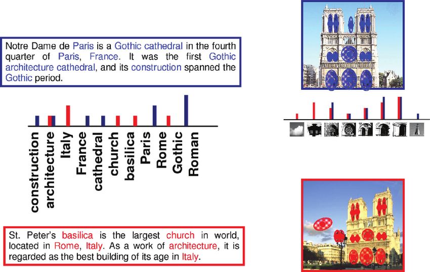
Shape Google: Geometric Words and Expressions for Invariant Shape Retrieval                                         •      1:7

2007]. For triangular meshes, a popular choice adopted in this arti-                       a V × 1 vector whose elements are
cle is the cotangent weight scheme [Pinkall and Polthier 1993] and                                                                           p(x)−pi 2
its variants [Meyer et al. 2003], in which wij = (cot αij + cot βij )/2                                               θi (x) = c(x)e
                                                                                                                                         −
                                                                                                                                                 2σ 2
                                                                                                                                                       2
                                                                                                                                                           ,              (12)
for j in the 1-ring neighborhood of vertex i and zero otherwise,
where αij and βij are the two angles opposite to the edge between                          and the constant c(x) is selected in such a way that θ (x)1 = 1.
vertices i and j in the two triangles sharing the edge. It can be                          θi (x) can be interpreted as the probability of the point x to be
shown [Wardetzky et al. 2008] that this discretization preserves                           associated with the descriptor pi from the vocabulary P.
many important properties of the continuous Laplace-Beltrami op-                               Eq. (12) is a “soft” version of vector quantization. “Hard” vector
erator, such as positive semidefiniteness, symmetry, and locality.                         quantization is obtained as a particular case of (12) by choosing
For shapes represented as point clouds, the discretization of Belkin                       σ ≈ 0, in which case θi (x) = 1 (where i is the index of the
et al. [2009] can be used.                                                                 vocabulary element pi closest to p in the descriptor space) and zero
   Finite elements. Direct computation of the eigenfunction without                        otherwise.
explicit discretization of the Laplace-Beltrami operator is possible                           Integrating the feature distribution over the entire shape X yields
using the Finite Elements Method (FEM). By the Green formula, the                          a V × 1 vector
Laplace-Beltrami eigenvalue problem X φ = λφ can be expressed
in the weak form as                                                                                                   f(X) =            θ(x)dμ(x),                        (13)
                                                                                                                                    X
                       X φ, α     = λ φ, α L2 (X)
                                  L2 (X)                             (10)                  which we refer to as a Bag of Features (or BoF for short). Using
                                                                                          this representation, we can define a distance between two shapes X
for any smooth α, where f, g L2 (X) = X f (x)g(x)dμ(x) and μ(x)
is the standard area measure on X. Given a finite basis {α1 , . . . , αq }                 and Y as a distance between bags of features in IR V ,
spanning a subspace of L2 (X), the solution φ can be expanded                                                     dBoF (X, Y ) = f(X) − f(Y ).                          (14)
as φ(x) ≈ u1 α1 (x) + · · · + uq αq (x). Substituting this expansion
into (10) results in a system of equations                                                 An example of bags of features using a vocabulary of size 64 is
                                                                                           shown in Figure 7 (top).

           q

                                                q
                  uj X αj , αr   L2 (X)   =λ          uj α j , α r   L2 (X) ,
                                                                                           4.1 Spatially Sensitive Bags of Features
           j =1                                 j =1
                                                                                           The disadvantage of bags of features is the fact that they consider
for r = 1, . . . , q, which, in turn, is posed as a generalized eigenvalue                 only the distribution of the words and lose the relations between
problem                                                                                    them. Resorting again to a text search example, in a document
                                  Au = λBu.                                      (11)      about “matrix decomposition” the words “matrix” and “decompo-
                                                                                           sition” are frequent. Yet, a document about the movie Matrix and a
(here A and B are q × q matrices with elements arj =                                       document about decomposition of organic matter will also contain
 X αj , αr L2 (X) and brj = αj , αr L2 (X) ). Solution of (11) gives                      these words, which will result in a similar word statistics and, con-
eigenvalues λ and eigenfunctions φ = u1 α1 + · · · + uq αq of X .                         sequently, similar bags of features. In the most pathological case, a
   As the basis, linear, quadratic, or cubic polynomials defined on                        random permutation of words in a text will produce identical bags
the mesh can be used. The FEM approach is quite general, and in                            of words. In order to overcome this problem, text search engines
particular, the cotangent scheme can be derived as its instance by                         commonly use vocabularies consisting not only of single words but
using piecewise linear hat functions centered on the vertices and                          also of combinations of words or expressions. The combination of
supported within the 1-ring neighborhood. Since the inner products                         words “matrix decomposition” will be thus frequently found in a
in FEM are computed on the surface, the method can be less sensitive                       document about the algebraic notion, but unlikely in a document
to the shape discretization than the direct approach based on the                          about the Matrix movie (Figure 6).1
discretization of the Laplace-Beltrami operator. This is confirmed                            In case of shapes, the phenomenon may be even more pro-
by numerical studies performed by Reuter et al. who showed the                             nounced, as shapes, being poorer in features, tend to have many
advantage in accuracy of higher-order FEM schemes at the expense                           similar geometric words. The analogy of expressions in shapes
of computational and storage complexity [Reuter et al. 2005]. In                           would be sets of spatially close geometric words. Instead of look-
Bronstein et al. [2010b], linear FEM method produced comparable                            ing at the frequency of individual geometric words, we look at the
results in the discretization of HKS compared to cotangent weights                         frequency of word pairs, thus accounting not only for the frequency
(note that the sole difference between these methods is the use of a                       but also for the spatial relations between features. For this purpose,
lumped mass matrix to get a diagonal matrix A for the latter).                             we define the following generalization of a bag of features, referred
                                                                                           to as a Spatially Sensitive Bags of Features (SS-BoF).
4.   BAGS OF FEATURES
                                                                                                        F(X) =              θ(x)θ T (y)Kt (x, y)dμ(x)dμ(y)                (15)
Given local descriptor computed at a set of stable feature points                                                     X×X
(or alternatively, a dense descriptor), similarly to feature-based ap-
                                                                                           The resulting representation F is a V × V matrix, representing the
proaches in computer vision, our next step is to quantize the descrip-
                                                                                           frequency of appearance of nearby geometric words or “geometric
tor space in order to obtain a compact representation in a vocabulary
                                                                                           expressions” i, j . It can be considered as a bag of features in a
of “geometric words.” A vocabulary P = {p1 , . . . , pV } of size V
                                                                                           vocabulary of size V 2 consisting of pairs of words (see Figure 7,
is a set of representative vectors in the descriptor space, obtained
by means of unsupervised learning (vector quantization through
k-means).                                                                                  1 For this reason, Web search engines return different results when the search

   Given a vocabulary P, for each point x ∈ X with the descriptor                          string is written with quotation marks (“matrix decomposition”) and without
p(x), we define the feature distribution θ (x) = (θ1 (x), . . . , θV (x))T ,               (matrix decomposition).
                                                                                        ACM Transactions on Graphics, Vol. 30, No. 1, Article 1, Publication date: January 2011.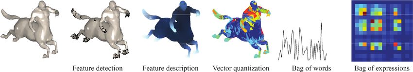
1:8       •       A. M. Bronstein et al.

                                                                                           common the term i is in the database, and so it is less likely to
                                                                                           be able to discriminate between shapes [Chum et al. 2007]. This
                                                                                           information can be taken into consideration when comparing bags
                                                                                           of features, by down-weighting common words. This leads to a
                                                                                           weighted L1 distance

                                                                                                                             V
                                                                                                          dBoFw (X, Y ) =            wi |fi (X) − fi (Y )|,       (18)
                                                                                                                             i=1

                                                                                           referred to as tf-idf weighting.
                                                                                              Statistical weighting can be applied in the same way to SS-BoFs.
                                                                                           In the computation of inverse document frequency, instead of geo-
Fig. 6. Example visualizing the importance of expressions. Shown left to
                                                                                           metric words, geometric expressions (pairs of words) are used. This
right: text about matrix decomposition in math; same text with randomly
                                                                                           way, common expressions are down-weighted.
shuffled words; text on biological process of decomposition; text about the
movie Matrix. All the texts have similar or even identical distributions of
words, shown as the left histogram. Yet, adding a vocabulary with combi-                   5.   SHAPES AS BINARY CODES
nations of words (expressions) allows one to distinguish between the texts                 Assume that we are given a class of transformations T (such as
(right histogram).                                                                         bending), invariance to which is desired in the shape retrieval prob-
                                                                                           lem. Theoretically, it is possible to construct the local descriptors
                                                                                           to be invariant under T , making the resulting bag of features rep-
bottom). When hard quantization is used (the vectors θ are binary),                        resentation, up to quantization errors, invariant as well. However,
the element Fij would be large if the instances of the words i and                         only simple geometric transformation can be modeled explicitly,
j are spatially close to each other on X (the diffusion distances                          and thus the descriptor would rarely be truly invariant to real shape
between words i and j is small, or alternatively, the heat kernel K                        transformations.
is large). fij can also be interpreted as the proximity of the words                          Metric learning. As an alternative, we propose learning the
i, j in the descriptor space and on the surface X, which is similar                        invariance from examples. Assume that we are given a set of bags
to the spirit of Behmo et al. [2008], and Bronstein and Bronstein                          of features (or spatially sensitive bags of features) F describing
[2010a].                                                                                   different shapes. We denote by P = {(f, f ◦ τ ) : f ∈ F , τ ∈ T } the
   We define a distance between two shapes X and Y as a distance                           set of positive pairs (bags of features of identical shapes, differing
between F(X) and F(Y ),                                                                    up to some transformation), and by N = {(f, f  ) : f = f  ∈ F } the
                                                                                           set of negative pairs (bags of features of different shapes). Negative
                    dSS−BoF (X, Y ) = F(X) − F(Y ).                         (16)         pairs are modeled by taking different shapes which are known to
                                                                                           be distinct. For positive pairs, it is usually possible to simulate
4.2     Statistical Weighting                                                              representative transformations from class T . Our goal is to find a
An important question is how to compare the bag of features rep-                           metric between bags of features that is as small as possible on the
resentations of two shapes. While deferring the question of con-                           set of positives and as large as possible on the set of negatives.
structing an optimal metric to the next section, we note that not all                         Similarity Sensitive Hashing (SSH). Shakhnarovich [2005] con-
geometric words are equally important for the purpose of shape re-                         sidered metrics parameterized as
trieval. In text retrieval, it is common to assign different weights to
                                                                                                     dA,b (x, x  ) = dH (sign(Af + b), sign(Af  + b)),           (19)
words according to their statistical importance. Frequent words in a

document are likely to be informative; on the other hand, in order to                      where dH (y, y ) = 2s − 12 si=1 sign(yi yi ) is the Hamming metric
be discriminative, they should be rare in the corpus of documents to                       in the s-dimensional Hamming space Hs = {−1, +1}s of binary
which the document belongs. Down-weighting common words like                               sequences of length s. A and b are an s × V matrix and an s × 1
prepositions and articles increases the performance of text search                         vector, respectively, parameterizing the metric. Our goal is to find
engines. Similar approaches have been successfully used for object                         A and b such that dA,b reflects the desired similarity of pairs of bags
retrieval in video [Sivic and Zisserman 2003], as well as 3D shape                         of features f, f  in the training set.
comparison [Shilane and Funkhauser 2006; Bronstein et al. 2009].                              Ideally, we would like to achieve dA,b (f, f  ) ≤ d0 for (f, f  ) ∈ P,
   Here, we use statistical weighting of bags of geometric features.                       and dA,b (f, f  ) > d0 for (f, f  ) ∈ N , where d0 is some threshold. In
In the case when hard quantization is used, a bag of features rep-                         practice, this is rarely achievable as the distributions of dA,b on P
resents the occurrence frequency of different geometric words in                           and N have cross-talks responsible for false positives (dA,b ≤ d0 on
the shape, referred to as term frequency. Assume we have a shape                           N ) and false negatives (dA,b > d0 on P). Thus, optimal A, b should
database of size D, containing the shapes X1 , . . . , XD . The inverse                    minimize
document frequency of geometric word i is defined as the logarithm
of the inverse fraction of the shapes in the database in which this                                                    1  sign(dA,b (f,f  )−d0 )
                                                                                                                 min               {e               }
word appears,                                                                                                     A,b |P|

                                                                                                                         (f,f )∈P

                                              D                                                                      1  sign(d0 −dA,b (f,f  ))
                   wi = log D                                 ,              (17)                                +        {e                    }.               (20)
                                                                                                                    |N |
                                      j =1 δ(fi (Xj ) > 0)                                                                (f,f )∈N

where δ is an indicator function, and fi (Xj ) counts the number                             In Shakhnarovich [2005], the learning of optimal parameters A, b
of occurrences of word i in shape j . The smaller is wi , the more                         was posed as a boosted binary classification problem, where dA,b
ACM Transactions on Graphics, Vol. 30, No. 1, Article 1, Publication date: January 2011.
Shape Google: Geometric Words and Expressions for Invariant Shape Retrieval                                      •      1:9

Fig. 7. Top row: examples of bags of features computed for different deformations of centaur (red), dog (blue), and human (magenta). Note the similarity of
bags of features of different transformations and dissimilarity of bags of features of different shapes. Also note the overlap between the centaur and human
bags of features due to partial similarity of these shapes. Bottom row: examples of spatially sensitive bags of features computed for different deformations of
human (left and center) and elephant (right).

acts as a strong binary classifier and each dimension of the lin-
ear projection sign(Ai x + bi ) is a weak classifier. This way, the                 Algorithm 1: Metric learning between bags of features using
AdaBoost algorithm can be used to progressively construct A and                     similarity sensitive hashing (SSH)
b, which is a greedy solution of (20). At the ith iteration, the ith                 Input: P pairs of bags of features (fp , fp ) labeled by
row of the matrix A and the ith element of the vector b are found                             sp = s(fp , fp ) ∈ {±1}.
minimizing a weighted version of (20). Weights of false positive                     Output: Parameters A, b of the optimal projection.
and false negative pairs are increased, and weights of true positive
and true negative pairs are decreased, using the standard AdaBoost                 1 Initialize weights wp1 = 1/P .
reweighting scheme [Freund and Schapire 1995], as summarized in                    2 for i = 1, . . . , d do
Algorithm 1.                                                                       3      Set the ith row of A and b by solving the
   Projection selection. Finding an optimal projection Ai at step 3                        optimization problem
of Algorithm 1 is difficult because of the sign function nonlinearity.                                          P
In Shakhnarovich [2005], a random projection was used at each                                  (Ai , bi ) = min  p=1 wp sp (2 − sign(Ai fp + bi ))
                                                                                                                      i
                                                                                                              Ai ,bi
step. In Bronstein et al. [2010c], is was shown empirically that a
better way is to select a projection by using the minimizer of the                                                            (2 − sign(Ai fp + bi )).
exponential loss of a simpler problem,                                                     Update weights

                                                                                           wpi+1 = wpi e−sp sign(Ai fp +bi )sign(Ai fp +bi ) and normalize by
                                         AT CN A                                           sum.
                       Ai = argmax               ,                    (21)
                                A=1    AT CP A
                                                                                                                                            −1     1
where CP and CN are the covariance matrices of the positive and                    (21) is the largest generalized eigenvector of CP 2 CN2 , which can be
negative pairs, respectively. It can be shown that Ai maximizing                   found by solving a generalized eigenvalue problem. This approach
                                                                               ACM Transactions on Graphics, Vol. 30, No. 1, Article 1, Publication date: January 2011.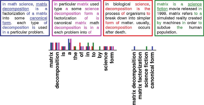
1:10        •      A. M. Bronstein et al.

is similar in its spirit to Linear Discriminative Analysis (LDA) and
was used in Bronstein et al. [2010c, 2010e]. Since the minimizers                               Algorithm 2: ShapeGoogle algorithm for shape retrieval
of (20) and (21) do not coincide exactly, in our implementation, we                              Input: Query shape X; geometric vocabulary
select a subspace spanned by the largest ten eigenvectors, out of                                        P = {p1 , . . . , pV }, database of shapes {X1 , . . . , XD }.
which the direction as well as the threshold parameter b minimizing                              Output: Shapes from {X1 , . . . , XD } most similar to X.
the exponential loss are selected. Such an approach appears more
                                                                                            1    if Feature detection then
efficient (in terms of bits required for the hashing to discriminate
                                                                                            2         Compute a set X  of stable feature points on X.
between dissimilar data) than Shakhnarovich [2005].
   Advantages. There are a few advantages to invariant metric learn-                        3    else
ing in our problem. First, unlike the tf-idf weighting scheme, which                        4         X = X.
constructs a metric between bags of features based on an empirical                          5 Compute local feature descriptor p(x) for all x ∈ X  .
evidence, the metric dA,b is constructed to achieve the best discrim-
                                                                                            6 Quantize the local feature descriptor p(x) in the vocabulary P,
inativity and invariance on the training set. The Hamming metric in
the embedding space can be therefore thought of as an optimal met-                            obtaining for each x a distribution θ(x) ∈ IR V .
ric on the training set. If the training set is sufficiently representative,                7 if Geometric expressions then
such a metric generalizes well. Secondly, the projection itself has an                      8     Compute a spatially-sensitive V × V bag of geometric
effect of dimensionality reduction, and results in a very compact rep-                            words
resentation of bags of features as bitcodes, which can be efficiently
stored and manipulated in standard databases. Third, modern CPU                                              F(X) =           θ(x)θ T (y)Kt (x, y)dμ(x)dμ(y),
                                                                                                                        X×X
architectures allow very efficient computation of Hamming dis-
tances using bit counting and SIMD instructions. Since each of the                                   and parse it into a V 2 × 1 vector f(X).
bits can be computed independently, shape similarity computation                            9 else
in a shape retrieval system can be further parallelized on multiple                        10      Compute a V × 1 bag of geometric words
CPUs using either shared or distributed memories. Due to the com-
pactness of the bitcode representation, search can be performed in
                                                                                                                           f(X) =         θ(x)dμ(x)
memory. Fourth, invariance to different kinds of transformations                                                                      X
can be learned. Finally, since our approach is a meta-algorithm, it                                  .
works with any local descriptor, and in particular, can be applied                         11 Embed the bag of words/expressions into the s-dimensional
to descriptors most successfully coping with particular types of                              Hamming space y(X) = sign(Af(X) + b) using pre-computed
transformations and invariance.                                                               parameters A, b.
   We summarize our shape retrieval approach in Algorithm 2.
                                                                                           12 Compare the bitcode y(X) to bitcodes y(X1 ), . . . , y(XD ) of the
                                                                                              shapes in the database using Hamming metric and find the
6.      RESULTS                                                                               closest shape.
6.1     Experimental Setup
Dataset. In order to assess our method, we used the SHREC 2010                              number corresponded to the transformation strength levels: the
robust large-scale shape retrieval benchmark, simulating a retrieval                        higher the number, the stronger the transformation (e.g., in noise
scenario in which the queries include multiple modifications and                            transformation, the noise variance was proportional to the strength
transformations of the same shape [Bronstein et al. 2010b]. The                             number). For scale transformations, the levels 1–5 corresponded
dataset used in this benchmark was aggregated from three public                             to scaling by the factor of 0.5, 0.875, 1.25, 1.625, and 2. For the
domain collections: TOSCA shapes [Bronstein et al. 2008], Robert                            isometry class, the numbers did not reflect transformation strength.
Sumner’s collection of shapes [Sumner and Popović 2004], and                               The total number of transformations per shape was 55, and the total
Princeton shape repository [Shilane et al. 2004]. The shapes were                           query set size was 715. Each query had one correct corresponding
represented as triangular meshes with the number of vertices ranging                        null shape in the dataset.
approximately between 300 and 30,000. The dataset consisted of                                 Evaluation criteria. Evaluation simulated matching of trans-
1184 shapes, out of which 715 shapes were obtained from 13 shape                            formed shapes to a database containing untransformed (null) shapes.
classes with simulated transformation (55 per shape) used as queries                        As the database, all 469 shapes with null transformations were used.
and 456 unrelated shapes, treated as negatives.2                                            Multiple query sets according to transformation class and strength
   Queries. The query set consisted of 13 shapes taken from the                             were used. For transformation x and strength n, the query set con-
dataset (null shapes), with simulated transformations applied to                            tained all the shapes with transformation x and strength ≤ n. In each
them. For each null shape, transformations were split into 11 classes                       transformation class, the query set size for strengths 1, 2, . . . , 5 was
shown in Figure 9: isometry (nonrigid almost inelastic deforma-                             13, 26, 39, 52, and 65. In addition, query sets with all transforma-
tions), topology (welding of shape vertices resulting in different                          tions broken down according to strength were used, containing 143,
triangulation), micro holes and big holes, global and local scaling,                        286, 429, 572, and 715 shapes (referred to as average in the follow-
additive Gaussian noise, shot noise, partial occlusion (resulting                           ing).
in multiple disconnected components), down sampling (less than                                 Performance was evaluated using precision/recall characteristic.
20% of original points), and mixed transformations. In each class,                          Precision P (r) is defined as the percentage of relevant shapes in
the transformation appeared in five different versions numbered                             the first r top-ranked retrieved shapes. In the present benchmark, a
1–5. In all shape categories except scale and isometry, the version                         single relevant shape existed in the database for each query. Mean
                                                                                            Average Precision (mAP), defined as
2 The
      datasets are available at http://tosca.cs.technion.ac.il/book/shrec                                         mAP =        P (r) · rel(r),
robustness.html.                                                                                                                 r

ACM Transactions on Graphics, Vol. 30, No. 1, Article 1, Publication date: January 2011.
You can also read