Production Optimisation 2018 - RVO.nl
←
→
Page content transcription
If your browser does not render page correctly, please read the page content below
Production Optimisation 2018

Per Valvatne, Leendert Geurtsen, Assaf Mar-Or, Gosia Kaleta, Jan Limbeck and Gerard Joosten
© EP2018 Dit rapport is een weerslag van een voortdurend studie- en dataverzamelingsprogramma en bevat de
stand der kennis van mei 2018. Het copyright van dit rapport ligt bij de Nederlandse Aardolie Maatschappij B.V.
Het copyright van de onderliggende studies berust bij de respectievelijke auteurs. Dit rapport of delen daaruit
mogen alleen met een nadrukkelijke status-en bronvermelding worden overgenomen of gepubliceerd.

                                                Page 2 of 98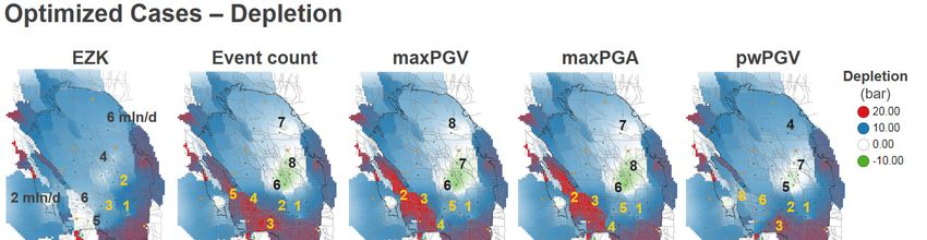
Table of Contents
1     Introduction .................................................................................................................................... 7
    1.1      Study background ................................................................................................................... 7
    1.2      Study objective........................................................................................................................ 8
    1.3      Report structure ...................................................................................................................... 9
2     Study setup ................................................................................................................................... 10
    2.1      Production induced seismicity cause and effect chain ......................................................... 10
    2.2      Model implementation ......................................................................................................... 10
    2.3      Model controls ...................................................................................................................... 11
    2.4      Objective functions ............................................................................................................... 13
      2.4.1          Practicability of a risk-based optimisation .................................................................... 13
      2.4.2          Event Count ................................................................................................................... 13
      2.4.3          Maximum Peak Ground Acceleration (maxPGA) and Peak Ground Velocity (maxPGV)
                     13
      2.4.4          Population weighted PGV (pwPGV) .............................................................................. 13
    2.5      Boundary conditions ............................................................................................................. 14
      2.5.1          Production profile ......................................................................................................... 14
      2.5.2          Production fractions...................................................................................................... 15
      2.5.3          Optimiser ...................................................................................................................... 15
    2.6      Subset of uncertainty tree .................................................................................................... 16
3     Hazard and Risk Model ................................................................................................................. 17
    3.1      Dynamic reservoir simulation model .................................................................................... 17
    3.2      Seismological model ............................................................................................................. 19
    3.3      Ground-Motion-Prediction Equation .................................................................................... 19
    3.4      Model uncertainty ................................................................................................................ 21
      3.4.1          Epistemic uncertainty ................................................................................................... 21
      3.4.2          Aleatoric uncertainty .................................................................................................... 22
    3.5      Model robustness ................................................................................................................. 22
      3.5.1          Robustness with respect to aleatoric uncertainty ........................................................ 22
      3.5.2          Robustness with respect to epistemic uncertainty....................................................... 24
4     Optimisation ................................................................................................................................. 27
    4.1      Setup ..................................................................................................................................... 27
      4.1.1          Controls ......................................................................................................................... 27
      4.1.2          Reference Case.............................................................................................................. 27

                                                                  Page 3 of 98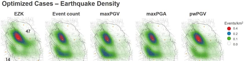
4.1.3         Optimisation window .................................................................................................... 27
    4.2      Results ................................................................................................................................... 27
5     Data driven analysis of model response ....................................................................................... 36
    5.1      Random Forest proxy models ............................................................................................... 36
    5.2      Sampling of the control space .............................................................................................. 36
    5.3      Overall model quality assessment ........................................................................................ 37
    5.4      Random Forest model analysis ............................................................................................. 39
    5.5      Observations from Random Forest models .......................................................................... 47
    5.6      Consistency between Random Forest models and Optimisation runs ................................. 47
6     Operationalisation of results ........................................................................................................ 49
    6.1      More realistic reflection of operational envelope ................................................................ 49
    6.2      Model description ................................................................................................................. 49
    6.3      Simulation setup ................................................................................................................... 50
      6.3.1         Production profile ......................................................................................................... 50
      6.3.2         Reference case – WP2016 Addendum June 2018 (EZK) ............................................... 51
      6.3.3         Production scenarios – Start-up list .............................................................................. 51
      6.3.4         Model resolution........................................................................................................... 52
    6.4      Scope for optimisation .......................................................................................................... 52
    6.5      Results – Hazard .................................................................................................................... 54
    6.6      Results – Risk ......................................................................................................................... 61
      6.6.1         From hazard to risk – brief overview ............................................................................ 61
      6.6.2         Risk outcomes and discussion ....................................................................................... 62
    6.7      Non-linear relation between hazard and risk ....................................................................... 66
7     Production Distributions as per “Bouwstenen” document .......................................................... 68
8     Concluding remarks ...................................................................................................................... 74
9     References .................................................................................................................................... 75
Appendix A Model analysis using Machine Learning ............................................................................ 78
    A.1      What is meant by Machine Learning .................................................................................... 78
    A.2      Measuring the Predictive Performance of a Model.............................................................. 78
    A.3      CART Trees and Random Forests .......................................................................................... 81
    A.4      Relative Variable Importance Analysis.................................................................................. 83
    A.5      Partial Dependence Analysis ................................................................................................. 84
Appendix B Random Forest Sampling ................................................................................................... 86
    B.1      Workflow............................................................................................................................... 86

                                                                  Page 4 of 98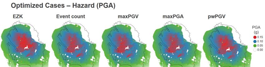
B.2       Mathematical Notation and Definitions ............................................................................... 86
   B.3       Uniformly Sampling from a Convex Polyhedron ................................................................... 87
   B.4       Sampling strategy for calibration of the Random Forest proxy model................................. 88
Appendix C Comparison of 2018 results with the 2017 optimisation study ........................................ 90
   C.1       V4 to V5 differences .............................................................................................................. 90
   C.2       Comparing Random Forest analysis between V4 and V5 ..................................................... 95
Appendix D List of Abbreviations .......................................................................................................... 97

                                                               Page 5 of 98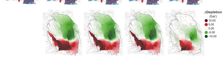
Page 6 of 98
1 Introduction
1.1 Study background
2014 Instemmingsbesluit

Following Winningsplan 2013, the Minister of Economic Affairs decided to restrict production from
the five production clusters in the Loppersum area to 3 Bcm/year. In subsequent decisions by the
Minister and upon appeal at the Raad van State, this volume was further reduced until these cluster
were fully closed-in. In effect this was the first intervention and optimisation of the distribution of the
gas production in relation to seismicity over the Groningen field.

Winningsplan 2016

In the first quarter of 2016, the first systematic approach to optimisation of the distribution of the
production from the clusters in the Groningen field to reduce seismicity was carried out. This was
reported in the Technical Addendum to the Winningsplan submitted on 1/4/2016, Reference [1]. This
initial optimisation was based both on mathematical optimisation and on a practical understanding of
the pressure response of the reservoir to the distribution of the production and the impact on the
resulting seismicity. The impact of the alternative distribution of production on the seismicity and risk
was checked by performing dedicated hazard and risk assessments.

2017 Production Optimisation study

In Article 3.2 of the 30/9/2016 Instemmingsbesluit for NAM’s Winningsplan 2016, Reference [2], and
of the subsequent 24/5/2017 Wijzigingsbesluit, Reference [3], NAM was tasked by the Minister of
Economic Affairs to investigate whether an alternative distribution of production from the Groningen
field could reduce the seismic hazard or risk. NAM embarked on a detailed optimisation study, and
issued a final report to SodM on 27/11/2017, Reference [4].

        Fragment from the 30/9/2016 Instemmingsbesluit Article 3.2

SodM approval and request for update

In a letter to NAM on 30/11/2017, Reference [5], SodM informed NAM that the optimisation study
had been executed to the satisfaction of the Inspecteur Generaal der Mijnen and could be issued to
the Minister. SodM described the scientific quality of this study as “state-of-the-art”. However, SodM
did not yet make a judgement on the applicability of the study and referred to its earlier reservations
as stated in its reaction to the “Plan van Aanpak”, Reference [6], that the limitations of the underlying
seismological model will affect the optimisation of production.

On 20/2/2018, SodM informed NAM by letter that the optimised production distribution could not be
implemented in the field, because the underlying seismological model was deemed inadequate,

                                                  Page 7 of 98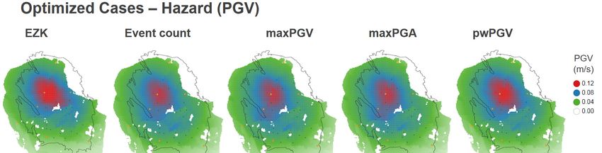
Reference [7]. SodM requested for an update of the study within 6 months, using the V5 update of
the seismological model which had meanwhile become available. This V5 update presented a better
areal match of the historic earthquakes (as compared to the previously used V4 seismological model).

Basispad Kabinet

On 29/3/2018 the Minister of Economic Affairs sent a letter to Parliament, Reference [8], announcing
the ambition of the cabinet to reduce the production from the Groningen field as soon as possible,
leading to cessation of production around 2030. The letter contained a scenario of annual production
volumes for the period 2018-2031 labelled “Basispad Kabinet”.

Following these developments for the Groningen production outlook, NAM agreed with SodM to base
the requested update of the production optimisation study on the new production scenario “Basispad
Kabinet”.

1.2 Study objective
The Groningen field has 22 production locations (20 clusters and two satellites) by which gas can be
produced from the field (Figure 1-1). All wells are typically drilled vertically, and hence extract gas
from a small area directly underneath the cluster area. The only exception is the deviated well, EKL-
13, that is producing gas from the reservoir at some distance from the other (vertical) wells of the
Eemskanaal cluster. All these clusters can be controlled relatively independently within their
respective operational constraints. This offers the opportunity to make choices in how production is
spatially distributed over the field. It can be observed from Figure 1-1 that the historical earthquakes
display some degree of spatial clustering as well.

In line with Article 3.2 of the Instemmingsbesluit, this study aims to establish the optimal distribution
of production across the various production clusters to minimise seismic hazard or risk, for a given
total field offtake profile.

                                              Page 8 of 98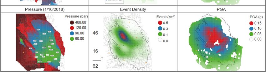
Production cluster                                          Earthquakes (M≥1.5)
                                                                           1/1/1995 to 27/8/2018

Figure 1-1      Hazard (earthquakes) and controls (production clusters)

1.3 Report structure
The structure of the study is described in chapter 2, and the hazard and risk (HRA) model in chapter 3.
In chapter 4 the optimisation is discussed based on simplified assumptions for the production clusters.
In this way the theoretical optima are established for different objective functions.

Chapter 5 describes the fitting of a proxy (Random Forest) model to the optimisation results, allowing
for further understanding of the behaviour of the HRA model (in addition to the optimal production
fractions).

Chapter 6 described how subsequently the theoretical optimum production distributions are rerun
using the subsurface model coupled with a high-fidelity surface network model which reflects the
operation limitations of the surface facilities, allowing for more realistic implementation of production
distributions. These “operationalised” production optimisations are evaluated using the full logic-tree
in order to establish the expected numbers of buildings that exceed the Meijdam norm.

                                                  Page 9 of 98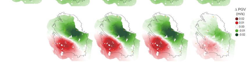
2 Study setup
2.1 Production induced seismicity cause and effect chain
Production induced seismicity and its effects at surface are modelled according to the following cause
and effect chain (Reference [9]):

              Production from clusters

                       Pressure depletion

                                 Compaction

                                       Event Rate (Earthquakes)

                                               Hazard

                                                        Risk

2.2 Model implementation
In the Hazard and Risk Assessments issued by NAM, the first step in the cause and effect chain up to
“Pressure depletion” are calculated in the dynamic reservoir simulator (Mores, part of the Dynamo
tool suite1), as described in Reference [10]. The subsequent calculation steps to predict earthquakes,
hazard, and/or risk, are calculated in the seismic Hazard and Risk Assessment (HRA) model as
described in References [11] and [12].

This model representation of the cause and effect chain can be implemented within a control loop,
which allows for a model-driven optimisation. A high-level overview of the calculation steps is
depicted in Figure 2-1 :

       1) Optimisation algorithms, which are part of the Dynamo tool-suite, are driving the process. The
          total required production from the field is distributed across the production clusters (model
          controls) according to an initial distribution, which is issued from the optimiser to the Mores
          reservoir simulator.
       2) In Mores, the response of the reservoir to the imposed distribution of gas offtake is calculated
          in terms of reservoir pressures, and provided to the HRA model.
       3) Within the HRA model the rock compaction due to the pressure depletion is calculated. As a
          function of the compaction in time (yearly steps), spatial estimates are generated for events,
          hazard and risk.
       4) This output is subsequently imported back into Dynamo and (a selection thereof is) used
          during the optimisation.

1
    Shell proprietary software

                                               Page 10 of 98
Figure 2-1 Modelling workflow
2.3 Model controls
As described in section 1.2, in principle each one of the 22 production cluster locations across the
Groningen field can be controlled relatively independently within their respective operational
constraints, and hence act as an independent model control for the optimisation. However, to keep
the calculation times of the modelling effort within somewhat reasonable bounds, a certain degree of
“lumping” was done of the individual production clusters to reduce the number of model controls.
This lumping was done to ensure compatibility of this study with the June 2018 Addendum to the
Hazard and Risk Assessment – November 2017, Reference [13], that was requested by the Ministry of
Economic Affairs. In the request, Reference [14], NAM was asked to comply with the advice by SodM
following the Zeerijp earthquake, Reference [15]. The SodM advice specified amended production
regions2 for which production fluctuations should be limited. To both accommodate this request, and
the request to optimise the production distribution, NAM implemented a production cluster start-up
list in its modelling effort, Table 2-1.
2
The “East” region as stipulated in the Instemmingsbesluit, Reference [2], was broken up into 3: Bierum, East-
Central (Amsweer, Tjuchem, Schaapbulten, Siddeburen, Oudeweg) and South-East (Zuiderpolder,
Scheemderzwaag and De Eeker).
Page 11 of 98Start-up Priority Region Clusters
1 North BIR (constant rate)
2 Eemskanaal EKL (constant rate, winter only)
3 South-East ZPD/SZW/EKR
4 East-Central (1) OWG/SCB
5 South-West (1) ZVN/SPI
6 East-Central (2) AMR/TJM/SDB
7 South-West (2) SAP/TUS
8 South-West (3) KPD/SLO/FRB
Table 2-1 Production start-up list. Starting from the top of this list, groups of clusters are sequentially opened-up by the
surface network model until the total required production can be achieved. Source: Reference [13]
These same regions are used for this report into the optimisation of production distribution. This
implementation means a slight update with respect to the 2017 study (depicted in Figure 2-2):
• The former [East] and [Siddeburen] controls were redefined to improve the resolution
around Appingedam.
• The former [South-Central] control was split into 2 regions to better honour geology.
• Production clusters ‘t Zandt and Leermens were previously (2017) dedicated controls, but
these are now lumped into a single control [ZND_LRM].
Figure 2-2 Model controls for this study update (2018 Production Optimisation) versus the 2017 Production
Optimisation. The production clusters in the right-hand panel are colour-coded in line with the Ministerial
regions as defined in Reference [14].
Page 12 of 982.4 Objective functions
2.4.1 Practicability of a risk-based optimisation
From previous experience, it is known that a typical optimisation comprises about 250 individual
simulations over 15 outer iterations. Although the dependence of risk on hazard is well understood
and modelled, it cannot be distilled into a simple correlation without sacrificing accuracy and
applicability. On the other hand, the risk logic-tree is considerably larger than the hazard one (as
described in section 3.4.1, the risk logic-tree has 216 branches compared to 24 in the hazard one), and
each risk simulation requires significantly more time to run (roughly 50% - 100% increase in run-time).
Taken together, these observations render it impossible to perform a risk-based optimisation within
a reasonable time-frame while maintaining a sufficient level of accuracy. For this reason, a hazard-
based optimisation approach (with a risk-assessment of the optimised distribution) was followed. The
HRA model calculates several hazard-based “HRA metrics”, which, separately or together, can be
assigned as the objective function for the optimiser.
The objective functions used in this study are based on:
• Nuisance: Event Count
• Hazard: Maximum PGA (Return period of 475 y)3, Maximum PGV (Return period of 475 y) 4
• Risk: Population weighted PGV5
2.4.2 Event Count
The Event Count is a cumulative over the entire field, and, as such, represents the impact of a certain
production scenario on the entire field.
2.4.3 Maximum Peak Ground Acceleration (maxPGA) and Peak Ground Velocity
(maxPGV)
The Hazard objectives (maxPGA and maxPGV) are established as the highest recorded value on the
hazard map associated with a certain production scenario. As such, these do not provide a response
across the entire system, other than that no other place in the field is modelled to experience a hazard
that is higher than this value. Focus of the optimisation based on these objective functions is the high
seismic region around Loppersum.
2.4.4 Population weighted PGV (pwPGV)
The population-weighted PGV was chosen as a proxy for total population risk. This is based on
analogy with the PAGER effort in USGS6, which provides a rapid assessment of the impact of
earthquakes (in terms of fatalities and economic loss) and estimates the population exposed to
different levels of shaking.
In the PAGER method, the Modified Mercalli Intensity scale (MMI) is used to represent ground shaking
combining both observations and measurements. Where measurements are available PGA and PGV
are converted to MMI. The paper by Wald et al, Reference [16], shows that PGV correlates with a
wider range of macro-seismic intensities, whereas PGA saturates at higher levels of MMI. Once the
3
PGA hazard is generated for the 475-year return period for all surface locations.
4
PGV hazard is generated for the 475-year return period for all surface locations.
5
A weighted average PGV is calculated using the population at each location as the weight
6
https://earthquake.usgs.gov/data/pager
Page 13 of 98population within different bands of shaking has been calculated, empirical vulnerability functions are
used to estimate the losses, Reference [17]. Furthermore, the paper by Allen et al, Reference [18],
states that earthquake mortality appears to be systematically linked to the population exposed to
severe ground shaking (MMI VIII+, which would be PGV values above 0.30 m/s according to Wald et
al. (1999)). The population weighted PGV again reflects a response of the entire system, it is calculated
by multiplying each cell of the hazard map with the population in that location.
The population density is given in Figure 2-3.
Figure 2-3 Population map in relation to the Groningen gas field (log scale)
2.5 Boundary conditions
The following boundary conditions were imposed for the optimisation:
2.5.1 Production profile
The total field production as used for this study was taken as per the production profile “Basispad
Kabinet” for average temperature, Figure 2-4, which was received by NAM from the Ministry of
Economic Affairs on 2/5/2018, Reference [14]. Note that this production profile is slightly different
compared to the 29/3/2018 profile as mentioned in section 1.1, Reference [8].
The optimisation window is for this production scenario limited to 4 years, from 1/10/2018 to
1/10/2022. Hence the (relatively) low production volumes from gas-year 2022/2023 onwards are
excluded from the optimisation. These years follow the onstream date of the additional nitrogen
plant. For these low production-volumes, the pressure equilibration between the northern and
southern areas of the field will dominate the seismic response, masking the effect of the production
controls.
Page 14 of 98For the optimisation and data driven analysis, a flat production profile throughout the production year
is assumed (no seasonal fluctuation). For the operationalisation and risk calculations the monthly
production variations as specified in Reference [14] are included.
Figure 2-4 Production profile “Basispad Kabinet” for average temperatures, as received by NAM from the Ministry
of Economic Affairs on 2/5/2018. The optimisation window is highlighted (1/10/2018 to 30/9/2022).
2.5.2 Production fractions
Within the production profile, the production fractions of the various model controls were kept
constant, an example is given in Figure 2-5.
Figure 2-5 Break-down of optimisation production profile by control
2.5.3 Optimiser
• The optimiser is allowed full freedom in the requested production from each control, clusters
are allowed to produce anything between 0 and their full capacity.
• The optimiser is allowed to vary all controls in order to minimise the objective (although the
Loppersum clusters were set to zero during the optimisation runs to limit the calculation
effort).
Page 15 of 98• The maximum cluster capacity is imposed by means of a simple fixed THP constraint, providing
a first order reflection of the currently installed compressor capacities.
• There are no additional constraints imposed to reflect the surface facilities (e.g. pressure
losses in the Groningen pipeline ring).
• A simple cluster uptime assumption of 90% to reflect planned and un-planned downtime was
used.
2.6 Subset of uncertainty tree
The epistemic uncertainty in the hazard and risk model is captured in a logic tree (section 3.4). The
2017 optimisation study showed there is a highly congruous behaviour between the various branches
of the Hazard uncertainty tree, Reference [4]. Given the time pressure on this study update and
stretched calculation resources, it was decided to limit this study update to 5 branches out of the total
24 branches comprising the hazard logic-tree. The five branches were selected to reflect the full
spread of the hazard logic-tree (Figure 2-6). The following branches have been used:
• Branch 22 = U_3_2
• Branch 24 = U_4_2
• Branch 6 = C_3_2
• Branch 9 = L_1_1
• Branch 14 = L_3_2
In chapter 5 the results for these branches are reviewed to establish the representativeness of this
subset versus the potential need to evaluate additional branches.
Figure 2-6 Selected subset of branches from the Hazard logic tree
Page 16 of 983 Hazard and Risk Model
This study update utilises the V5 Hazard and Risk Model. This is the same HRA models as used in the
HRA assessment of the Basispad Kabinet production scenario, Reference [13].
3.1 Dynamic reservoir simulation model
The dynamic response of the reservoir to the choices in production distribution across the various
production clusters are modelled with the dynamic reservoir model. For the 2017 optimisation study
the V4 Mores model was used, Reference [10], whereas this study update utilises the V5 Mores model.
A full description of model V5 and the main changes with respect to V4 are given in Reference [19].
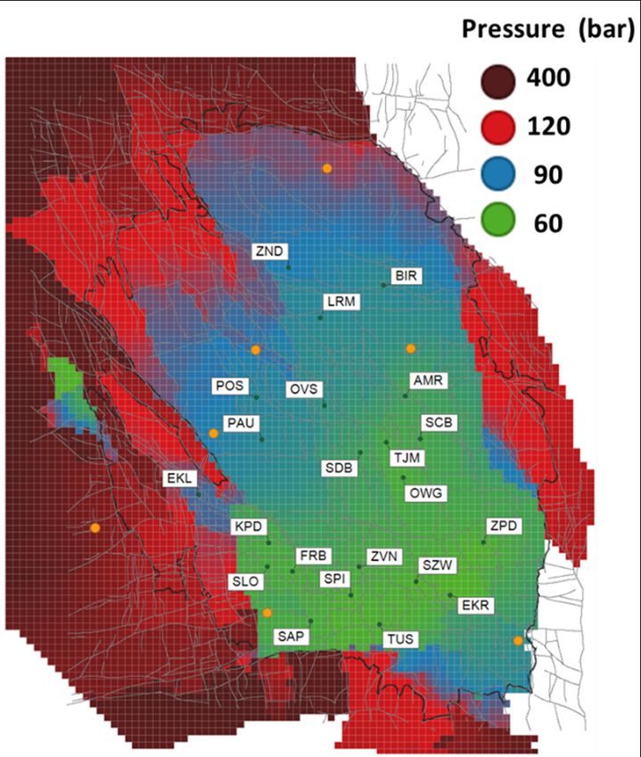
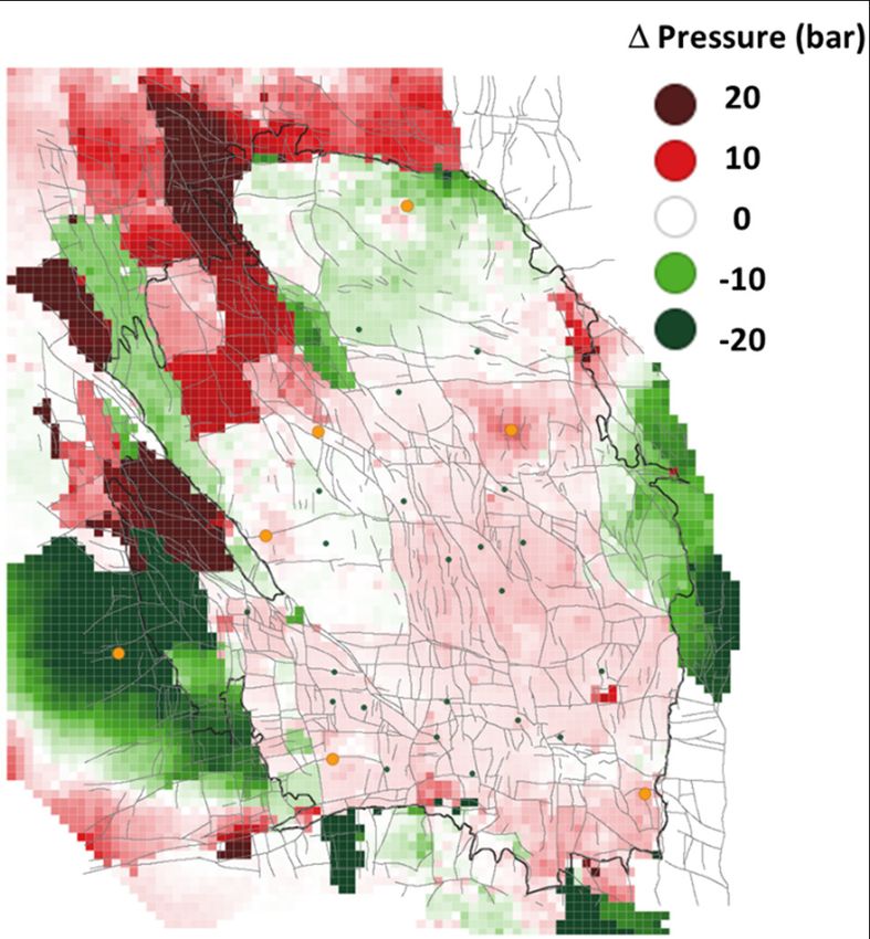
The history matched pressure in 2018 and differences between V4 and V5 models are shown in Figure
3-2. The most prominent changes for the pressure match resulted from a shift in focus towards the
(high resolution) CITHP-to-CIBHP data, to better capture production induced transient effects that
were induced by the Ministerial production caps.:
• The connectivity between the Ten Post, De Paauwen and Overschildt production clusters was
reduced, aligned with the large fault (125 meter throw) in between these production clusters.
A fault seal factor multiplier was assigned to this fault in the history matching process.
• From CITHP data it was observed that there is a 3-5 bar pressure lag within the Southwestern
area of the field between West (clusters Kooipolder, Slochteren, Froombosch and Sappemeer)
and East (clusters Spitsbergen and Tusschenklappen). These two areas are separated by a
series of relatively large faults (>100m throw) which to the North are associated with the pop-
up blocks. To reproduce this pressure lag in the reservoir model, additional fault seal factors
had to be applied.
• The RFT data acquired in 1998 from the Rodewold-1 well (Southwestern periphery) showed
depletion. In the V4 history match a depletion path was implemented via the graben
separating the northwest from the southwest periphery. The V5 model utilises an alternative
depletion path to establish a pressure match. Depletion is implemented along the horst block
via Ten Boer towards Eemskanaal.
Page 17 of 98Figure 3-1 Biggest dynamic changes between Mores model V4 and V5. Faults that were made more sealing indicated by
red arrows, alternative depletion paths in southwestern periphery indicated by red and orange arrows.
Page 18 of 98Figure 3-2 History matched pressure using V5 Mores model at 1st January 2018 and differences w.r.t. V4 model at the
same time.
3.2 Seismological model
For this study, the V5 seismological model was used as described in References [11] and [12].
3.3 Ground-Motion-Prediction Equation
As part of the V4 to V5 update of the HRA model, the Ground-Motion-Prediction Equation did see
some material changes. Up to Base North Sea the GMPE is more or less the same, but the amplification
factors governing the propagation of the seismic energy between the Base North Sea and surface were
updated.
Figure 3-4 shows the difference between the PGA maps for the Base North Sea and the surface for
both the V4 and the V5 model over a period of 5 years for the 21.6 Bcm production scenario. It can be
observed that the V4 model calculates a somewhat uniform increase in PGA as the seismic energy
travels through the shallower subsurface, whereas the V5 model shows a dampening in the
Loppersum and Southwestern area of the field and a strengthening in the East.
Although the GMPE is a highly intricate calculation and as such it is not possible to extrapolate
observations from a single production scenario, Figure 3-4 does show that there are significant
differences between the V4 and V5 model.
Page 19 of 98Figure 3-3 Schematic illustration of the HRA model layers
V4 V5
Figure 3-4 Net difference in PGA between Base North Sea and surface for V4 and V5 HRA model, over the period
1/1/2017 to 1/1/2022 for a 21.6 N.Bcm offtake.
Page 20 of 983.4 Model uncertainty
There are two levels of uncertainty in the model results:
• Aleatory uncertainty
Aleatory uncertainty is the result of the natural randomness in a process. Given the stochastic
nature of the HRA simulation, how big should the reduction in the various metrics be for these
to be larger than the stochastic variability of the results? For a given choice of metric and initial
condition, this applies to each of the optimisation runs.
• Epistemic uncertainty
Epistemic uncertainty is the scientific uncertainty in the model of the process. It is due to
limited data and knowledge. The epistemic uncertainty is characterised by alternative models,
which were captured in a logic tree. Since it is not known which of the 24 logic-tree branches
reflects the field reality, how do the gains due to optimisation compare to the alternative HRA
model’s represented by different branches of the logic tree?
3.4.1 Epistemic uncertainty
In the HRA model, it is assumed that the uncertainty in the reservoir pressure is smaller than the
uncertainty in other parameters and hence it was not explicitly included as an uncertainty in the logic
tree. To reflect that pressure cannot be measured outside of well control, a spatial smoothing step is
applied.
Within the HRA model the epistemic uncertainty is captured by means of an uncertainty tree. The V5
vintage of the HRA model involves a logic-tree for Hazard with 24 branches, and for Risk of 216
branches.
The logic tree for the hazard assessment comprises three sets of branches to capture the uncertainty
in the most uncertain elements, Figure 3-5. The first branches cover the uncertainty with respect to
Mmax in the seismological model, and the second and third sets capture the uncertainty related to the
GMPE (tau and sigma). Each branch of the logic tree represents a scenario, and by combining all
scenarios using the weights in the logic tree, the mean hazard map can be calculated.
Figure 3-5 Hazard logic tree.
Page 21 of 983.4.2 Aleatoric uncertainty
Especially the Monte Carlo setup of the HRA model introduces an aleatoric model variability (also
referred to as statistical or stochastic uncertainty).
The approach taken to address the stochastic variability works as follows. For each branch of the logic-
tree, the HRA model was run multiple times, using fixed control settings, a fixed grid size, and a fixed
number of Monte Carlo draws (‘catalogue size’). Each time the seed value for the random-number
generator was varied. The resulting set of values was then used to validate stability of the estimated
hazard and risk metrics. An example is given in Table 3-1. The aleatoric uncertainty within the HRA
model was found to be typically around 1-2%.
Table 3-1 Aleatoric uncertainty in the HRA model as tested for branch 6 using 10 different random seeds
3.5 Model robustness
In line with section 3.4 the model robustness was assessed.
3.5.1 Robustness with respect to aleatoric uncertainty
Each run of the HRA model is performed on an observation grid (with user-supplied spacing) and
involves the sampling of probability distributions for the various HRA model parameters. Using finer
grids and increased sampling will result in better estimation of the outcome (i.e. smaller confidence
intervals), but also consumes more computational resources and consequently slows down the
optimisation process. The execution time is roughly linear in the number of draws and quadratic in
terms of the grid-size. It is, therefore, necessary to strike a balance between accuracy and overall
computational time.
To this end, a number of production scenarios were tested:
• Production fractions based on 2017 actual data
• Production fraction as used in the HRA calculation for Basispad Kabinet (GY 18/19)
• Minimisation of number of Events (earthquakes)
• Minimisation of maximum Peak Ground Acceleration
• Minimisation of population weighted Peak Ground Velocity
Each of these production scenarios were simulated for varying resolutions of the sampling grid:
• 250m
• 500m
• 1000m
• 1500m
Page 22 of 98And for a varying number of Monte Carlo draws (catalogue size):
• 50,000
• 75,000
• 100,000
• 150,000
• 200,000
The associated model results are summarised in Figure 3-6.
Event count maxPGV
maxPGA pwPGV
Figure 3-6 Robustness assessment for varying grid resolution and catalogue size
The Event count is hardly affected by the choices in grid resolution and catalogue size.
The pwPGV metric is obviously affected by the gridsize (number of people per gridblock varies), but
between the various gridsizes there are no differences in the order of the scenarios.
From Figure 3-6, it can be concluded that there are no big differences between 250 and 500m
resolution, but at 1000 and 1500m differences start showing with respect to the 250m reference.
Consequently, the 500m grid was selected. At this grid resolution, a catalogue size of 75,000 yields
Page 23 of 98stable results. An overview of the numerical performance is given in Table 3-2. For the selected
numerical settings the associated runtime for the HRA model is approximately 1:45 hr7.
Table 3-2 Model calculation times as a function of grid resolution and catalogue size
3.5.2 Robustness with respect to epistemic uncertainty
Qualitative assessment of the robustness with respect to epistemic uncertainty is somewhat more
complicated and was done by running the HRA simulation for the full logic-tree and comparing it to a
reference case. A somewhat more rigorous approach to the assurance of robustness with respect to
the epistemic uncertainty is to calculate, for each of the optimisation results, the expected value of
optimisation metric. To ensure that the results are optimised with respect to the entire uncertainty
range as captured in the logic tree, a dedicated optimisation is run for each of the uncertainty-tree
branches, using the following process (Figure 3-8):
• First the objective function and initial production distribution is selected
• The following steps are executed in parallel for each branch of the logic tree
o Given the selected set of objective function and initial rate, a dedicated SPMI
optimisation is run,
o An optimum production distribution is obtained,
o The optimisations’ end results are each evaluated on the entire logic tree (24 branches)
and the value of the logic-tree mean is calculated for each metric using the weights of the
various branches
After running the full uncertainty-tree on the optimal distributions obtained for each branch and
weighting the resulting metric values by the probabilities associated with each branch, the optimal
distribution (lowest expected value for the optimisation metric) is selected.
This process setup ensures a consistent hazard assessment (i.e. taking into account the epistemic
uncertainties) and enables a like-for-like comparison of the optimisation outcomes’ performance for
each branch. The comparison is done for both PGA and PGV differences. Figure 3-7 shows an example
of the areal PGA, along with uniform hazard spectra at specific locations (e.g. Groningen, Loppersum,
Ten Boer, etc.), where two scenarios are compared. Although the epistemic confidence intervals do
still overlap, there is a significant reduction of hazard in Delfzil and Loppersum.
7
Note that solely for the optimisation purpose these settings are excessively strict. The optimisation would only
require the model response to production changes to be stable within limits. So the model used for optimisation
does not need to delivery accurate hazard and risk metrics only changes to these metrics with the correct sign
under production changes. Having these tight settings does however allow for a more quantitative comparison
with previous HRA analyses.
Page 24 of 98Figure 3-7 Sample HRA output visualisation showing the PGA map for the EZK reference case (see section 6.3.2) along with uniform hazard spectra for the reference case with a comparison
to an optimised case (event count) for selected locations. The reference and optimised scenarios are plotted in red and blue respectively, with shaded area representing the
epistemic uncertainty The PGA map shows the acceleration at 0.01s.
Page 25 of 98Figure 3-8 Optimisation process-flow for an optimisation metric/initial distribution pair
Page 26 of 984 Optimisation
4.1 Setup
4.1.1 Controls
To reduce the calculation time, only 8 out of the 10 controls (section 2.1) were used in the optimisation
runs. The two controls within the Loppersum region were excluded, and their production fractions
were set to zero in all runs:
• [ZND_LRM] = 0
• [PAU_POS_OVS] = 0
The validity of this assumption is cross-checked and validated in chapter 5.
4.1.2 Reference Case
The actual production split as of calendar year 2017 was used as the reference case and as the initial
starting point for the optimisation.
Control Production fraction
1 [BIR] 0.11
2 [EKL] 0.02
3 [AMR_TJM_SDB] 0.29
4 [OWG_SCB] 0.12
5 [EKR_SZW_ZPD] 0.20
6 [FRB_KPD_SLO] 0.13
7 [SAP_TUS] 0.05
8 [ZVN_SPI] 0.08
Sub total 1.00
9 [ZND_LRM] 0.00
10 [PAU_POS_OVS] 0.00
Table 4-1 Production and production fractions of the reference case (calendar year 2017) by model control
4.1.3 Optimisation window
A four-year optimisation window was used, to avoid “noise” from pressure equilibration effects once
field offtake drops significantly (after nitrogen plant comes on-stream).
4.2 Results
In Table 4-2 to Table 4-5 the optimised production fractions are given for the various optimisation
objectives. Per objective function, a dedicated optimisation was executed on each of the selected
branches of the uncertainty tree. Each set of optimised fractions were then evaluated across the entire
logic tree (24 branches) to yield the logic tree mean. The branch that yielded the best result for the
logic tree mean for a given objective function is highlighted in bold. For reference, the initial rates for
the optimisation are included, named “branch 0”. These are the actual production fractions as per
calendar year 2017.
Page 27 of 98Events
Branch Itr Case BIR EKL AMR_TJM_SDB OWG_SCB EKR_SZW_ZPD FRB_KPD_SLO SAP_TUS ZVN_SPI
0 CY 2017 actual 0.11 0.02 0.29 0.12 0.19 0.13 0.05 0.08
6 8 7 - - - - 0.32 0.27 0.12 0.29
9 10 5 - - - 0.06 0.32 0.19 0.15 0.29
14 10 5 - - - 0.06 0.32 0.19 0.15 0.29
22 7 18 - - - - 0.30 0.28 0.13 0.30
24 7 18 - - - - 0.30 0.28 0.13 0.30
Table 4-2 Production fraction for each control across the various branches when optimised for Events
maxPGA
Branch Itr Case BIR EKL AMR_TJM_SDB OWG_SCB EKR_SZW_ZPD FRB_KPD_SLO SAP_TUS ZVN_SPI
0 CY 2017 actual 0.11 0.02 0.29 0.12 0.19 0.13 0.05 0.08
6 9 5 - 0.22 - 0.14 0.27 0.19 0.08 0.10
9 8 5 - 0.01 - 0.23 0.34 0.29 0.13 -
14 5 11 - 0.01 - 0.24 0.36 0.27 0.12 -
22 7 12 0.01 0.17 - 0.14 0.35 0.23 - 0.11
24 7 1 0.04 0.22 - 0.15 0.22 0.16 0.09 0.12
Table 4-3 Production fraction for each control across the various branches when optimised for maxPGA.
maxPGV
Branch Itr Case BIR EKL AMR_TJM_SDB OWG_SCB EKR_SZW_ZPD FRB_KPD_SLO SAP_TUS ZVN_SPI
0 CY 2017 actual 0.11 0.02 0.29 0.12 0.19 0.13 0.05 0.08
6 7 15 - 0.03 - 0.16 0.24 0.23 0.09 0.25
9 5 16 - - - 0.16 0.25 0.21 0.11 0.27
14 6 5 0.01 0.08 - 0.15 0.25 0.19 0.11 0.20
22 8 12 - - 0.01 0.16 0.23 0.22 0.16 0.23
24 7 8 - 0.01 - 0.22 0.23 0.23 0.09 0.22
Table 4-4 Production fraction for each control across the various branches when optimised for maxPGV
pwPGV
Branch Itr Case BIR EKL AMR_TJM_SDB OWG_SCB EKR_SZW_ZPD FRB_KPD_SLO SAP_TUS ZVN_SPI
0 CY 2017 actual 0.11 0.02 0.29 0.12 0.19 0.13 0.05 0.08
6 2 14 0.06 0.01 0.18 0.07 0.25 0.08 0.03 0.31
9 10 10 0.19 - 0.11 0.23 0.36 - 0.11 -
14 8 17 0.19 - - 0.29 0.39 - 0.13 -
22 2 7 0.07 0.01 0.20 0.24 0.29 0.09 0.04 0.06
24 10 5 - - - 0.31 0.32 0.13 0.13 0.11
Table 4-5 Production fraction for each control across the various branches when optimised for pwPGV.
The results for the various optimisations are summarised in Figure 4-1, where the optimum production
fraction is given for each control. It can be observed that only the pwPGV optimisation is utilizing the
[BIR] control, and only the maxPGA optimisation is utilizing the [EKL] control. None of the
optimisations are using the [AMR_TJM_SDB] control. The remaining controls are utilised to varying
degrees by the different optimisations. Event count optimisation is exclusively producing from the
South, while pwPGV optimisation avoids the more populated South-West by not utilizing the
[FRB_KPD_SLO] and [ZVN_SPI] controls.
Page 28 of 98Figure 4-1 Optimised production fractions of the controls for the different optimisation objective functions
The improvements in hazard metrics are given in Table 4-6. These results are derived from the logic
tree mean, i.e. the production fractions in Figure 4-1 evaluated across all 24 logic tree branches. The
improvements vary between 5 and 14 percent depending on the metric that is optimised based on
the objective function.
Objective Hazard Metric Improvement
Events maxPGA maxPGV pwPGV Events maxPGA maxPGV pwPGV
Reference (2017 Act) 62.4 0.155 0.127 0.039
Event Count 58.7 0.149 0.123 0.037 -6% -4% -3% -5%
maxPGA 56.3 0.140 0.112 0.040 -10% -10% -12% 2%
maxPGV 56.0 0.150 0.112 0.039 -10% -3% -12% -1%
pwPGV 53.6 0.152 0.110 0.039 -14% -2% -13% 0%
Table 4-6 Optimisation results with respect to the HRA metrics
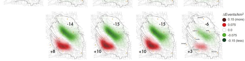
In Figure 4-2 to Figure 4-6 the optimisation results are given in map view. In Figure 4-2 the reference
case is displayed. The bottom left-hand panel gives the starting point for the optimisation: the
reservoir pressure at 1/10/2018. The production fractions for the reference case (Table 4-1) are
displayed as a bubble map in the top centre panel. The resulting depletion over the four-year
optimisation period (1/10/2018 to 1/10/2022) is given in the top left-hand panel, and the associated
event density in the bottom centre panel (in total, there are some 46 events expected in the North of
the field, and 16 in the South). The subsequent PGA and PGV maps are in the left-hand side of the
panel. For reference, the fault pattern is displayed in the background. Additionally, the main cities are
highlighted as orange dots (labelled in the top right-hand panel), and the production clusters as black
dots (labelled in the bottom right-hand panel).
Page 29 of 98This same visualisation panel was used to present the optimisation results for the various objective
functions, but now the differences are displayed with respect to the reference case. Table 4-3 gives
the results for the Event count optimisation. Note that the production fraction bubble map highlights
the optimised production fractions in red, with the reference case production fractions kept in blue.
All production is moved towards the southernmost 4 controls. As a result, the depletion has increased
in the South (compared to the reference case) and reduced in the North. In terms of absolute
depletion (top left-hand panel), there is even some pressure rebound just south of the city of Delfzijl.
In total a reduction of some 9 events is expected as compared to the 62 events in the reference case.
This constitutes of a reduction of 16 in the North, and an increase of 7 in the South. The net effect in
terms of PGA and PGV gives an almost horizontal divide between increase and reduction with respect
to the reference case (right-hand panel).
The optimisation with respect to maxPGA utilises the [EKL] and [OWG_SCB] controls, resulting in
increased hazard in the South-West, rotating the net hazard effect by some 45o.
The maxPGV optimisation does not utilise the [EKL] control, with more offtake from the central
controls in the South,[ZNV_SPI] and [SAP_TUS]. This makes the net gain with respect to the reference
case similar to the Event count optimisation, although less pronounced both in terms of event count
and hazard. The net reduction in Event count has reduced to 6 (North: -12, South: + 6).
The population weighted PGV optimisation yields the biggest areal reduction in PGA and PGV
including the entire South-West, although the magnitude of reduction is somewhat modest compared
to the other optimisation strategies. This is achieved by opening up the Northern-most [BIR] control
and not utilizing controls in the South-West that are close to the city of Groningen. The net reduction
in events is also less than in the other strategies (+2 in the South and -6 in the North).
Page 30 of 98Figure 4-2 Optimisation reference case – production distribution and subsequent impact on pressure, event density and hazard
Page 31 of 98Figure 4-3 Optimisation for Event count – Changes with respect to reference case (Figure 4-2) in terms of production distribution and subsequent impact on pressure, event density and
hazard. The relative reduction in event count and maximum values of PGA and PGV are summarised in Table 4-6.
Page 32 of 98Figure 4-4 Optimisation for maxPGA – Changes with respect to reference case (Figure 4-2) in terms of production distribution and subsequent impact on pressure, event density and
hazard. The relative reduction in event count and maximum values of PGA and PGV are summarised in Table 4-6.
Page 33 of 98Figure 4-5 Optimisation for maxPGV – Changes with respect to reference case (Figure 4-2) in terms of production distribution and subsequent impact on pressure, event density and
hazard. The relative reduction in event count and maximum values of PGA and PGV are summarised in Table 4-6.
Page 34 of 98Figure 4-6 Optimisation for pwPGV – Changes with respect to reference case (Figure 4-2) in terms of production distribution and subsequent impact on pressure, event density and
hazard. The relative reduction in event count and maximum values of PGA and PGV are summarised in Table 4-6.
Page 35 of 985 Data driven analysis of model response
5.1 Random Forest proxy models
To further complement the understanding of the behaviour of the HRA model (rather than to only
state the optimal production fractions), the complex HRA model was approximated with a simpler but
still reasonably accurate proxy model that can be analysed more directly using experimental design
type techniques, e.g. variable importance plots and partial dependence plots. The chosen class of
proxy models are Random Forests. Although other models may have worked equally well, Random
Forests have the following features that contribute to their particular utility in this case:
• Can capture non-linear effects and interactions between controls
• Good out-of-box performance without tuning of algorithm parameters
• Computational efficiency
• Diagnostic tools that allow to extract information like variable importance and partial
dependence of model response on a subset of controls.
A detailed description of the underlying theory and further references are provided in Appendix A.
Dedicated Random Forest proxy models were built for each combination of branch and objective
function, that can mimic the relation between model input (controls setting) and model output
(optimisation metric), to be analysed further.
5.2 Sampling of the control space
To fit the Random Forest models, the control space8 had to be sufficiently sampled. A detailed
description of the sampling strategy is given in Appendix B. Table 5-1 summarises the applied
boundary conditions.
control production fraction control production fraction
BIR 0.01 ≤ ci ≤ 0.25 FRB_KPD_SLO 0.01 ≤ ci ≤ 0.35
EKL 0.01 ≤ ci ≤ 0.25 SAP_TUS 0.01 ≤ ci ≤ 0.16
AMR_TJM_SDB 0.01 ≤ ci ≤ 0.51 ZVN_SPI 0.01 ≤ ci ≤ 0.30
OWG_SCB 0.01 ≤ ci ≤ 0.31 ZND_LRM 0.01 ≤ ci ≤ 0.36
EKR_SZW_ZPD 0.01 ≤ ci ≤ 0.38 PAU_POS_OVS 0.01 ≤ ci ≤ 0.60
Table 5-1 Sampling space for control fraction of each control
Even though constraints were already applied on the to ensure that (most of the) combinations
would achieve the minimal production threshold, some of the more extreme combinations can still
drop out. To fit the proxy models, only samples were considered that have at least an average
production ≥15.675 Bcm/year (0.2 Bcm deviation). When applying ±0.2 Bcm deviation on total
optimisation window (i.e. ±0.05 Bcm deviation annually) instead of annually 4,227 versus 4,366
samples passed the filtering rule
(on averaged over the forecasting period production volume). Limited impact when applying stricter
production threshold was observed.
8
The control space is span by all possible combinations of production fractions for the various controls (the
(lumped) production clusters)
Page 36 of 985.3 Overall model quality assessment
Random Forest models were trained on the filtered sample sets and the quality of each model is
assessed using blind testing.
As shown in Table 5-2, it was established that the normalised RMSE (defined as the root mean squared
error of the model normalised by the mean response of the MoReS-HRA coupling) is close to the actual
variability in prediction responses from the HRA which is between 1% and 2% depending on the branch
and metric, section 3.4.2.
The predictive quality of the model is evaluated out-of-sample. Further details on the methodology
can be found in Appendix A. Once the model quality reaches a certain threshold value which comes
close to the aleatoric uncertainty (between 1% and 2% depending on the HRA branch), the number of
samples is considered sufficient. Through this procedure, it was established that between 3,500 and
4500 uniform samples per branch are sufficient to build a suitable proxy model. The exact number of
control configurations that managed to make the minimal production constraints and the out-of-
sample performance of the respective Random Forest models for the different metrics that were
trained on the available samples is shown in Table 5-2. The estimated standard error for the reported
out of sample was between 1% and 2%, hence there is little variability in this measure of model
performance.
Page 37 of 98Table 5-2 Random Forest model statistics for the various metrics
Page 38 of 98In order for the model diagnostics tools to be meaningful (e.g. variable importance and partial
dependence plots), the controls need to be reasonably uncorrelated. The uniformly random sampling
setup provides some asymptotic guarantees in that regard. To establish that no high correlations arise
by chance, the correlations between the controls were additionally checked explicitly, see Table 5-3.
It was indeed found that no strong correlations are present in the controls for the different branches.
On average there is a slightly negative correlation between controls which is due to the fact that all
the production fractions of all controls need to sum up to 1.
Table 5-3 Correlation between controls for samples from branch 6
5.4 Random Forest model analysis
Using the Random Forest models, variable importance plots and one dimensional partial dependence
plots were generated.
Variable importance plots
Variable importance plots are used to estimate the overall contribution (including non-linear and
interaction effects) of a control on the (Random Forest) model response. An example plot is contained
in Figure 5-1, which shows a variable importance plot for a RF model of branch 6 that predicts pwPGV.
The variables are ordered decreasingly with respect to their cumulative impact on pwPGV. The
associated standard error in the estimates are indicated by the whiskers on the bars. This type of plot
does not allow to draw any conclusions about the nature of the relationship between a variable and
the objective function, as in “an increase/decrease in production from region X leads to an
increase/decrease in metric Y”. However, this plot gives an indication about the order in which
controls should be investigated based on their impact on the metric. How the average effect of
changes in a control can be assessed will be discussed in section about partial dependence plots.
Figure 5-1 implies that changes to controls [POS_PAU_OVS], [EKR_SZW_ZPD] and [EKL] have the
largest impact on the modelled pwPGV response for branch 6. Additionally, variables that are deemed
insignificant in this representation, i.e. variables whose estimated increase in MSE is close to the
standard error of the measurement are variables that can be changed without significant changes in
the general model response. Based on Figure 5-1 this would imply that changes to controls [ZND_LRM],
[ZVN_SPI] and [SAP_TUS] have virtually no effect on the model response for branch 6. Since the
Page 39 of 98You can also read