The Vertical City Weather Generator (VCWG v1.3.2)
←
→
Page content transcription
If your browser does not render page correctly, please read the page content below
Geosci. Model Dev., 14, 961–984, 2021
https://doi.org/10.5194/gmd-14-961-2021
© Author(s) 2021. This work is distributed under
the Creative Commons Attribution 4.0 License.

The Vertical City Weather Generator (VCWG v1.3.2)
Mohsen Moradi1 , Benjamin Dyer1 , Amir Nazem1 , Manoj K. Nambiar1 , M. Rafsan Nahian1 , Bruno Bueno5 ,
Chris Mackey7 , Saeran Vasanthakumar8 , Negin Nazarian2,3 , E. Scott Krayenhoff4 , Leslie K. Norford6 , and
Amir A. Aliabadi1
1 School of Engineering, University of Guelph, Guelph, Canada
2 School of Built Environment, University of New South Wales, Sydney, Australia
3 ARC Centre of Excellence for Climate Extremes, University of New South Wales, Sydney, Australia
4 School of Environmental Sciences, University of Guelph, Guelph, Canada
5 Fraunhofer Institute for Solar Energy Systems ISE, Freiburg, Germany
6 Department of Architecture, Massachusetts Institute of Technology, Cambridge, MA, USA
7 Ladybug Tools LLC, Boston, MA, USA
8 Kieran Timberlake Research Group, Philadelphia, PA, USA

Correspondence: Amir A. Aliabadi (aliabadi@uoguelph.ca)

Received: 21 June 2019 – Discussion started: 27 August 2019
Revised: 23 December 2020 – Accepted: 10 January 2021 – Published: 18 February 2021

Abstract. The Vertical City Weather Generator (VCWG) is          0.82, respectively. The average bias, RMSE, and R 2 for
a computationally efficient urban microclimate model devel-      wind speed are 0.67 m s−1 , 1.06 m s−1 , and 0.41, respec-
oped to predict temporal and vertical variation of potential     tively. The average bias, RMSE, and R 2 for specific humidity
temperature, wind speed, specific humidity, and turbulent ki-    are 0.00057 kg kg−1 , 0.0010 kg kg−1 , and 0.85, respectively.
netic energy. It is composed of various sub-models: a rural      In addition, the average bias, RMSE, and R 2 for the urban
model, an urban vertical diffusion model, a radiation model,     heat island (UHI) are 0.36 K, 1.2 K, and 0.35, respectively.
and a building energy model. Forced with weather data from       Based on the evaluation, the model performance is compara-
a nearby rural site, the rural model is used to solve for the    ble to the performance of similar models. The performance
vertical profiles of potential temperature, specific humidity,   of the model is further explored to investigate the effects of
and friction velocity at 10 m a.g.l. The rural model also cal-   urban configurations such as plan and frontal area densities,
culates a horizontal pressure gradient. The rural model out-     varying levels of vegetation, building energy configuration,
puts are applied to a vertical diffusion urban microclimate      radiation configuration, seasonal variations, and different cli-
model that solves vertical transport equations for potential     mate zones on the model predictions. The results obtained
temperature, momentum, specific humidity, and turbulent ki-      from the explorations are reasonably consistent with previous
netic energy. The urban vertical diffusion model is also cou-    studies in the literature, justifying the reliability and compu-
pled to the radiation and building energy models using two-      tational efficiency of VCWG for operational urban develop-
way interaction. The aerodynamic and thermal effects of ur-      ment projects.
ban elements, surface vegetation, and trees are considered.
The predictions of the VCWG model are compared to ob-
servations of the Basel UrBan Boundary Layer Experiment
(BUBBLE) microclimate field campaign for 8 months from           1   Introduction
December 2001 to July 2002. The model evaluation indicates
that the VCWG predicts vertical profiles of meteorological       Urban areas interact with the atmosphere through various ex-
variables in reasonable agreement with the field measure-        change processes of heat, momentum, and mass, which sub-
ments. The average bias, root mean square error (RMSE),          stantially impact human comfort, air quality, and energy con-
and R 2 for potential temperature are 0.25 K, 1.41 K, and        sumption. Such complex interactions are observable from the
                                                                 urban canopy layer (UCL) to a few hundred meters within the

Published by Copernicus Publications on behalf of the European Geosciences Union.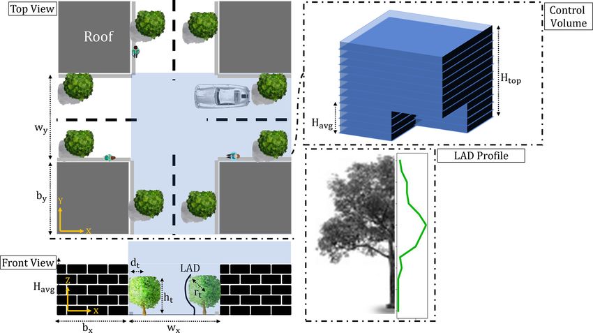
962                                                M. Moradi et al.: The Vertical City Weather Generator (VCWG v1.3.2)

atmospheric boundary layer (ABL; Britter and Hanna, 2003).        sult in the difficulty of parameterizations (Roth, 2000; Resler
Modeling enables a deeper understanding of interactions be-       et al., 2017). For example, the surfaces of urban obstacles ex-
tween urban areas and the atmosphere and can possibly offer       ert form and skin drag, consequently altering flow direction
solutions toward mitigating adverse effects of urban devel-       and producing eddies at different spatiotemporal scales. This
opment on the climate. A brief review of modeling efforts         can lead to the formation of shear layers at roof level with
is essential for more accurate model development toward an        variable oscillation frequencies (Tseng et al., 2006; Masson
understanding of urban area–atmosphere interactions.              et al., 2008; Zajic et al., 2011); all of such phenomena should
   Mesoscale models incorporating the urban climate were          be properly approximated in parameterizations.
initially aimed to resolve weather features with grid reso-           Heat exchanges between indoor and outdoor environ-
lutions of at best a few hundred meters horizontally and a        ments significantly influence the urban microclimate. Vari-
few meters vertically, without the functionality to resolve       ous studies have attempted to parametrize heat sources and
micro-scale three-dimensional flows or to account for at-         sinks caused by buildings such as heat fluxes due to in-
mospheric interactions with specific urban elements such          filtration, exfiltration, ventilation, walls, roofs, roads, win-
as roads, roofs, and walls (Bornstein, 1975). These mod-          dows, and building energy systems (e.g., condensers and ex-
els usually consider the effect of built-up areas by intro-       haust stacks) (Kikegawa et al., 2003; Salamanca et al., 2010;
ducing an urban aerodynamic roughness length (Grimmond            Yaghoobian and Kleissl, 2012). Therefore, a building en-
and Oke, 1999) or adding source or sink terms in the mo-          ergy model (BEM) is required to be properly integrated into
mentum (e.g., drag term) and potential temperature (e.g.,         an urban microclimate model to take account of the impact
anthropogenic heat term) equations (Dupont et al., 2004).         of building energy performance on the urban microclimate
Therefore, if higher grid resolutions less than 10 m (hori-       (Bueno et al., 2011, 2012b; Gros et al., 2014). This two-way
zontal and vertical) are desired (Moeng et al., 2007; Wang        interaction between the urban microclimate and indoor envi-
et al., 2009; Talbot et al., 2012), micro-scale climate mod-      ronment can significantly affect the urban heat island (UHI)
els should be deployed. Recently, multi-scale climate mod-        (K) and energy consumption of buildings (Salamanca et al.,
els have coupled mesoscale and micro-scale models (Chen           2014).
et al., 2011; Kochanski et al., 2015; Mauree et al., 2018).           Urban vegetation can substantially reduce the adverse ef-
Numerous studies have used computational fluid dynamics           fects of UHI (K), particularly during heat waves, resulting in
(CFD) to investigate the urban microclimate while taking          improved thermal comfort (Grimmond et al., 1996; Akbari
into account interactions between the atmosphere and urban        et al., 2001; Armson et al., 2012). Urban trees can potentially
elements with full three-dimensional flow analysis (Saneine-      provide shade and shelter, therefore changing the energy bal-
jad et al., 2012; Blocken, 2015; Nazarian and Kleissl, 2016;      ance of individual buildings in addition to the entire city (Ak-
Aliabadi et al., 2017; Nazarian et al., 2018). Despite accu-      bari et al., 2001). A study of the local-scale surface energy
rate predictions, CFD models are not computationally ef-          balance revealed that the amount of energy dissipated due to
ficient, particularly for weather forecasting at larger scales    the cooling effect of trees is not negligible and should be pa-
and for a long period of time, and they usually do not repre-     rameterized properly (Grimmond et al., 1996). In addition,
sent many processes in the real atmosphere such as clouds         the interaction between urban elements, most importantly
and precipitation. As an alternative, urban canopy models         trees and buildings, is evident in radiation trapping within
(UCMs) require understanding of the interactions between          the canyon and shading impact of trees (Krayenhoff et al.,
the atmosphere and urban elements to parameterize various         2014; Redon et al., 2017; Broadbent et al., 2019). Buildings
exchange processes of radiation, momentum, heat, and mois-        and trees obstruct the sky with implications for longwave
ture within and just above the canopy based on experimen-         and shortwave radiation fluxes both downward and upward
tal data, physical processes from theoretical considerations,     that may create unpredictable diurnal and seasonal changes
three-dimensional simulations, or simplified urban configu-       in UHI (K) (Kleerekoper et al., 2012; Yang and Li, 2015).
rations (Masson, 2000; Kusaka et al., 2001; Martilli et al.,      Also, it has been shown that not only trees but also the frac-
2002; Chin et al., 2005; Krayenhoff et al., 2014, 2015; Nazar-    tional vegetation coverage on urban surfaces can alter urban
ian and Kleissl, 2016; Aliabadi et al., 2019). These urban        temperatures with implications for UHI (K) (Armson et al.,
canopy models are more computationally efficient than CFD         2012). Trees, depending on their height and abundance rela-
models. They are designed to provide more details on heat         tive to buildings, could also exert drag and alter flow patterns
storage and radiation exchange, while they employ less de-        within the canopy; however, this effect is not as significant
tailed flow calculations.                                         as the drag induced by buildings (Krayenhoff et al., 2015).
   Urban microclimate models must account for a few unique        Such complex interactions must be accounted for in success-
features of the urban environment. Urban obstacles such as        ful urban microclimate models.
trees and buildings substantially contribute to changing flow
and turbulence patterns in cities (Kastner-Klein et al., 2004).
Difficulties arise when spatially inhomogeneous urban ar-
eas create highly three-dimensional wind patterns that re-

Geosci. Model Dev., 14, 961–984, 2021                                               https://doi.org/10.5194/gmd-14-961-2021
M. Moradi et al.: The Vertical City Weather Generator (VCWG v1.3.2)                                                           963

1.1   Research gaps                                               measured outside a city, without the need for mesoscale mod-
                                                                  eling, that are computationally efficient and operationally
Numerous studies have focused on high-fidelity urban mi-          simple for practical applications.
croclimate models with high spatiotemporal flow resolution,
capturing important features of the urban microclimate with       1.2   Objectives
acceptable accuracy (Gowardhan et al., 2011; Soulhac et al.,
2011; Blocken, 2015; Nazarian et al., 2018). Some exam-           In this study, we present a new urban microclimate model,
ple CFD models of this kind include Open-source Field Op-         called the Vertical City Weather Generator (VCWG), which
eration And Manipulation (OpenFOAM) (Aliabadi et al.,             attempts to overcome some of the limitations mentioned
2017, 2018), the Parallelized Large-Eddy Simulation Model         in the previous section. It resolves vertical profiles of cli-
(PALM) (Maronga et al., 2015; Resler et al., 2017), and           mate variables, such as potential temperature, wind, spe-
ENVI-met (Crank et al., 2018). Despite advances, however,         cific humidity, and turbulent kinetic energy in relation to
high-fidelity models capable of resolving three-dimensional       urban design parameters. VCWG also includes a building
flows at micro-scale are not computationally efficient and        energy model. It allows parametric investigation of design
are complex to implement for operational applications. As         options with urban climate control at multiple heights, par-
a remedy, lower-dimensional-flow urban microclimate mod-          ticularly if multistory building design options are consid-
els have been developed with many practical applications in       ered. This is a significant advantage over bulk flow (single-
city planning, architecture, and engineering consulting. For      layer) models such as UWG, which only consider one point
example, bulk flow (single-layer) models such as the Ur-          for flow dynamics inside a hypothetical canyon (Masson,
ban Weather Generator (UWG) calculate the flow dynam-             2000; Kusaka et al., 2001; Dupont et al., 2004; Krayen-
ics in one point, usually the center of a hypothetical ur-        hoff and Voogt, 2007; Lee and Park, 2008; Bueno et al.,
ban canyon, which is representative of all locations (Mills,      2012a, 2014). The advantages of VCWG are as follows. (1)
1997; Kusaka et al., 2001; Salamanca et al., 2010; Ryu            It does not need to be coupled to a mesoscale weather model
et al., 2011; Bueno et al., 2012a, 2014). Another bulk flow       because it functions stand-alone as a microclimate model. (2)
(single-layer) model is the Canyon Air Temperature (CAT)          Unlike many UCMs that are forced with climate variables
model, which utilizes standard data from a meteorological         above the urban roughness sublayer (e.g., TUF-3D), VCWG
station to estimate air temperature in a street canyon (Erell     is forced with rural climate variables measured at 2 m a.g.l.
and Williamson, 2006). The Town Energy Balance (TEB)              (temperature and humidity) and 10 m a.g.l. (wind) that are
model calculates energy balances for urban surfaces and is        widely accessible and available around the world, making
forced by meteorological data and incoming solar radiation        VCWG highly practical for urban design investigations in
at the urban site on top of the modeling domain (Masson           different climates. Further, unlike UWG, VCWG uses the
et al., 2002). The Temperatures of Urban Facets-3D (TUF-          Monin–Obukhov similarity theory in the rural area to con-
3D) model calculates urban surface temperatures with the          sider effects of thermal stability and aerodynamic, temper-
main focus on three-dimensional radiation exchange, but it        ature, and specific humidity roughness lengths to establish
adopts bulk flow (single-layer) modeling, and it is forced        vertical profiles of potential temperature and specific humid-
by meteorological data on top of its domain (Krayenhoff           ity. (3) VCWG provides urban climate information in one di-
and Voogt, 2007). More recently, TUF-3D was coupled to            mension, i.e., resolved vertically, which is advantageous over
an Indoor–Outdoor Building Energy Simulator (TUF-3D-              bulk flow (single-layer) models. (4) VCWG is coupled with
IOBES), but this model adopted a bulk flow (single-layer)         the building energy model using two-way interaction. (5) Un-
parameterization (Yaghoobian and Kleissl, 2012). The multi-       like UWG, VCWG considers the effect of trees in the urban
layer Building Effect Parametrization with Trees (BEP-Tree)       climate by modeling evapotranspiration (latent heat transfer),
model includes variable building heights, the vertical vari-      sensible heat transfer, radiation transfer, drag, and other pro-
ation of climate variables, and the effects of trees, but it is   cesses due to trees.
not linked to a building energy model (Martilli et al., 2002;        The paper is structured as follows. Section 2 describes the
Krayenhoff, 2014; Krayenhoff et al., 2020). More recently,        methodology, outlining the components of the VCWG model
the BEP model has been coupled to a building energy model         and their connections: the forcing EnergyPlusTM Weather
(BEP+BEM), but it is forced with meteorological variables         (EPW) dataset, the rural model (RM), the one-dimensional
from higher altitudes above a city using mesoscale models in-     vertical diffusion model, the building energy model, and the
stead of near-surface meteorological variables measured out-      radiation model. This section also describes the location and
side the city (rural areas). An overview of the literature re-    details of the BUBBLE field campaign used for model eval-
veals an apparent paucity of independent urban microclimate       uation. Section 3 provides the results and discussion. It starts
models that account for spatiotemporal variations of meteo-       with a detailed evaluation of VCWG by comparing simula-
rological parameters in the urban environment and consider        tion results with those of the BUBBLE field measurements.
the effects of trees, building energy, radiation, and the con-    Then, results from other explorations, including effects of
nection to the near-surface rural meteorological conditions       building dimensions, foliage density, building energy config-

https://doi.org/10.5194/gmd-14-961-2021                                                Geosci. Model Dev., 14, 961–984, 2021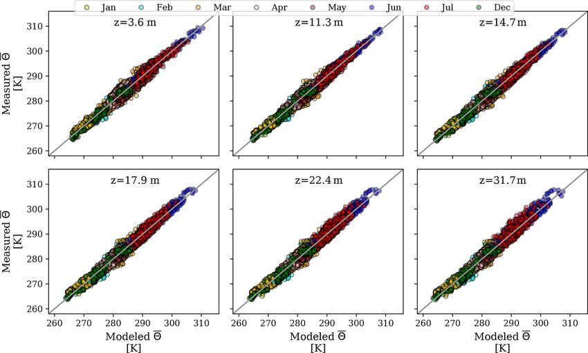
964 M. Moradi et al.: The Vertical City Weather Generator (VCWG v1.3.2)
uration, radiation configuration, seasonal variation, and dif- forced as boundary conditions to the one-dimensional verti-
ferent climate zones on the urban climate, are briefly pre- cal diffusion model in the urban area. The potential tempera-
sented with reference to the Supplement. Finally, Sect. 4 is ture and specific humidity are forced as fixed values on top of
devoted to conclusions and future work. Additional informa- the domain for the urban vertical diffusion model in the tem-
tion about the sub-models and equations used is provided in perature and specific humidity equations, respectively. The
Appendix A. horizontal pressure gradient is forced as a source term for the
urban vertical diffusion model in the momentum equation. It
must be acknowledged that the model does not consider hori-
2 Methodology zontal advection from the rural area. The model assumes that
the rural site is upwind of the urban site and the top of the
2.1 Vertical City Weather Generator (VCWG) domain is above the urban boundary layer. While forced by
the RM, the urban one-dimensional vertical diffusion model
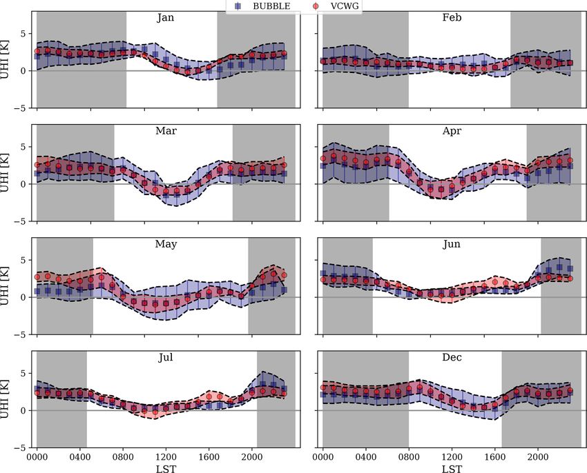
Figure 1 shows the VCWG model schematic. VCWG con- is also coupled with the building energy and radiation mod-
sists of four integrated sub-models: (1) a rural model (RM) els. The three models have feedback interaction. The urban
(Sect. 2.1.2) forces meteorological boundary conditions on one-dimensional vertical diffusion model calculates the flow
VCWG based on Monin–Obukhov similarity theory (Paul- quantities at the center of control volumes, which are gener-
son, 1970; Businger et al., 1971; Dyer, 1974) and a soil en- ated by splitting the urban computational domain into multi-
ergy balance model (Bueno et al., 2012a, 2014); (2) an ur- ple layers within and above the urban canyon (see Fig. 2).
ban one-dimensional vertical diffusion model (Sect. 2.1.3) is The urban domain extends to 3 times the building height
used for calculation of the vertical profiles of urban microcli- that conservatively falls closer to the top of the atmospheric
mate variables including potential temperature, wind speed, roughness sublayer in the urban area (Santiago and Martilli,
specific humidity, and turbulent kinetic energy considering 2010; Aliabadi et al., 2017) but within the inertial layer in the
the effect of trees, buildings, and the building energy system rural area, where Monin–Obukhov similarity theory can be
(e.g., condensers and exhaust stacks). This model was ini- applied (Basu and Lacser, 2017). In VCWG, buildings with
tially developed by Santiago and Martilli (2010) and Simón- uniformly distributed height, equal width, and equal spacing
Moral et al. (2017), while it was later ingested into another from one another represent the urban area. The feedback in-
model called the Building Effect Parametrization with Trees teraction coupling scheme among the building energy model,
(BEP-Tree) model, considering the effects of trees (Krayen- radiation model, and the urban one-dimensional vertical dif-
hoff, 2014; Krayenhoff et al., 2015, 2020). (3) A building fusion model is designed to update the boundary conditions,
energy model (BEM; Sect. 2.1.4) is used to determine the surface temperatures, and the source and sink terms in the
waste heat of buildings imposed on the urban environment. transport equations in successive time step iterations. More
This model is a component of the Urban Weather Generator details about the sub-models are provided in the subsequent
(UWG) model (Bueno et al., 2012a, 2014). (4) A radiation sections and Appendix A.
model with vegetation (Sect. 2.1.5) is used to compute the
longwave and shortwave heat exchanges between the urban
2.1.1 EnergyPlusTM weather data
canyon, trees, and the atmosphere and sky. A summary of this
model is provided by Meili et al. (2020) and the references
within. Building energy and solar radiation simulations are typically
The sub-models are integrated to predict vertical variations carried out with standardized weather files. EPW files in-
of urban microclimate variables including potential temper- clude recent weather data for 2100 locations and are saved
ature, wind speed, specific humidity, and turbulent kinetic in the standard EnergyPlusTM format developed by the US
energy as influenced by aerodynamic and thermal effects Department of Energy (https://energyplus.net/weather, last
of urban elements including longwave and shortwave radi- access: 10 February 2021). The data are available for most
ation exchanges, sensible heat fluxes released from urban el- North American cities, European cities, and other regions
ements, cooling effect of trees, and the induced drag by ur- around the world. The weather data are arranged by the
ban obstacles. The RM takes into account latitude, longitude, World Meteorological Organization (WMO) based on re-
dry bulb temperature, relative humidity, dew point tempera- gion and country. An EPW file contains typical hourly-based
ture and pressure at 2 m a.g.l., wind speed and direction at data for meteorological variables. The meteorological vari-
10 m a.g.l., downwelling direct shortwave radiation, down- ables are dry bulb temperature, dew point temperature, rela-
welling diffuse shortwave radiation, downwelling longwave tive humidity, incoming direct and diffusive shortwave radia-
radiation, and deep soil temperature from an EPW file. For tion fluxes from the sun and sky, respectively, incoming long-
every time step, and forced with the set of weather data, the wave radiation flux, wind direction, wind speed, sky condi-
RM then computes a potential temperature profile, a specific tion, precipitation (occasionally), deep soil temperature, and
humidity profile, friction velocity, and a horizontal pressure general information about field logistics and soil properties.
gradient as a function of friction velocity, all of which are Precipitation data are often missing in the EPW files.
Geosci. Model Dev., 14, 961–984, 2021 https://doi.org/10.5194/gmd-14-961-2021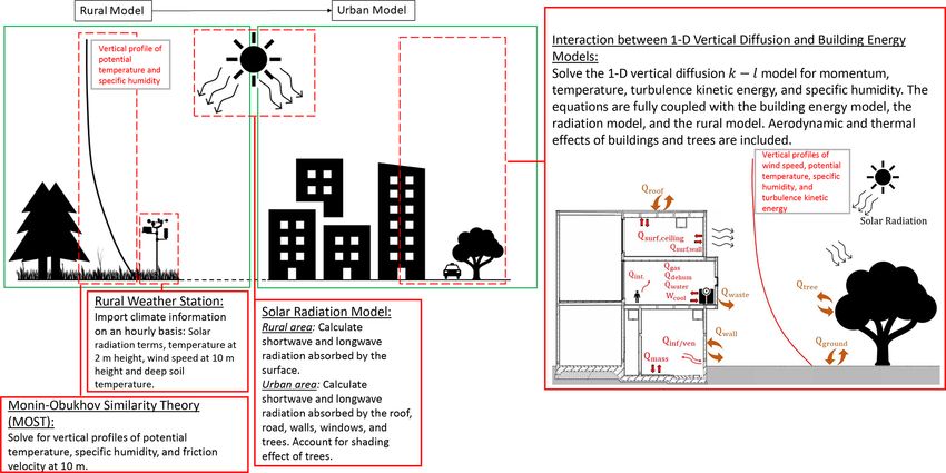
M. Moradi et al.: The Vertical City Weather Generator (VCWG v1.3.2)                                                               965

Figure 1. The schematic of the Vertical City Weather Generator (VCWG).

Figure 2. Simplified urban area used in VCWG and corresponding layers of control volumes within and above the canyon. The height of the
domain is 3 times the average building height. A leaf area density (LAD) (m2 m−3 ) profile is considered to represent trees.

2.1.2   Rural model                                                   humidity as functions of momentum flux, sensible heat flux,
                                                                      and latent heat flux measured near the surface, respectively.
                                                                      Using MOST the gradient of potential temperature is given
In the rural model, the Monin–Obukhov similarity theory
                                                                      by
(MOST) is used to solve for the vertical profiles of poten-
tial temperature, specific humidity, and friction velocity at         d2rur        Qsen,rur    z
10 m a.g.l. using meteorological measurements near the sur-                  =−             8H      ,                           (1)
                                                                        dz        ρCp κu∗ z     L
face. MOST is usually applied to the atmospheric surface
layer over flat and homogeneous land to describe the verti-           where 2rur (K) is mean potential temperature in the rural
cal profiles of wind speed, potential temperature, and specific       area, Qsen,rur (W m−2 ) is the net rural sensible heat flux, ρ

https://doi.org/10.5194/gmd-14-961-2021                                                    Geosci. Model Dev., 14, 961–984, 2021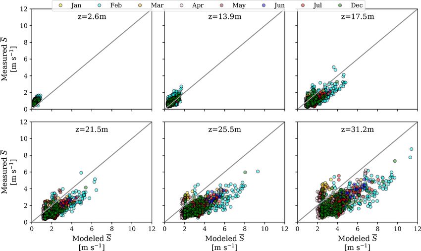
966 M. Moradi et al.: The Vertical City Weather Generator (VCWG v1.3.2)
(kg m−3 ) is air density near the rural surface, Cp (J kg−1 K−1 ) top of the domain). A typical formulation of z2,rur = 0.1z0rur
is air specific heat capacity, u∗ (m s−1 ) is friction veloc- (m) is often used (Brutsaert, 1982; Garratt, 1994; Järvi et al.,
ity, and κ = 0.4 (–) is the von Kármán constant. 8H (–) is 2011; Meili et al., 2020). This formulation is used in the
known as the universal dimensionless temperature gradient. present study.
This term is estimated for different thermal stability condi- Given the similarity of heat and mass transfer (sensible
tions based on experimental data by Businger et al. (1971) and latent heat fluxes), the same universal dimensionless
and Dyer (1974): temperature gradient can be used for the universal dimen-
sionless specific humidity gradient, i.e., 8Q = 8H (–) (Zeng
1 + 5 Lz , z
L > 0 (stable) and Dickinson, 1998). The net rural latent heat flux Qlat,rur
z
(W m−2 ) can either be directly measured or estimated using
z
8H = 1, L = 0 (neutral) (2)
L −1/2 the Bowen ratio βrur (–) and the net rural sensible heat flux
1 − 16z
, z
< 0 (unstable).
L L via Qlat,rur = Qsen,rur /βrur (W m−2 ). So the gradient of the
specific humidity can be given by the following expression,
In the dimensionless stability parameter z/L (–), z (m) is employing the latent heat of vaporization Lv (J kg−1 ), as
the height above ground and L (m) is the Obukhov length
given by dQrur Qlat,rur z
=− 8Q , (6)
−2rur,z=2m u3∗ dz ρLv κu∗ z L
L= Qsen,rur
. (3)
gκ which can also be integrated over height to give the vertical
ρCp
profile of specific humidity. This expression should be inte-
It has been observed that there is a monotonic reduction grated over height from the rural roughness length for spe-
in friction velocity with increasing stratification (Joffre et al., cific humidity zQ,rur (m) to z − drur (m), where z (m) is the
2001). So, friction velocity in Eq. (1) is estimated from mo- desired elevation above ground (here the top of the domain).
mentum flux generalization (Monin and Obukhov, 1954): It is often assumed that zQ,rur = z2,rur (m) (Brutsaert, 1982;
Järvi et al., 2011; Meili et al., 2020). This assumption is used
dS rur u∗ z
in the present study.
= 8M , (4)
dz κz L Meteorological information obtained from a weather sta-
tion, including direct and diffuse shortwave radiation, long-
where S rur (m s−1 ) is the mean horizontal wind speed in wave radiation, temperature at 2 m a.g.l., wind speed at
the rural area and 8M (–) is the universal dimensionless 10 m a.g.l., and deep soil temperature, is used to calculate the
wind shear estimated for different thermal stability condi- net rural sensible and latent heat fluxes at the surface via the
tions based on experimental data (Businger et al., 1971; surface energy balance:
Dyer, 1974).
QS,rur + QL,rur = Qsen,rur + Qlat,rur + Qgrd , (7)
1 + 5 Lz , z
L > 0 (stable)
z
where QS,rur and QL,rur (both in W m−2 ) are net shortwave
z
8M = 1, L = 0 (neutral) (5)
L
16z
−1/4
z
and longwave radiation fluxes at the surface (positive with
1− , < 0 (unstable)
L L energy flux into the surface), and Qsen,rur , Qlat,rur , and Qgrd
(all in W m−2 ) are net sensible, latent, and ground heat fluxes
Friction velocity can be determined by integrating Eq. (4) at the surface (positive with energy flux leaving the surface).
iteratively over height from the elevation of the rural aero- Appendix A details the calculation of each term.
dynamic roughness length z0rur (m) to z − drur (m), where The rural model also outputs a horizontal pressure gradient
z = 10 m is the reference height for wind measurement and based on the friction velocity calculation that is later used as a
drur (m) is the zero displacement height. The aerodynamic source term for the urban one-dimensional vertical diffusion
roughness length and zero displacement height have been momentum equation. The pressure gradient is parameterized
rigorously studied and parameterized in the literature as func- as ρu2∗ /Htop (kg m−2 s−2 ), where Htop (m) is the height of the
tions of obstacle height hrur (m) and the type of rural area top of the domain (Krayenhoff et al., 2015; Nazarian et al.,
(Raupach et al., 1991; Hanna and Britter, 2002). VCWG 2020), here 3 times the average building height.
permits this specification, but the approximate formulations After calculating potential temperature and specific hu-
used in this study are z0rur = 0.1hrur and drur = 0.5hrur . This midity at the top of the domain by the rural model, these
method provides a friction velocity that is corrected for ther- values can be applied as a fixed-value boundary condition
mal stability effects. at the top of the domain in the urban one-dimensional verti-
The potential temperature profiles are also obtained by in- cal diffusion model for the potential temperature and specific
tegration of Eq. (1) (Paulson, 1970) over height from the rural humidity transport equations.
roughness length for temperature z2,rur (m) to z − drur (m),
where z (m) is the desired elevation above ground (here the
Geosci. Model Dev., 14, 961–984, 2021 https://doi.org/10.5194/gmd-14-961-2021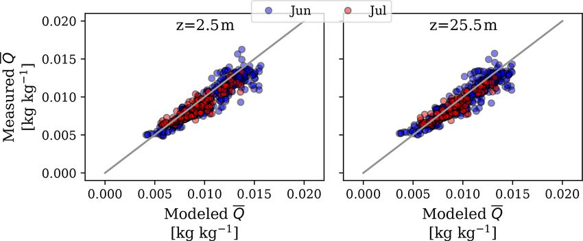
M. Moradi et al.: The Vertical City Weather Generator (VCWG v1.3.2) 967
2.1.3 Urban vertical diffusion model midity equations), where the diffusion coefficient is calcu-
lated using a k–` turbulence model,
Numerous studies have attempted to parameterize the inter-
action between urban elements and the atmosphere in terms Km = Ck `k k 1/2 , (10)
of dynamical and thermal effects, from very simple mod-
els based on MOST (Stull, 1988) to bulk flow (single-layer) where Ck (–) is a constant and `k (m) is a length scale op-
parameterizations (Krayenhoff and Voogt, 2007; Masson, timized using sensitivity analysis based on CFD (Nazarian
2000; Kusaka et al., 2001; Bueno et al., 2014) and multi- et al., 2020). Note that the plan area density λp (–) in this
layer models (Hamdi and Masson, 2008; Santiago and Mar- study is greater than the limit considered by Nazarian et al.
tilli, 2010; Krayenhoff et al., 2015, 2020) with different lev- (2020), so we assume that the parameterizations extrapolate
els of complexity. Multilayer models usually treat aerody- to this value of λp (–). More details on Ck (–) and `k (m) are
namic and thermal effects of urban elements as sink or source provided in Krayenhoff (2014) and Nazarian et al. (2020).
terms in potential temperature, momentum, specific humid- The turbulent kinetic energy k (m2 s−2 ) can be calculated us-
ity, and turbulent kinetic energy equations. Parameterization ing a prognostic equation (Krayenhoff et al., 2015):
of the exchange processes between urban elements and the !2 !2
atmosphere can be accomplished using either experimental ∂k ∂U ∂V
= Km + (11)
data or CFD simulations (Martilli et al., 2002; Dupont et al., ∂t ∂z ∂z
2004; Kondo et al., 2005; Kono et al., 2010; Lundquist et al., | {z }
2010; Santiago and Martilli, 2010; Krayenhoff et al., 2015; I
Aliabadi et al., 2019). CFD-based parameterizations pro-
∂ Km ∂k g Km ∂2
posed by Martilli and Santiago (2007), Santiago and Martilli + −
∂z σk ∂z 2 Pr ∂z
(2010), Krayenhoff et al. (2015), and Nazarian et al. (2020) | {z } | 0 {zt }
II III
use results from Reynolds-averaged Navier–Stokes (RANS)
or large-eddy simulations (LESs) including effects of trees ε ,
+ Swake − |{z}
| {z }
and buildings. These parameterizations consider the CFD re- IV V
sults at different elevations after being temporally and hori-
zontally averaged. where g (m s−2 ) is acceleration due to gravity and 20 (K)
For the one-dimensional vertical diffusion model, any is a reference potential temperature. The terms on the right-
variable such as cross- and along-canyon wind velocities hand side of Eq. (11) are shear production (I), turbulent trans-
(U and V , respectively; m s−1 ), potential temperature (2; port of kinetic energy parameterized based on K theory (II),
K), and specific humidity (Q; kg kg−1 ) is presented us- buoyant production and dissipation (III), wake production by
ing Reynolds averaging. The one-dimensional time-averaged urban obstacles and trees (IV), and dissipation (V). Parame-
momentum equations in the cross- and along-canyon compo- terizations of the last two terms are presented in more detail
nents can be shown as (Santiago and Martilli, 2010; Krayen- in Appendix A and by Krayenhoff (2014). σk (–) is the tur-
hoff, 2014; Krayenhoff et al., 2015, 2020; Simón-Moral bulent Prandtl number for turbulent kinetic energy, which is
et al., 2017; Nazarian et al., 2020) generally suggested to be σk = 1 (–) (Pope, 2000).
To calculate the vertical profile of potential temperature in
∂U ∂uw 1 ∂P the urban area, the energy transport equation can be derived
=− − − Dx , (8) as
∂t | ∂z
{z } |ρ {z
∂x |{z}
} III !
I II ∂2 ∂ Km ∂2
= (12)
∂t ∂z Prt ∂z
∂V ∂vw 1 ∂P
| {z }
=− − − Dy , (9) I
∂t | ∂z
{z } |ρ {z
∂y |{z} + S2R + S2G + S2W + S2V + S2A + S2waste ,
} III | {z }
I II II
where P (Pa) is time-averaged pressure. The terms on the where Prt (–) is the turbulent Prandtl number, the first term
right-hand side of Eqs. (8) and (9) are the vertical gradient of on the right-hand side is the turbulent transport of heat (I),
turbulent flux of momentum (I), acceleration due to the large- and the heat sink and source terms (II) correspond to sensi-
scale pressure gradient (II), and the sum of pressure, building ble heat exchanges with the roof (S2R ), ground (S2G ), walls
form, building skin, and vegetation drag terms (III). The pa- (S2W ), urban vegetation S2V , and radiative divergence S2A
rameterization of the latter term is detailed in Appendix A. K (all in K s−1 ). These terms are detailed in Appendix A and
theory is used to parameterize the vertical momentum fluxes, by Krayenhoff (2014). The contribution of waste heat emis-
i.e., uw = −Km ∂U /∂z and vw = −Km ∂V /∂z (the same ap- sions from the building heating ventilation and air condition-
proach will be used in potential temperature and specific hu- ing (HVAC) system S2waste (K s−1 ) is parameterized by
https://doi.org/10.5194/gmd-14-961-2021 Geosci. Model Dev., 14, 961–984, 2021968 M. Moradi et al.: The Vertical City Weather Generator (VCWG v1.3.2)
To complete the urban one-dimensional vertical diffusion
model, the transport equation for specific humidity is
1
S2waste = Fst QHVAC , (13) !
ρCp 1z ∂Q ∂ Km ∂Q
= + SQV , (16)
∂t ∂z Sct ∂z |{z}
where QHVAC (W m−2 ) is total sensible waste heat released | {z } II
into the urban atmosphere per building footprint area, Fst (– I
) is the fraction of waste heat released at street level, while where Q (kg kg−1 ) is time-averaged specific humidity. The
the remainder fraction (1 − Fst ) (–) is released at roof level, turbulent transport of specific humidity (I) is parameterized
and 1z (m) is grid discretization in the vertical direction. based on K theory, Sct (–) is the turbulent Schmidt number,
Depending on the type of building, waste heat emissions can and the source term SQV (Kg Kg−1 s−1 ) (II) is caused by la-
be partially released at street level and the rest at roof level, tent heat from vegetation as detailed in Appendix A and by
which can be adjusted by changing Fst (–) from 0 to 1. For Krayenhoff (2014).
the BUBBLE campaign, it is assumed that all waste heat was
released at roof level, which is more typical in most energy- 2.1.4 Building energy model
retrofitted mid-rise apartments (Christen and Vogt, 2004; Ro-
tach et al., 2005). The term QHVAC (W m−2 ) is calculated by In this study, the balance equation for convection, conduc-
the building energy model as tion, and radiation heat fluxes is applied to all building el-
ements (walls, roof, floor, windows, ceiling, and internal
QHVAC = Qsurf + Qven + Qinf + Qint (14) mass) to calculate the indoor air temperature. Then, a sen-
| {z } sible heat balance equation, between convective heat fluxes
Qcool
released from indoor surfaces and internal heat gains as well
+ Wcool + Qdehum + Qgas + Qwater , as sensible heat fluxes from the HVAC system and infiltra-
tion (or exfiltration), is solved to obtain the time evolution of
indoor temperature as
QHVAC = (Qsurf + Qven + Qinf + Qint )/ηheat (15) dTin
| {z } V
−ρCp = ±Qsurf ± Qven ± Qinf ± Qint , (17)
Qheat dt
− Qheat + Qdehum + Qgas + Qwater , where V − (m3 m−2 ) is indoor volume per building footprint
area, Tin (K) is indoor air temperature, and the heat fluxes
under cooling and heating modes, respectively. In this nota- on the right-hand side are specified in Eqs. (14) and (15).
tion all symbols represent positive quantities unless a neg- More details on parameterization of the terms in Eq. (17) can
ative quantity is emphasized by the negative sign in front be found in Appendix A and Bueno et al. (2012b). In this
of the symbol in the equation. Under cooling mode QHVAC notation all symbols represent positive quantities; however,
(W m−2 ) is calculated by adding the cooling demand (Qcool ; in the equation either positive or negative signs should be
W m−2 ), consisting of surface cooling demand, ventilation used to emphasize if a term contributes to indoor tempera-
demand, infiltration (or exfiltration) demand, internal en- ture increase or decrease, depending on the operation mode
ergy demand (lighting, equipment, and occupants), energy (cooling versus heating) and environmental conditions (in-
consumption of the cooling system (Wcool = Qcool /COP; door, outdoor, and surface temperatures).
W m−2 ; accounting for the coefficient of performance, COP, A similar balance equation can be derived for latent heat to
–), dehumidification demand (Qdehum ; W m−2 ), energy con- determine the time evolution of the indoor air specific humid-
sumption by gas combustion (e.g., cooking) (Qgas ; W m−2 ), ity and the dehumidification load Qdehum (W m−2 ), which is
and energy consumption for water heating (Qwater ; W m−2 ). parameterized in Bueno et al. (2012b). Note that energy con-
Under heating mode, QHVAC (W m−2 ) is calculated by sumption by gas combustion (e.g., cooking) Qgas and water
adding the heating demand (Qheat ; W m−2 ), consisting of heating Qwater (both in W m−2 ) does not influence indoor air
surface heating demand, ventilation demand, infiltration (or temperature or specific humidity, but such energy consump-
exfiltration) demand, and internal energy demand (lighting, tion sources appear in the waste heat equations: Eqs. (14)
equipment, and occupants) (divided by thermal efficiency of and (15). These terms are determined from schedules (Bueno
the heating system, ηheat ; –), then subtracting the heating et al., 2012b).
demand and adding the dehumidification demand (Qdehum ; The building energy model is a single-zone model with
W m−2 ), energy consumption by gas combustion (e.g., cook- respect to both the indoor and outdoor (urban canopy) envi-
ing) (Qgas ; W m−2 ) and energy consumption for water heat- ronments. That is, only a single temperature is assumed for
ing (Qwater ; W m−2 ). indoor air, and only a single potential temperature is assumed
for outdoor air by integrating the potential temperature pro-
file over height from the street to roof levels. Further, all wall
temperatures are assumed to be uniform with height.
Geosci. Model Dev., 14, 961–984, 2021 https://doi.org/10.5194/gmd-14-961-2021M. Moradi et al.: The Vertical City Weather Generator (VCWG v1.3.2) 969
2.1.5 Radiation model with vegetation et al., 2013). If trees are present, the view factors are cal-
culated with a simplified two-dimensional Monte Carlo ray-
In VCWG, there are two types of vegetation: ground veg- tracing algorithm (Wang, 2014; Frank et al., 2016). More de-
etation cover and trees. The ground vegetation cover frac- tails about the radiation model are provided in Appendix A
tion is specified by δs (–). Tree vegetation is specified by and by Meili et al. (2020).
four parameters: tree height ht (m), tree crown radius rt (m),
tree distance from canyon walls dt (m), and leaf area index 2.2 Experimental field campaigns
(LAI) (m2 m−2 ), which is the vertical integral of the leaf area
density (LAD) (m2 m−3 ) profile. VCWG considers two trees To evaluate the model, VCWG’s predictions are compared to
spaced from the walls of the canyon with distance dt (m). observations from the Basel UrBan Boundary Layer Exper-
Trees cannot be higher than the building height. Both types iment (BUBBLE) (Christen and Vogt, 2004; Rotach et al.,
of vegetation are specified with the same albedo αV (–) and 2005), which was conducted for 8 months from December
emissivity εV (–). The VCWG user can change these input 2001 to July 2002. The urban microclimate field measure-
parameters for different vegetation structures. The radiation ments were conducted in Basel, Switzerland, in a typical
model in VCWG is adapted from the model developed by quasi two-dimensional urban canyon (47.55◦ N and 7.58◦ E).
Meili et al. (2020). The net all-wave radiation flux is the sum An EPW file is used to force the VCWG simulations with
of the net shortwave and longwave radiation fluxes: rural measurements. The rural measurements correspond to
a site 7 km southeast of the city (47.53◦ N and 7.67◦ E). The
Rn = S ↓ − S ↑ + L↓ − L↑ , (18) average building height for the urban area is Havg = 14.6 m,
and the plan area density is λp = 0.54 (–). The urban canyon
where S ↓ , S ↑ , L↓ , and L↑ (all in W m−2 ) represent the in- axis is oriented in the northeast–southwest direction with a
coming shortwave, outgoing shortwave, incoming longwave, canyon axis angle of θcan = 65◦ . The x and y directions are
and outgoing longwave radiation fluxes. The incoming short- set to be cross- and along-canyon, respectively. The frontal
wave radiation fluxes (direct and diffuse) and the longwave area density is λf = 0.37 (–). In BUBBLE, potential tem-
radiation flux from the sky are forced by the EPW file. The perature was measured at z = 3.6, 11.3, 14.7, 17.9, 22.4,
absorbed (net) shortwave radiation on surface i is given by and 31.7 m a.g.l.; wind speed was measured at z = 2.5, 13.9,
17.5, 21.5, 25.5, and 31.2 m a.g.l.; and relative humidity was
↓ ↓direct ↓diffuse
Sn,i = (1 − αi ) Si = (1 − αi ) Si + Si , (19) measured at z = 2.5 and 25.5 m a.g.l. The dataset provides
the measurements averaged every 10 min. The model predic-
↓direct ↓diffuse tions of air temperature, wind speed, and specific humidity
where αi is the albedo of the surface, and Si and Si
(W m−2 ) are the direct and diffuse incoming shortwave ra- are compared to the observations on an hourly basis.
diation fluxes to surface i. Here, i can be S, G, V, W, or
T for sky, ground, ground vegetation, walls, and trees. The
3 Results and discussion
amount of direct shortwave radiation received by each ur-
ban surface is calculated considering shade effects accord- In this section, first the VCWG model results are evaluated
ing to well-established methodologies for the case with no against microclimate field measurements. Next, the model
trees (Masson, 2000; Kusaka et al., 2001; Wang et al., 2018) performance is explored through various parametric simula-
and with trees (Ryu et al., 2016). Sky view factors are used tions. A uniform Cartesian grid with 2 m vertical resolution
to determine the amount of diffuse shortwave radiation that is used. The flow is assumed to be pressure-driven with the
reaches a surface from the sky. Infinite reflections of diffuse pressure gradient of ρu2∗ /Htop (kgm−2 s−2 ), which is decom-
shortwave radiation are calculated within the urban canyon posed into the x and y directions based on the wind angle
with the use of view factors for each pair of urban surfaces and canyon orientation. This pressure gradient is forced as
(Wang, 2010, 2014). The absorbed (net) longwave radiation source terms on momentum Eqs. (8) and (9). The bound-
for each surface is calculated by ary conditions for potential temperature and specific humid-
↓
ity equations (Eqs. 12 and 16) are determined from the rural
Ln,i = εi Li − σ Ti4 , (20) model (see Fig. 1). Thus, the VCWG is aimed to calculate
momentum, temperature, specific humidity, and turbulent ki-
where εi (–) is the emissivity of the surface, (1 − εi ) (–) is netic energy exchanges for the center of each cell in the verti-
↓
the reflectivity of the surface, Li (W m−2 ) is the incoming cal direction based on the boundary conditions obtained from
longwave radiation flux, σ = 5.67 × 10⁻⁸ Wm−2 K−4 is the the rural model, the building energy model, and the radiation
Stefan–Boltzmann constant, and Ti (K) is the surface tem- model.
perature. Infinite reflections of longwave radiation within the
urban canyon are considered with the use of reciprocal view
factors. These view factors are analytically derived for the
case with no trees (Masson, 2000; Lee and Park, 2008; Wang
https://doi.org/10.5194/gmd-14-961-2021 Geosci. Model Dev., 14, 961–984, 2021970 M. Moradi et al.: The Vertical City Weather Generator (VCWG v1.3.2)
3.1 Detailed model–observation comparison RMSE, and R 2 of −0.1,K, 0.72,K, and 0.95 respectively,
near the ground. This comparison reveals that the bias and
3.1.1 Model input variables RMSE are improved (reduced) compared to the predecessor
UWG model.
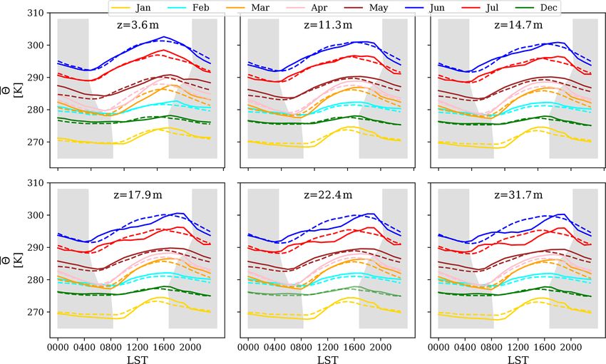
The results of the VCWG are compared to the measured data Figure 4 shows the diurnal variation of the observed versus
from the BUBBLE campaign. The input parameters repre- simulated values of potential temperature averaged for every
senting the urban area are listed in Table 1. The input pa- hour of the day for the available months. The diurnal pat-
rameters are inferred from variables, datasets, and simulation terns in temperature reveal that the model has similar skill in
codes in the literature that pertain to the BUBBLE campaign predicting the potential temperature during all hours at lower
and associated models as well as general assumptions found elevations (z = 3.6 to 14.7 m). This performance is compa-
in the literature (Raupach et al., 1991; Garratt, 1994; Hanna rable to other models that show a well-captured diurnal vari-
and Britter, 2002; Christen and Vogt, 2004; Järvi et al., ation of potential temperature at low altitudes (Bueno et al.,
2011; Bueno et al., 2012a; Faroux et al., 2013; Ryu et al., 2012a; Krayenhoff et al., 2020; Meili et al., 2020; Mussetti
2016; Yang et al., 2017; Meili et al., 2020; Mussetti et al., et al., 2020). However, the diurnal pattern in temperature can
2020). In this table, note that the choices of average build- deviate between the model and observations at higher eleva-
ing height Havg = 14.6 (m), street width w = 18.2 (m), and tions (z = 17.9 to 31.7 m), especially during midday hours.
the building width to street width ratio b/w = 1.1 (–) provide This can be attributed to more complex flow patterns in the
λp = b/(w + b) = 0.52 (–) and λf = Havg /(w + b) = 0.38 (– above-roof-level space due to heat advection, horizontal het-
), which are remarkably close to morphometric variables re- erogeneity of the urban site, and the above-roof-level shear
ported by Christen and Vogt (2004). The simulations are con- layer.
ducted for 8 months from December 2001 to July 2002. Usu-
ally the first 24 h of each month are treated as the model spin- 3.1.3 Wind speed
up period. For analysis of each month, the simulation time is
approximately 1 min; however, it can vary slightly depending Figure 5 and Table 3 show scatter plots of the observed ver-
on the grid spacing and time step. sus simulated values of wind speed and the statistical met-
rics used for the comparison. Considering all altitudes and
3.1.2 Potential temperature months, the average bias, RMSE, and R 2 are 0.67 m s−1 ,
1.06 m s−1 , and 0.41, respectively. Although the compari-
To compare VCWG results with measured meteorological son reveals a reasonable bias and RMSE, the R 2 is lower
variables from the BUBBLE campaign, the bias, root mean than values reported for comparisons of potential tempera-
square error (RMSE), and coefficient of determination R 2 are ture and specific humidity. This can be explained by the fact
computed for pairs of model versus observed values every that the urban morphology is highly heterogeneous, the mea-
hour for available altitudes and months. This analysis is per- surement of wind is location-specific, and the wind speed and
formed for wind speed, potential temperature, and specific direction can change considerably within each hour. Hetero-
humidity. Figure 3 and Table 2 show scatter plots of the ob- geneous urban morphology results in great spatial variabil-
served versus simulated values of potential temperature and ity of the components of wind velocity vector as a function
the statistical metrics used for the comparison. Over all alti- of wind direction and wind speed (Klein and Clark, 2007;
tudes and months, on average, the bias, RMSE, and R 2 for Klein and Galvez, 2015; Afshari and Ramirez, 2021). On the
potential temperature are 0.25 K, 1.41 K, and 0.82, respec- other hand, forced by hourly rural measurements, VCWG as-
tively. These statistics are comparable to what has been re- sumes a regular urban morphology and predicts the volume-
ported in the literature for similar models that were compared averaged horizontal wind velocity components. So it is ex-
against observations. For instance, Lauwaet et al. (2016) re- pected to obtain lower R 2 values. Other models also often
ported a bias, RMSE, and R 2 of 0.76 K, 1.32 K, and 0.88, report lower R 2 values for wind speed compared to poten-
respectively, near the ground by comparing model and obser- tial temperature and specific humidity (Mussetti et al., 2020).
vation values in summer. Meili et al. (2020) reported a bias, Overall, our bias, RMSE, and R 2 values are in agreement
RMSE, and R 2 of −0.1 K„ 2.2 K„ and 0.98 respectively, near with values reported in the literature. For instance, Lemonsu
the ground by comparing model and observation values in a et al. (2012) reported a range in bias of −0.16 to 0.56 m s−1 .
full year. Mussetti et al. (2020) reported a bias, RMSE, and They also reported a range in RMSE of 0.40 to 0.69 m s−1 .
R 2 of 0.40 K, 1.53 K, and 0.95, respectively, near the ground Mussetti et al. (2020) reported a bias, RMSE, and R 2 of
by comparing model and observation values in summer. Ryu 0.61 m s−1 , 1.31 m s−1 , and 0.70 , respectively.
et al. (2016) reported a bias and RMSE of 0.67 and 0.99 K,
respectively, near the ground by comparing model and ob- 3.1.4 Specific humidity
servation values in summer. Bueno et al. (2012a) reported
an average bias and RMSE of 0.6 and 0.9 K near the ground Figure 6 and Table 4 show scatter plots of the observed ver-
for June 2002. For the same month, VCWG predicts a bias, sus simulated values of specific humidity and the statisti-
Geosci. Model Dev., 14, 961–984, 2021 https://doi.org/10.5194/gmd-14-961-2021M. Moradi et al.: The Vertical City Weather Generator (VCWG v1.3.2) 971
Table 1. List of input parameters used in the VCWG for model evaluation; input variables are extracted from assumptions, datasets, and
simulation codes available from Raupach et al. (1991), Garratt (1994), Hanna and Britter (2002), Christen and Vogt (2004), Järvi et al.
(2011), Bueno et al. (2012a), Faroux et al. (2013), Ryu et al. (2016), Yang et al. (2017), Meili et al. (2020), and Mussetti et al. (2020).
Parameter Source Symbol Value
Latitude (◦ N) Christen and Vogt (2004) lat 47.55
Longitude (◦ E) Christen and Vogt (2004) long 7.58
Average building height (m) Christen and Vogt (2004) Havg 14.6
Width of canyon (m) Christen and Vogt (2004) wx = wy = w 18.2
Building width to canyon width ratio (–) Christen and Vogt (2004) bx /wx = by /wy = b/w 1.1
Leaf area index (m2 m−2 ) Faroux et al. (2013), Yang et al. (2017), LAI 0–1
Mussetti et al. (2020)
Tree height (m) Ryu et al. (2016) ht 8
Tree crown radius (m) Ryu et al. (2016) rt 2.5
Tree distance from wall (m) Ryu et al. (2016) dt 3
Ground vegetation cover fraction Ryu et al. (2016) δs 0
Building type Christen and Vogt (2004), Bueno et al. – Mid-rise apartment
(2012a)
Urban albedos (roof, ground, wall, vegeta- Bueno et al. (2012a), Ryu et al. (2016) αR , αG , αW , αV 0.15, 0.15, 0.15, 0.2
tion)
Urban emissivities (roof, ground, wall, veg- Bueno et al. (2012a), Ryu et al. (2016) εR , εG , εW , εV 0.95, 0.95, 0.95, 0.95
etation)
Rural overall albedo Bueno et al. (2012a) αrur 0.2
Rural overall emissivity Bueno et al. (2012a) εrur 0.95
Rural aerodynamic roughness length (m) Raupach et al. (1991), Bueno et al. z0rur = 0.1hrur 0.2
(2012a)
Rural roughness length for temperature (m) Garratt (1994), Meili et al. (2020) z2,rur = 0.1z0rur 0.02
Rural roughness length for specific humid- Järvi et al. (2011), Meili et al. (2020) zQ,rur = 0.1z0rur 0.02
ity (m)
Rural zero displacement height (m) Hanna and Britter (2002) drur = 0.5hrur 1
Rural Bowen ratio (–) Christen and Vogt (2004) βrur 0.9
Ground aerodynamic roughness length (m) Bueno et al. (2012a) z0 G 0.02
Roof aerodynamic roughness length (m) Bueno et al. (2012a) z0 R 0.02
Vertical resolution (m) – 1z 2
Time step (s) – 1t 60
Canyon axis orientation (◦ N) Christen and Vogt (2004) θcan 65
cal metrics used for the comparison. Note that specific hu- to the assumptions of the rural model to generate the vertical
midity data were only available in June–July 2002. Over profile of specific humidity. In this model the latent heat flux
all altitudes and the available months, on average, the bias, in the rural area is parameterized as a function of the sensible
RMSE, and R 2 for specific humidity are 0.00057 kg kg−1 , heat flux and a fixed Bowen ratio. However, the Bowen ra-
0.0010 kg kg−1 , and 0.85, respectively. These statistics are tio can vary diurnally (Kalanda et al., 1979). This can result
comparable to what has been reported in the literature for in a slight miscalculation of the latent heat flux and a forc-
similar models that were compared against observations. For ing boundary condition for specific humidity on top of the
instance, Mussetti et al. (2020) reported a bias, RMSE, and modeling domain.
R 2 of −0.00109 kg kg−1 , 0.00152 kg kg−1 , and 0.74, respec-
tively, above the urban canopy for comparisons of a model 3.1.5 Urban heat island (UHI)
and observations in summer. Lemonsu et al. (2012) reported
a range in bias of −0.00116 to −0.0005 kg kg−1 . They also To compare VCWG results with measured UHI (K) from
reported a range in RMSE of 0.00081 to 0.00172 kg kg−1 . the BUBBLE campaign, the bias, RMSE, and R 2 are com-
Figure 7 shows the diurnal variation of the observed ver- puted for pairs of hourly model versus observed values for
sus simulated values of specific humidity averaged for every the available months. UHI (K) for the observation is com-
hour of the day for June–July 2002. While the diurnal vari- puted by considering the difference between the temperature
ation is predicted by the model, some deviations are noted measurements inside the canyon at z = 3.6 m and tempera-
between the model and the observation. The model overpre- tures provided by the EPW dataset. For VCWG, UHI (K)
dicts the values at night, while it underpredicts the values is calculated by considering the difference between the tem-
during midday, especially at z = 25.5 m. This could be due perature prediction inside the canyon at z = 3 m and temper-
https://doi.org/10.5194/gmd-14-961-2021 Geosci. Model Dev., 14, 961–984, 2021972 M. Moradi et al.: The Vertical City Weather Generator (VCWG v1.3.2)
Figure 3. Scatter plots of observed (BUBBLE) versus simulated (VCWG) values of potential temperature for different altitudes and months;
each data point corresponds to a 1 h comparison between the model and observation.
Table 2. Bias (K), RMSE (K), and R 2 (–) for VCWG predictions of potential temperature against the BUBBLE observations for different
altitudes and months.
Altitude z (m) Statistic Dec Jan Feb Mar Apr May Jun Jul Average
Bias (K) 0.35 0.16 0.58 0.25 0.78 0.81 −0.1 −0.25 0.32
3.6 RMSE (K) 1.10 1.02 1.78 1.90 1.72 1.59 0.72 0.90 1.34
R2 0.97 0.70 0.80 0.72 0.62 0.89 0.95 0.88 0.82
Bias (K) 0.11 −0.19 0.60 0.23 0.50 0.87 −0.22 −0.23 0.21
11.3 RMSE (K) 1.07 1.17 1.7 1.84 1.59 1.34 0.79 0.96 1.31
R2 0.97 0.68 0.81 0.69 0.68 0.90 0.93 0.86 0.81
Bias (K) 0.20 −0.22 0.70 0.34 0.57 1.03 −0.12 −0.16 0.29
14.7 RMSE (K) 1.16 1.25 1.78 1.84 1.57 1.33 0.97 1.11 1.38
R2 0.96 0.66 0.81 0.70 0.71 0.89 0.92 0.87 0.82
Bias (K) 0.26 −0.21 0.75 0.36 0.55 0.99 −0.35 −0.35 0.25
17.9 RMSE (K) 1.19 1.27 1.82 1.85 1.54 1.30 1.14 1.31 1.43
R2 0.96 0.68 0.81 0.69 0.73 0.90 0.93 0.86 0.82
Bias (K) 0.29 −0.22 0.77 0.38 0.56 0.99 −0.45 −0.42 0.24
22.4 RMSE (K) 1.20 1.30 1.85 1.88 1.50 1.30 1.29 1.49 1.48
R2 0.96 0.68 0.81 0.68 0.74 0.90 0.93 0.86 0.82
Bias (K) 0.28 −0.28 0.78 0.37 0.58 0.95 −0.64 −0.57 0.18
31.7 RMSE (K) 1.17 1.35 1.87 1.90 1.52 1.31 1.43 1.69 1.53
R2 0.96 0.67 0.81 0.65 0.68 0.89 0.93 0.84 0.81
Bias (K) 0.25 −0.16 0.70 0.32 0.59 0.94 −0.31 −0.33 0.25
Average RMSE (K) 1.15 1.23 1.8 1.87 1.57 1.36 1.06 1.24 1.41
R2 0.96 0.68 0.81 0.69 0.69 0.90 0.93 0.86 0.82
Geosci. Model Dev., 14, 961–984, 2021 https://doi.org/10.5194/gmd-14-961-2021You can also read