Carbon Monitoring System Flux Net Biosphere Exchange 2020 (CMS-Flux NBE 2020) - ESSD
←
→
Page content transcription
If your browser does not render page correctly, please read the page content below
Earth Syst. Sci. Data, 13, 299–330, 2021
https://doi.org/10.5194/essd-13-299-2021
© Author(s) 2021. This work is distributed under
the Creative Commons Attribution 4.0 License.

                Carbon Monitoring System Flux Net Biosphere
                    Exchange 2020 (CMS-Flux NBE 2020)
               Junjie Liu1,2 , Latha Baskaran1 , Kevin Bowman1 , David Schimel1 , A. Anthony Bloom1 ,
           Nicholas C. Parazoo1 , Tomohiro Oda3,4 , Dustin Carroll5 , Dimitris Menemenlis1 , Joanna Joiner6 ,
             Roisin Commane7 , Bruce Daube8 , Lucianna V. Gatti9 , Kathryn McKain10,11 , John Miller10 ,
                               Britton B. Stephens12 , Colm Sweeney10 , and Steven Wofsy8
                    1 Jet  Propulsion Laboratory, California Institute of Technology, Pasadena, CA, USA
                                    2 California Institute of Technology, Pasadena, CA, USA
              3 Global Modeling and Assimilation Office, NASA Goddard Space Flight Center, Greenbelt, USA
                4 Goddard Earth Sciences Technology and Research, Universities Space Research Association,

                                                       Columbia, MD, USA
                   5 Moss Landing Marine Laboratories, San José State University, Moss Landing, CA, USA
       6 Laboratory for Atmospheric Chemistry and Dynamics, NASA Goddard Space Flight Center, Greenbelt, USA
                       7 Lamont-Doherty Earth Observatory of Columbia University, Palisades, NY, USA
                   8 Department of Earth and Planetary Sciences, Harvard University, Cambridge, MA, USA
               9 LaGEE, CCST, INPE – National Institute for Space Research, São José dos Campos, SP, Brazil
                               10 NOAA, Global Monitoring Laboratory, Boulder, CO 80305, USA
         11 Cooperative Institute for Research in Environmental Sciences, University of Colorado, Boulder, CO, USA
                            12 National Center for Atmospheric Research, Boulder, CO 80301, USA

                                 Correspondence: Junjie Liu (junjie.liu@jpl.nasa.gov)

                                    Received: 20 May 2020 – Discussion started: 7 July 2020
                    Revised: 21 December 2020 – Accepted: 23 December 2020 – Published: 10 February 2021

      Abstract. Here we present a global and regionally resolved terrestrial net biosphere exchange (NBE) dataset
      with corresponding uncertainties between 2010–2018: Carbon Monitoring System Flux Net Biosphere Exchange
      2020 (CMS-Flux NBE 2020). It is estimated using the NASA Carbon Monitoring System Flux (CMS-Flux) top-
      down flux inversion system that assimilates column CO2 observations from the Greenhouse Gases Observing
      Satellite (GOSAT) and NASA’s Observing Carbon Observatory 2 (OCO-2). The regional monthly fluxes are
      readily accessible as tabular files, and the gridded fluxes are available in NetCDF format. The fluxes and their
      uncertainties are evaluated by extensively comparing the posterior CO2 mole fractions with CO2 observations
      from aircraft and the NOAA marine boundary layer reference sites. We describe the characteristics of the dataset
      as the global total, regional climatological mean, and regional annual fluxes and seasonal cycles. We find that
      the global total fluxes of the dataset agree with atmospheric CO2 growth observed by the surface-observation
      network within uncertainty. Averaged between 2010 and 2018, the tropical regions range from close to neu-
      tral in tropical South America to a net source in Africa; these contrast with the extra-tropics, which are a net
      sink of 2.5 ± 0.3 Gt C/year. The regional satellite-constrained NBE estimates provide a unique perspective for
      understanding the terrestrial biosphere carbon dynamics and monitoring changes in regional contributions to
      the changes of atmospheric CO2 growth rate. The gridded and regional aggregated dataset can be accessed at
      https://doi.org/10.25966/4v02-c391 (Liu et al., 2020).

Published by Copernicus Publications.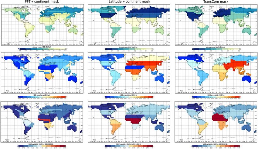
300                                                                                           J. Liu et al.: CMS-Flux NBE 2020

1   Introduction                                                    from OCO-2 is ∼ 1.0 ppm (Kulawik et al., 2019). A re-
                                                                    cent study by Byrne et al. (2020) shows less than a 0.5 ppm
New top-down inversion frameworks that harness satellite            difference between posterior XCO2 constrained by a recent
observations provide an important complement to global              dataset, ACOS-GOSAT b7 XCO2 retrievals, and those con-
aggregated fluxes (e.g., Global Carbon Budget (GCB),                strained by conventional surface CO2 observations. Cheval-
Friedlingstein et al., 2019) and inversions based on surface        lier et al. (2019) also showed that an OCO-2-based flux in-
CO2 observations (e.g., Chevallier et al., 2010), especially        version had similar performance to surface CO2 -based flux
over the tropics and the Southern Hemisphere (SH) where             inversions when comparing posterior CO2 mole fractions to
conventional surface CO2 observations are sparse. The net           aircraft CO2 in the free troposphere. Results from these stud-
biosphere exchange (NBE), which is the net carbon flux of all       ies show that systematic uncertainties in CO2 retrievals from
the land–atmosphere exchange processes except fossil fuel           satellites are comparable to, or smaller than, other uncer-
emissions, is far more variable and has far more uncertainty        tainty sources in atmospheric inversions (e.g., transport).
than ocean fluxes (Lovenduski and Bonan, 2017) or fossil               A newly developed biogeochemical model–data fusion
fuel emissions (Yin et al., 2019) and is thus the focus of this     system, CARDAMOM, made progress in producing NBE
dataset estimated from a top-down atmospheric CO2 inver-            uncertainties, along with mean values that are consistent with
sion of satellite column CO2 dry-air mole fraction (XCO2 ).         a variety of observations assimilated through a Markov chain
Here, we present the global and regional NBE as a series of         Monte Carlo (MCMC) method (Bloom et al., 2016, 2020).
maps, time series, and tables and disseminate it as a public        Transport model errors in general have also been reduced rel-
dataset for further analysis and comparison to other sources        ative to earlier transport model intercomparison efforts, such
of flux information. The gridded NBE dataset and its uncer-         as TransCom 3 (Gurney et al., 2004; Gaubert et al., 2019).
tainty, air–sea fluxes, and fossil fuel emissions are also avail-   Advancements in satellite retrieval, transport, and prior ter-
able so that users can calculate the carbon budget from a re-       restrial biosphere modeling have led to more mature inver-
gional to global scale. Finally, we provide a comprehensive         sions constrained by satellite XCO2 observations.
evaluation of both mean and uncertainty estimates against the          Two satellites, GOSAT and OCO-2, have now produced
CO2 observations from independent airborne datasets and the         more than 10 years of observations. Here we harness the
NOAA marine boundary layer (MBL) reference sites (Con-              NASA Carbon Monitoring System Flux (CMS-Flux) inver-
way et al., 1994).                                                  sion framework (Liu et al., 2014, 2017, 2018; Bowman et
    Global top-down atmospheric CO2 flux inversions have            al., 2017) to generate an NBE product – Carbon Moni-
been historically used to estimate regional terrestrial NBE.        toring System Flux Net Biosphere Exchange 2020 (CMS-
They make uses of the spatiotemporal variability of atmo-           Flux NBE 2020) – by assimilating both GOSAT and OCO-
spheric CO2 , which is dominated by NBE, to infer net car-          2 from 2010–2018. The dataset is the longest satellite-
bon exchange at the surface (Chevallier et al., 2005; Baker et      constrained NBE product so far. The CMS-Flux frame-
al., 2006a; Liu et al., 2014). The accuracy of the NBE from         work exploits globally available XCO2 to infer spatially re-
top-down flux inversions is determined by the density and           solved total surface–atmosphere exchange. In combination
accuracy of the CO2 observations, the accuracy of modeled           with constituent fluxes, e.g., gross primary production (GPP),
atmospheric transport, and knowledge of the prior uncertain-        NBE from CMS-Flux framework has been used to assess the
ties of the flux inventories.                                       impacts of El Niño on terrestrial biosphere fluxes (Bowman
    For CO2 flux inversions based on high precision in situ and     et al., 2017; Liu et al., 2017) and the role of droughts in
flask observations, the measurement error is low (< 0.2 ppm,        the North American carbon balance (Liu et al., 2018). These
parts per million) and not a significant source of error; how-      fluxes have furthermore been ingested into land–surface data
ever, these observations are limited spatially and are con-         assimilation systems to quantify heterotrophic respiration
centrated primarily over North America (NA) and Europe              (Konings et al., 2019), evaluate structural and parametric un-
(Crowell et al., 2019). Satellite XCO2 observations from CO2 -      certainty in carbon–climate models (Quetin et al., 2020), and
dedicated satellites, such as the Greenhouse Gases Observing        inform climate dynamics (Bloom et al., 2020). We present
Satellite (GOSAT) (launched in July 2009) and the Observ-           the regional NBE and its uncertainty based on three types of
ing Carbon Observatory 2 (OCO-2) (Crisp et al., 2017), have         regional masks: (1) latitude and continent, (2) distribution of
much broader spatial coverage (O’Dell et al., 2018), which          biome types (defined by plant functional types) and conti-
fills the observational gaps of conventional surface CO2 ob-        nent, and (3) TransCom regions (Gurney et al., 2004).
servations, but they have up to an order of magnitude higher           The outline of the paper is as follows: Sect. 2 describes
single-sounding uncertainty and potential systematic errors         methods, and Sects. 3 and 4 describe the dataset and the ma-
compared to the in situ and flask CO2 observations. Recent          jor NBE characteristics, respectively. We extensively evalu-
progress in instrument error characterization, spectroscopy,        ate the posterior fluxes and uncertainties by comparing the
and retrieval methods has significantly improved the accu-          posterior CO2 mole fractions against aircraft observations
racy and precision of the XCO2 retrievals (O’Dell et al., 2018;     and the NOAA MBL reference CO2 , as well as a gross pri-
Kiel et al., 2019). The single-sounding random error of XCO2        mary production (GPP) product (Sect. 5). In Sect. 6, we dis-

Earth Syst. Sci. Data, 13, 299–330, 2021                                             https://doi.org/10.5194/essd-13-299-2021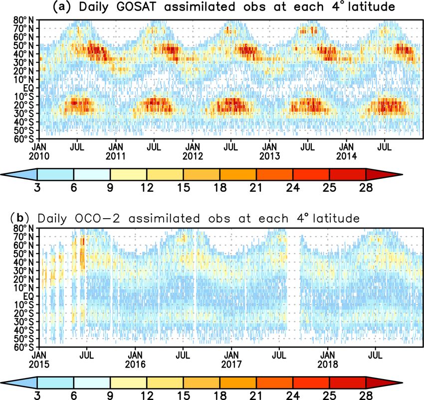
J. Liu et al.: CMS-Flux NBE 2020                                                                                                301

cuss the strength and weakness as well as potential usage of        time-resolved uncertainties in the NBE. The prior estimates
the data. A summary is provided in Sect. 7, and Sect. 8 de-         are already constrained with multiple data streams account-
scribes the dataset availability and future plan.                   ing for measurement uncertainties following a Bayesian
                                                                    approach similar to that used in the 4D-variational approach.
2     Methods                                                       We use the CARDAMOM setup as described by Bloom et
                                                                    al. (2016, 2020) resolved at monthly timescales; data
2.1    CMS-Flux inversion system                                    constraints include Global Ozone Monitoring Experiment 2
                                                                    (GOME-2) solar-induced fluorescence (Joiner et al., 2013),
The CMS-Flux framework is summarized in Fig. 1. The cen-            MODIS leaf area index (LAI), and biomass and soil carbon
ter of the system is the CMS-Flux inversion system, which           (details on the data assimilation are provided in Bloom et al.,
optimizes NBE and air–sea net carbon exchanges with a 4D-           2020). In addition, mean GPP and fire carbon emissions from
Var inversion system (Liu et al., 2014). In the current system,     2010–2017 are constrained by FLUXCOM RS + METEO
we assume no uncertainty in fossil fuel emissions, which is         version 1 GPP (Tramontana et al., 2016; Jung et al., 2017)
a widely adopted assumption in global flux inversion sys-           and GFEDv4.1s (Randerson et al., 2018), respectively,
tems (e.g., Crowell et al., 2019), since the uncertainty in fos-    both assimilated with an uncertainty of 20 %. We use
sil fuel emissions at regional scales is substantially less than    the Olsen and Randerson (2004) approach to downscale
the NBE uncertainties. The 4D-Var minimizes a cost function         monthly GPP and respiration fluxes to 3-hourly timescales,
that includes two terms:                                            based on ERA-Interim re-analysis of global radiation and
J (x) = (x − x b )T B−1 (x − x b )                                  surface temperature. Fire fluxes are downscaled using the
                                                                    GFEDv4.1 daily- and diurnal-scale factors on monthly emis-
       + (y − h(x))T R−1 (y − h(x)).                         (1)    sions (Giglio et al., 2013). Posterior CARDAMOM NBE
The first term measures the differences between the opti-           estimates are then summarized as NBE mean and standard
mized fluxes and the prior fluxes normalized by the prior           deviation values.
flux error covariance B. The second term measures the differ-          The NBE from CARDAMOM shows net carbon uptake
ences between observations (y) and the corresponding model          of 2.3 Gt C/year over the tropics and close to neutral in the
simulations (h(x)) normalized by the observation error co-          extra-tropics (Fig. B1). The year-to-year variability (i.e., in-
variance R. The term h (·) is the observation operator that cal-    terannual variability, IAV) estimated from CARDAMOM
culates observation-equivalent model-simulated XCO2 . The           is generally less than 0.1 g C/m2 /d outside of the tropics
4D-Var uses the adjoint (i.e., the backward integration of the      (Fig. B1). Because of the weak interannual variability esti-
transport model) (Henze et al., 2007) of the GEOS-Chem              mated by CARDAMOM, we use the same 2017 NBE prior
transport model to calculate the sensitivity of the observa-        for 2018.
tions to surface fluxes. The configurations of the inversion           CARDAMOM generates uncertainty along with the mean
system are summarized in Table 1. We run both the forward           state. The relative uncertainty over the tropics is generally
model and its adjoint at 4◦ × 5◦ spatial resolution and opti-       larger than 100 %, and the magnitude is between 50 % and
mize monthly NBE and air–sea carbon fluxes at each grid             100 % over the extra-tropics (Fig. B2). We assume no corre-
point from January 2010 to December 2018. Inputs for the            lation in the prior flux errors in either space or time. The tem-
system include prior carbon fluxes, meteorological drivers,         poral and spatial error correlation estimates can in principle
and the satellite XCO2 (Fig. 1). Sect. 2.2 (Table 2) describes      be computed by CARDAMOM. We anticipate incorporating
the prior flux and its uncertainties, and Sect. 2.3 (Table 3) de-   these error correlations in subsequent versions of this dataset.
scribes the observations and the corresponding uncertainties.
                                                                    2.3   Column CO2 observations from GOSAT and OCO-2
2.2    The prior CO2 fluxes and uncertainties
                                                                    We use the satellite-column CO2 retrievals from the Atmo-
The prior CO2 fluxes include NBE, air–sea carbon exchange,          spheric Carbon Observations from Space (ACOS) team for
and fossil fuel emissions (see Table 2). The data sources           both GOSAT (version 7.3) and OCO-2 (version 9) (Table 3).
for the prior fluxes are listed in Table 7 and provided in          The use of the same retrieval algorithm and validation strat-
the gridded fluxes. Methods to generate prior ocean carbon          egy adopted by the ACOS team to process both GOSAT
fluxes and fossil fuel emissions are documented in Brix et          and OCO-2 spectra maximizes the consistency between these
al. (2015), Caroll et al. (2020), and Oda et al. (2018). The fo-    two datasets. Both GOSAT and OCO-2 satellites carry high-
cus of this dataset is optimized terrestrial biosphere fluxes, so   resolution spectrometers optimized to return high-precision
we briefly describe the prior terrestrial biosphere fluxes and      measurements of reflected sunlight within CO2 and O2 ab-
their uncertainties.                                                sorption bands in the shortwave infrared (Crisp et al., 2012).
   We construct the NBE prior using the CAR-                        Both satellites fly in a sun-synchronous orbit. GOSAT has
DAMOM framework (Bloom et al., 2016). The CAR-                      a 13:00 ± 0.15 h local passing time and a 3 d ground track
DAMOM data assimilation system explicitly represents the            repeat cycle. The footprint of GOSAT is ∼ 10.5 km in diam-

https://doi.org/10.5194/essd-13-299-2021                                              Earth Syst. Sci. Data, 13, 299–330, 2021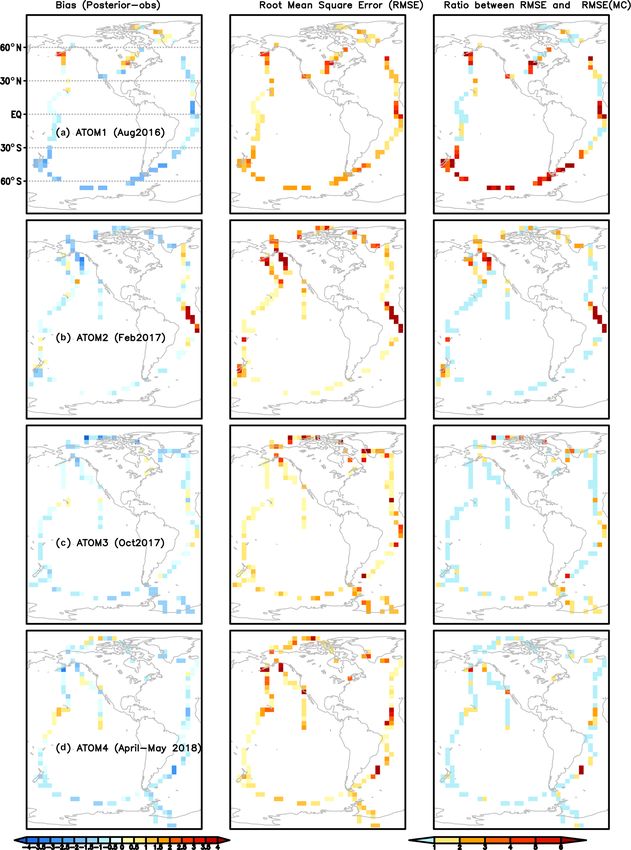
302                                                                                                  J. Liu et al.: CMS-Flux NBE 2020

Figure 1. Data flow diagram with the main processing steps to generate regional net biosphere exchange (NBE). TER: total ecosystem
respiration; GPP: gross primary production. The green box is the inversion system. The blue boxes are the inputs for the inversion system.
The red boxes are the data outputs from the system. The black box is the evaluation step, and the gray boxes are the future additions to the
product.

Table 1. Configurations of the CMS-Flux atmospheric inversion system.

                                      Model setup                    Configuration              Reference
            Inversion general setup   Spatial scale                  Global                     –
                                      Spatial resolution             4◦ latitude × 5◦ longi-
                                                                     tude
                                      Time resolution                monthly
                                      Minimizer of cost function     L-BFGS                     Byrd et al. (1994), Zhu et
                                                                                                al. (1997)
                                      Control vector                 Monthly net terrestrial
                                                                     biosphere fluxes and
                                                                     ocean fluxes
            Transport model           Model name                     GEOS-Chem and its          Suntharalingam et al. (2004),
                                                                     adjoint                    Nassar et al. (2010), Henze et
                                                                                                al. (2007)
                                      Meteorological forcing         GEOS-5 (2010–2014)         Rienecker et al. (2008)
                                                                     and GEOS-FP (2015–
                                                                     2019)

eter in sun nadir view (Crisp et al., 2012). The daily num-             super observations by aggregating the observations within
ber of soundings processed by the ACOS-GOSAT retrieval                  ∼ 100 km (along the same orbit) (Liu et al., 2017). The
algorithm is between a few hundred to ∼ 2000. Further qual-             super-obing strategy was first proposed in numerical weather
ity control and filtering reduce the ACOS-GOSAT XCO2 re-                prediction (NWP) to assimilate dense observations (Lorenc,
trievals to ∼ 100–300 daily (Fig. B5 in Liu et al., 2017).              1981) and is still broadly used in NWP (e.g., Liu and Ra-
We only assimilate ACOS-GOSAT land nadir observations                   bier, 2003). More detailed information about OCO-2 super
flagged as being good quality, which are the retrievals with            observations can be found in Liu et al. (2017). OCO-2 has
quality flag equal to zero.                                             four observing modes: land nadir, land glint, ocean glint, and
   OCO-2 has a 13:30 local passing time and 16 d ground                 target. Following Liu et al. (2017), we only use land nadir ob-
track repeat cycle. The nominal footprints of the OCO-2                 servations. The super observations have more uniform spatial
are 1.25 km wide and ∼ 2.4 km along the orbit. Because                  coverage and are more comparable to the spatial representa-
of its small footprints and sampling strategy, OCO-2 has                tion of ACOS-GOSAT observations and the transport model
many more XCO2 retrievals than ACOS-GOSAT. To reduce                    (see Fig. B5 in Liu et al., 2017).
the sampling error due to the resolution differences between               We directly use observational uncertainty provided with
the transport model and OCO-2 observations, we generate                 ACOS-GOSAT b7.3 to represent the observation error statis-

Earth Syst. Sci. Data, 13, 299–330, 2021                                                   https://doi.org/10.5194/essd-13-299-2021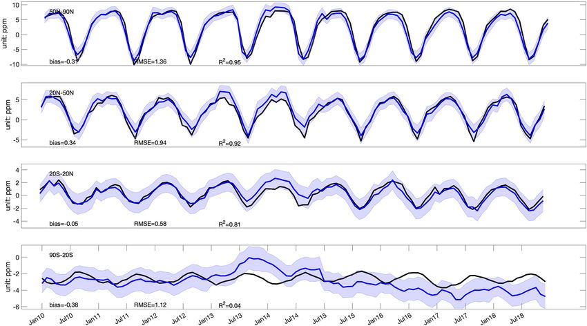
J. Liu et al.: CMS-Flux NBE 2020                                                                                                       303

Table 2. Description of the prior fluxes and assumed uncertainties in the inversion system.

           Prior fluxes         Terrestrial biosphere fluxes       Ocean fluxes                                Fossil fuel emissions
           Model name           CARDAMOM-v1                        ECCO-Darwin                                 ODIAC 2018
           Spatial resolution   4◦ × 5◦                            0.5◦                                        1◦ × 1◦
           Frequency            3-hourly                           3-hourly                                    Hourly
           Uncertainty          Estimated from CARDAMOM            100 % similar to Liu et al. (2017)          No uncertainty
           References           Bloom et al. (2016, 2020)          Brix et al. (2015), Carroll et al. (2020)   Oda et al. (2018)

Table 3. Description of observation and evaluation dataset. Data sources are listed in Table 7.

                                                      Dataset name and version             References
                   Satellite XCO2                     ACOS-GOSAT v7.3                      O’Dell et al. (2012)
                                                      OCO-2 v9                             O’Dell et al. (2018)
                   Aircraft CO2 observations          ObsPack OCO-2 MIP                    CarbonTracker team (2019)
                                                      HIPPO 3–5                            Wofsy et al. (2011)
                                                      ATom 1–4                             Wofsy et al. (2018)
                                                      INPE                                 Gatti et al. (2014)
                                                      ORCAS                                Stephens et al. (2017)
                                                      ACT-America                          Davis et al. (2018)
                   NOAA marine boundary layer         NOAA MBL reference                   Conway et al. (1994)
                   (MBL) reference
                   GPP                                FLUXSAT GPP                          Joiner et al. (2018)
                   Top-down NBE estimates con-        CarbonTracker Europe                 van der Laan-Luijkx            et
                   strained by surface CO2                                                 al. (2017)
                                                                                           Peters et al. (2010, 2007)
                                                      Jena               CarbonScope       Rödenbeck et al., 2003
                                                      s10oc_v2020
                                                      CAMS v18r1                           Chevallier et al. (2005)

tics, R, in Eq. (1). The uncertainty of the OCO-2 super obser-           from September 2014–June 2019 are used to optimize fluxes
vations is the sum of the variability of XCO2 used to gener-             between 2015 and 2018.
ate each individual super observation and the mean uncer-                   The observational coverage of ACOS-GOSAT and OCO-
tainty provided in the original OCO-2 retrievals. Kulawik                2 is spatiotemporally dependent, with more coverage during
et al. (2019) showed that both OCO-2 and ACOS-GOSAT                      summer than winter over the NH and more observations over
bias-corrected retrievals have a mean bias of −0.1 ppm when              midlatitudes than over the tropics (Fig. B3). The variability
compared with XCO2 from the Total Carbon Column Ob-                      (i.e., standard deviation) of the annual total number of ob-
serving Network (TCCON) (Wunch et al., 2011), indicating                 servations from 2010–2014 is within 4 % of the annual mean
consistency between ACOS-GOSAT and OCO-2 retrievals.                     number for ACOS-GOSAT. Except for a data gap in 2017
O’Dell et al. (2018) showed that the OCO-2 XCO2 land nadir               caused by a malfunction of the OCO-2 instrument, the vari-
retrievals have an RMSE of ∼ 1.1 ppm when compared to                    ability of the annual total number of observations between
TCCON retrievals; the differences between OCO-2 XCO2 re-                 2015 and 2018 is within 8 % of the annual mean number for
trievals and surface-CO2 -constrained model simulations are              OCO-2.
well within 1.0 ppm over most of the locations in the North-
ern Hemisphere (NH), where most of the surface CO2 obser-
vations are located.                                                     2.4    Uncertainty quantification
   The magnitude of observation errors used in R is gener-
ally above 1.0 ppm, larger than the sum of random error and              The posterior flux error covariance is the inverse Hessian,
biases in the observations. The ACOS-GOSAT b7.3 observa-                 which incorporates the transport, measurement, and back-
tions from July 2009–June 2015 are used to optimize fluxes               ground errors at the 4D-Var solution (Eq. 13 in Bowman et
between 2010 and 2014, and the OCO-2 XCO2 observations                   al., 2017). Posterior flux uncertainty projected to regions can
                                                                         be estimated analytically based on the methods described in

https://doi.org/10.5194/essd-13-299-2021                                                      Earth Syst. Sci. Data, 13, 299–330, 2021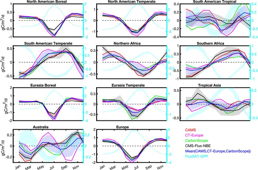
304                                                                                              J. Liu et al.: CMS-Flux NBE 2020

Fisher and Courtier (1995) and Meirink et al. (2008), using
either flux singular vectors or flux increments obtained dur-
ing the iterative optimization (e.g., Niwa and Fujii, 2020). In
this study, we rely on a Monte Carlo approach to quantify
posterior flux uncertainties following Chevallier et al. (2010)
and Liu et al. (2014), which is simpler and widely used.
In this approach, an ensemble of flux inversions is carried
out with an ensemble of priors and simulated observations
to sample the uncertainties of prior fluxes (i.e., B in Eq. 1)
and observations (R in Eq. 1), respectively. The magnitude
of posterior flux uncertainties is a function of assumed uncer-
tainties in prior fluxes and observations, as well as the density
of observations. Since the densities of GOSAT and OCO-
2 observations are stable (Sect. 2.3) within their respective
data record, we characterize the posterior flux uncertainties
for 2010 and 2015 only and assume the flux uncertainties for
2011–2014 are the same as 2010 and flux uncertainties for
2016–2018 are the same as 2015.

2.5     Evaluation of posterior fluxes

Direct NBE estimates from flux towers only provide a spa-
tial representation of roughly 1–3 km (Running et al., 1999),
which is not appropriate to evaluate regional NBE from top-
down flux inversions. Thus, we use two methods to indirectly
evaluate the posterior NBE and its uncertainties. One is to
compare annual NBE anomalies and seasonal cycle to a gross
primary production (GPP) product. The other is to compare
                                                                    Figure 2. The spatial and temporal distributions of aircraft observa-
posterior CO2 mole fractions to independent (i.e., not assimi-
                                                                    tions used in evaluation of posterior NBE. (a) The total number of
lated in the inversion) aircraft and the NOAA MBL reference         aircraft observations between 1–5 km between 2010–2018 at each
observations. The second method has been broadly used to            4◦ × 5◦ grid point. The rectangle boxes show the range of the nine
indirectly evaluate posterior fluxes from top-down flux in-         sub-regions. (b) The total number of monthly aircraft observations
versions (e.g., Stephens et al., 2007; Liu and Bowman, 2016;        at each longitude as a function of time.
Chevallier et al., 2019; Crowell et al., 2019). In addition
to these two methods, we also compare the NBE seasonal
cycles to three publicly available top-down NBE estimates           flux tower GPP observations and satellite-based geometry-
that are constrained by surface CO2 observations (Tables 3          adjusted reflectance from the Moderate Resolution Imag-
and 7).                                                             ing Spectroradiometer (MODIS) and solar-induced chloro-
                                                                    phyll fluorescence observations from GOME-2 (Joiner et al.,
2.5.1    Evaluation against the independent gross primary           2013). Joiner et al. (2018) show that the agreement between
         production (GPP) product                                   FLUXSAT GPP and GPP from flux towers is better than
                                                                    other available upscaled GPP products.
NBE is a small residual difference between two large terms:
total ecosystem respiration (TER) and GPP, plus fire. A pos-        2.5.2   Evaluation against aircraft and the NOAA marine
itive NBE anomaly (i.e., less uptake from the atmosphere)                   boundary layer (MBL) reference CO2 observations
has been shown to correspond to reduced GPP caused by
climate anomalies (e.g., Bastos et al., 2018), and the mag-         The aircraft observations used in this study include those
nitude of net uptake is proportional to GPP in most biomes          published in OCO-2 MIP ObsPack in August 2019 (Car-
observed by flux tower observations (e.g., Falk et al., 2008).      bonTracker team, 2019), which include regular vertical pro-
Since NBE is related not only to GPP, the comparison to             files from flask samples collected on light aircraft by NOAA
GPP only serves as a qualitative measure of the NBE qual-           (Sweeney et al., 2015) and other laboratories, regular (2- to 4-
ity. For example, we would expect the posterior NBE sea-            weekly) vertical profiles from the Instituto de Pesquisas Es-
sonality to be anti-correlated with GPP in the temperate and        paciais (INPE) over tropical South America (SA) (Gatti et al.,
high latitudes. In this study, we use FLUXSAT GPP (Joiner           2014), and vertical profiles from the Atmospheric Tomogra-
et al., 2018), which is an upscaled GPP product based on            phy (ATom, Wofsy et al., 2018), HIAPER Pole-to-Pole Ob-

Earth Syst. Sci. Data, 13, 299–330, 2021                                               https://doi.org/10.5194/essd-13-299-2021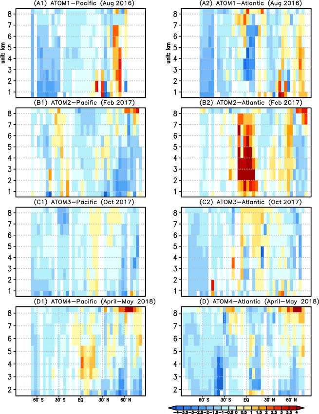
J. Liu et al.: CMS-Flux NBE 2020                                                                                                 305

servations (HIPPO, Wofsy et al., 2011), the O2 /N2 Ratio and          when the estimated posterior flux uncertainty reflects the true
CO2 airborne Southern Ocean Study (ORCAS) (Stephens et                posterior flux uncertainty, we show in the Appendix that
al., 2017), and Atmospheric Carbon and Transport – America
                                                                                         n
(ACT-America, Davis et al., 2018) aircraft campaigns (Ta-                             1X
                                                                      RMSE2 =               Ri,i + RMSE2MC ,                      (4)
ble 3). Figure 2 shows the aircraft observation coverage and                          n i=1
density between 2010 and 2018. Most of the aircraft obser-
vations are concentrated over NA. ATom had four (1–4) cam-            where Raircraft is the aircraft observation error variance,
paigns between August 2016 and May 2018, spanning four                which could be neglected on a regional scale.
seasons over the Pacific and Atlantic Ocean. HIPPO had five             We further calculate the ratio r between RMSE and
(HIPPO 1–5) campaigns over the Pacific, but only HIPPO 3–             RMSEMC :
5 occurred between 2010 and 2011. HIPPO 1–2 occurred in
                                                                            RMSE
2009. Based on the spatial distribution of aircraft observa-          r=          .                                               (5)
tions, we divide the comparison into nine regions: Alaska,                 RMSEMC
midlatitude NA, Europe, East Asia, South Asia, Africa, Aus-           A ratio close to one indicates that the posterior flux un-
tralia, Southern Ocean, and South America (Table 4 and                certainty reflects the true uncertainty in the posterior fluxes
Fig. 2).                                                              when the transport errors are small.
   We calculate several quantities to evaluate the posterior             The presence of transport errors will make the compar-
fluxes and their uncertainty with aircraft observations. One is       ison between RMSE and RMSEMC potentially difficult to
the monthly mean differences between posterior and aircraft           interpret. Even when RMSEMC represents the actual uncer-
CO2 mole fractions. The second is the monthly root mean               tainty in posterior fluxes, the RMSE could be larger than
square errors (RMSEs) over each of the nine sub-regions,              RMSEMC , since the differences between aircraft observa-
which is defined as                                                   tions and model-simulated posterior mole fraction RMSE
                                             !1                       could be due to errors in both transport and the posterior
               n                              2
            1X                                                        fluxes, while RMSEMC only reflects the impact of posterior
RMSE =           (y o         b
                           − yaircraft )2i        ,             (2)
            n i=1 aircraft                                            flux uncertainty on simulated aircraft observations. In this
                                                                      study, we assume the primary sources of RMSE come from
         o
where yaircraft                                    b
                 is the ith aircraft observation, yaircraft is the    errors in posterior fluxes.
corresponding posterior CO2 mole fraction sampled at the                 The RMSE and RMSEMC comparison only shows differ-
ith aircraft location, and n is the number of aircraft obser-         ences in CO2 space. We further calculate the sensitivity of the
vations over each region. The RMSE is computed over the               RMSE to the posterior flux using the GEOS-Chem adjoint.
n aircraft observations within one of the nine sub-regions.           We first define a cost function J as
The mean differences indicate the magnitude of the mean
posterior CO2 bias, while the RMSE includes both random               J = RMSE2 .                                                 (6)
and systematic errors in posterior CO2 . The bias and RMSE
                                                                      The sensitivity of the mean-square error to a flux, x, at loca-
could be due to errors in posterior fluxes, transport, and ini-
                                                                      tion i and month j is
tial CO2 concentrations. When errors in transport and initial
CO2 concentrations are smaller than the errors in the poste-                    ∂J
rior fluxes, the magnitude of biases and RMSE indicates the           wi,j =         × xi,j .                                     (7)
                                                                               ∂xi,j
accuracy of the posterior fluxes.
   To evaluate the magnitude of posterior flux uncertainty            This sensitivity is normalized by the flux magnitude. Equa-
estimates, we compare RMSE against the standard devia-                tion (7) can be interpreted as the sensitivity of the RMSE2 to
tion of ensemble simulated aircraft observations (Eq. 3) from         a fractional change in the fluxes. We can estimate the time-
the Monte Carlo method (RMSEMC ). The quantity RMSEMC                 integrated magnitude of the sensitivity over the entire assim-
can be written as                                                     ilation window by calculating
              "                                       #1                       M
          1 nens
               X        b(MC)           b(MC)
                                                        2                      P
                                                                                      wi,j
RMSEMC =            ((y       )iens − ȳaircraft )2         .   (3)
         nens iens=1 aircraft                                                  j =1
                                                                      Si =                     ,                                  (8)
                                                                             P P
                                                                             P M
                  b(MC)                                                                 wk,j
The variable (yaircraft )iens is the ith ensemble member of sim-             k=1 j =1
ulated aircraft observations from the Monte Carlo ensemble
               b(MC)
simulations, ȳaircraft is the mean, and nens is the total number     where P is the total number of grid points and M is the total
of ensemble members. For simplicity, in Eq. (3), we drop the          number of months from the time of the aircraft data to the be-
indices for the aircraft observations used in Eq. (2). In the         ginning of the inversion. The numerator of Eq. (8) quantifies
absence of errors in transport and initial CO2 concentrations,        the absolute total sensitivity of the RMSE2 to the fluxes at the

https://doi.org/10.5194/essd-13-299-2021                                                     Earth Syst. Sci. Data, 13, 299–330, 2021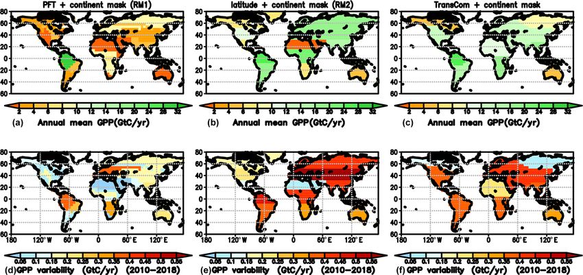
306                                                                                                J. Liu et al.: CMS-Flux NBE 2020

Table 4. Latitude and longitude ranges for seven sub-regions.

                  Region              Alaska          Midlatitude NA    Europe        East Asia          South Asia
                  Longitude range     180–125◦ W      125–65◦ W         5◦ W–45◦ E    110–160◦ E         65–110◦ E
                  Latitude range      58–89◦ N        22–58◦ N          30–66◦ N      22–50◦ N           10◦ S–32◦ N
                  Region              Africa          South America     Australia     Southern Ocean
                  Longitude range     5◦ W–55◦ E      95–50◦ W          120–160◦ E    110◦ W–40◦ E
                  Latitude range      2–18◦ N         20◦ S–2◦ N        45–10◦ S      80–30◦ S

ith grid. Normalized by the total absolute sensitivity across          compared to bottom-up extrapolated fluxes and Earth sys-
the globe, the quantity Si indicates the relative sensitivity of       tem models. Users can also aggregate the gridded fluxes and
RMSE2 to fluxes at the ith grid point. Note that Si is unit-           uncertainties based on their own defined regional masks. Ta-
less, and it only quantifies sensitivity, not the contribution of      ble 5 provides a complete list of all data products available in
fluxes at each grid to RMSE2 .                                         the dataset. In Sect. 4, we describe the major characteristics
   We use the NOAA MBL reference dataset (Table 7) to                  of the dataset.
evaluate the CO2 seasonal cycle over four latitude bands:
90–60◦ N, 60–20◦ N, 20◦ N–20◦ S, and 20–90◦ S. The MBL                 4     Characteristics of the dataset
reference is based on a subset of sites from the NOAA Coop-
erative Global Air Sampling Network. Only measurements                 4.1    Global fluxes
that are representative of a large of volume air over a broad
region are considered. In the comparison, we first remove              The annual atmospheric CO2 growth rate, which is the net
the global mean CO2 (https://www.esrl.noaa.gov/gmd/ccgg/               difference between fossil fuel emissions and total annual
trends/global.html, last access: 19 May 2020) from both the            sink over land and ocean, is well observed by the NOAA
NOAA MBL reference and the posterior CO2 .                             surface CO2 observing network (https://www.esrl.noaa.gov/
                                                                       gmd/ccgg/ggrn.php, last access: 12 March 2020). We com-
                                                                       pare the global total flux estimates constrained by GOSAT
2.6    Regional masks                                                  and OCO-2 with the NOAA CO2 growth rate from 2010–
                                                                       2018 and discuss the mean carbon sink over land and ocean.
We provide posterior NBE from 2010–2018 using three sets
                                                                       Over these 9 years, the satellite-constrained atmospheric
of regional masks (Fig. 3), in addition to the gridded prod-
                                                                       CO2 growth rate agrees with the NOAA observed CO2
uct. The regional mask in Fig. 3a is based on a combination
                                                                       growth rate within the uncertainty of the posterior fluxes
of seven plant function types condensed from MODIS IGBP
                                                                       (Fig. 4). The mean annual global surface CO2 fluxes (in
and the TransCom 3 regions (Gurney et al., 2004), which is
                                                                       Gt C/yr) are derived from the NOAA observed CO2 growth
referred to as Region Mask 1 (RM1) in the following de-
                                                                       rate (in ppm/yr) using a conversion factor of 2.124 Gt C/ppm
scription. There are 28 regions in Fig. 3a: six in NA, four in
                                                                       (Le Quéré et al., 2018). The estimated growth rate has the
SA, five in Eurasia (north of 40◦ N), three in tropical Asia,
                                                                       largest discrepancy with the NOAA observed growth rate in
three in Australia, and seven in Africa. The regional mask in
                                                                       2014, which may be due to a failure of one of the two solar
Fig. 3b is based on latitude and continents with 13 regions in
                                                                       paddles of GOSAT in May 2014 (Kuze et al., 2016). Over
total, which is referred to as Region Mask 2 (RM2) in later
                                                                       the 9 years, the estimated total accumulated carbon in the
description. Figure 3c is the TransCom regional mask with
                                                                       atmosphere is 41.5 ± 2.4 Gt C, which is slightly lower than
11 regions on land.
                                                                       the accumulated carbon based on the NOAA CO2 growth
                                                                       rate (45.2 ± 0.4 Gt C). On average, we estimate that the NBE
3     Dataset description                                              is 2.0 ± 0.7 Gt C, ∼ 20 ± 8 % of fossil fuel emissions, and
                                                                       the ocean sink is 3.0 ± 0.1 Gt C, ∼ 30 ± 1 % of fossil fuel
We present the fluxes as globally, latitudinally, and region-          emissions (Fig. 4). These numbers are within the ranges
ally aggregated time series. We show the 9-year average                of the corresponding GCB estimates from Freidlingstein et
fluxes aggregated into RM1, RM2, and TransCom regions                  al. (2019) (referred to as GCB-2019 hereafter). The mean
(Fig. 3). The aggregations are geographic (latitude and conti-         NBE and ocean sink from GCB-2019 are 2.0 ± 1.0 Gt C and
nent) and bio-climatic (biome by continent). For each region           2.5±0.5 Gt C, respectively, which are 21±10 % and 26±5 %
in the geographic and biome aggregations, we show 9-year               of fossil fuel emissions, respectively, between 2010–2018.
mean annual net fluxes and uncertainties and then the an-              The GCB does not report NBE directly, we calculate NBE
nual fluxes for each region as a set of time-series plots. The         from GCB-2019 as the residual differences between fossil
month-by-month fluxes and uncertainties are available in tab-          fuel emissions, ocean net carbon sink, and atmospheric CO2
ular format, so the actual aggregated fluxes may be readily            growth rate. It is also equivalent to (SLAND + BIM − ELUC )

Earth Syst. Sci. Data, 13, 299–330, 2021                                                https://doi.org/10.5194/essd-13-299-2021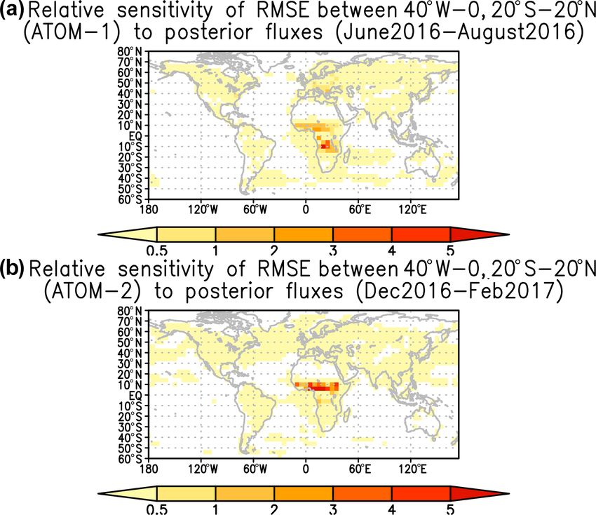
J. Liu et al.: CMS-Flux NBE 2020                                                                                                 307

Figure 3. Three types of regional masks used in calculating regional fluxes. (a) The mask is based on a combination of seven condensed
MODIS IGBP plant functional types, TransCom 3 regions (Gurney et al., 2004), and continents. (b) The mask is based on latitude and
continents. (c) The TransCom region mask.

https://doi.org/10.5194/essd-13-299-2021                                                Earth Syst. Sci. Data, 13, 299–330, 2021

308 J. Liu et al.: CMS-Flux NBE 2020
Figure 4. Global flux estimation and uncertainties from 2010–2018 (black: fossil fuel; green: posterior land fluxes; blue: ocean fluxes;
magenta: estimated CO2 growth rate; red: the NOAA CO2 growth rate).
reported by Freidlingstein et al. (2019), where SLAND is ter- e). We also find collocation of regions with large NBE and
restrial sink, BIM is a budget imbalance, and ELUC is land FLUXSAT GPP interannual variability (Fig. B4). The avail-
use change. Over these 9 years, we estimate that NBE ranges ability of flux estimates over the broadly used TransCom re-
from 3.6 Gt C (∼ 37 % of fossil fuel emissions) in 2011 (a La gions makes it easy to compare to previous studies. For ex-
Niña year) to only 0.5 Gt C (∼ 5 % of fossil fuel emissions) ample, we estimate that the annual net carbon uptake over
in 2015 (an El Niño year), consistent with 3.3 Gt C (35 % of North America is 0.7 ± 0.1 Gt C/yr with 0.2 Gt C variability
fossil fuel) in 2011 to 0.9 Gt C (7 % of fossil fuel) in 2015 between 2010 and 2018, which agrees with 0.7 ± 0.5 Gt C/yr
estimated from GCB-2019. We estimate that the ocean sinks estimates based on surface CO2 observations between 1996–
range from 3.5 Gt C in 2015 to 2.3 Gt C in 2012, which is 2007 (Peylin et al., 2013).
larger than the estimated ocean flux ranges of 2.7 in 2016 to
2.5 in 2012 reported by Freidlingstein et al. (2019).
4.3 Interannual variabilities and uncertainties
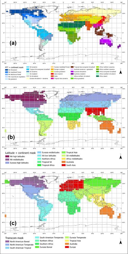
4.2 Mean regional fluxes and uncertainties Here we present hemispheric and regional NBE interannual
variabilities and corresponding uncertainties (Figs. 6 and 7,
Figure 5 shows the 9-year mean regional annual fluxes, un- and corresponding tabular data files). In Fig. 6, we further di-
certainty, and its variability between 2010–2018. Table 6 vide the globe into three large latitude bands: tropics (20◦ S–
shows an example of the dataset corresponding to Fig. 5a, 20◦ N), NH extra-tropics (20–85◦ N), and SH extra-tropics
d, and g. It shows that large net carbon uptake occurs over (60–20◦ S). The tropical NBE contributes 90 % to the global
Eurasia, NA, and the Southern Hemisphere (SH) midlati- NBE interannual variability (IAV). The IAV of NBE over the
tudes. The largest net carbon uptake is over the eastern US extra-tropics is only about one-third of that over the trop-
(−0.4 ± 0.1 Gt C (1σ uncertainty)) and high-latitude Eurasia ics. The dominant role of tropical NBE in the global IAV of
(−0.5 ± 0.1 Gt C) (Fig. 5a, b). We estimate a net land carbon NBE agrees with Fig. 4 in Sellers et al. (2018). The top-down
sink of 2.5 ± 0.3 Gt C/yr between 2010–2013 over the NH global annual NBE anomaly is within the 1.0 Gt C/yr uncer-
mid- to high latitudes, which agrees with 2.4 ± 0.6 Gt C esti- tainty of residual NBE (i.e., fossil fuel–atmospheric growth–
mates over the same time periods based on a two-box model ocean sink) calculated from GCB-2019 (Friedlinston et al.,
(Ciais et al., 2019). Net uptake in the tropics ranges from 2019) (Fig. 6).
close to neutral in tropical South America (0.1 ± 0.1 Gt C) to Figure 7 shows the annual NBE anomalies and uncertain-
a net source in northern Africa (0.6 ± 0.2 Gt C) (Fig. 5a, b). ties over a few selected regions based on RM1. Positive NBE
The tropics exhibit both large uncertainty and large variabil- indicates reduced net uptake relative to the 2010–2018 mean,
ity. The NBE interannual variabilities over northern Africa and vice versa. Also shown in Fig. 7 are GPP anomalies es-
and tropical SA are 0.5 and 0.3 Gt C, respectively, which timated from FLUXSAT. Positive GPP indicates increased
are larger than the 0.2 and 0.1 Gt C uncertainty (Fig. 5d, productivity, and vice versa. GPP drives NBE in years where
Earth Syst. Sci. Data, 13, 299–330, 2021 https://doi.org/10.5194/essd-13-299-2021J. Liu et al.: CMS-Flux NBE 2020 309 Figure 5. Mean annual regional NBE (a, b, c), uncertainty (d, e, f), and variability between 2010–2018 (g, h, i) with the three types of regional masks (Fig. 3). The first column uses a region mask based on plant functional types (PFTs) and continents (RM1). The second column uses a region mask based on latitude and continents (RM2), and the third column uses a TransCom mask. Figure 6. The NBE interannual variability over the globe (black), the tropics (20◦ S–20◦ N), SH midlatitudes (60–20◦ S), and NH midlat- itudes (20–90◦ N). For reference, the residual net land carbon sink from GCB-2019 (Friedlingstein et al., 2019) and its uncertainty is also shown (magenta). anomalies are inversely correlated (e.g., positive NBE and El Niño, corresponding to large reductions in productivity, negative GPP), and TER drives NBE in years where anoma- consistent with Liu et al. (2017). In 2017, the region sees lies of GPP and NBE have the same sign or are weakly increased net uptake and increased productivity, implying a correlated. Over tropical SA evergreen broadleaf forest, the recovery from the 2015–2016 El Niño event. The variabil- largest positive NBE anomalies occur during the 2015–2016 ity in GPP explains 80 % of NBE variability over this region https://doi.org/10.5194/essd-13-299-2021 Earth Syst. Sci. Data, 13, 299–330, 2021
310                                                                                             J. Liu et al.: CMS-Flux NBE 2020

Figure 7. The NBE interannual variability over six selected regions. Blue: annual NBE anomaly and its uncertainties. Green: annual GPP
anomaly based on FLUXSAT.

over the 9-year period. In Australian shrubland, our inver-          Laan-Luijkx et al., 2017), CAMS (Chevallier et al., 2005),
sion captures the increased net uptake in 2010 and 2011 due          and Jena CarbonScope (Rödenbeck et al., 2003). CMS-Flux
to increased precipitation (Poulter et al., 2014) and increased      NBE differs the most from surface-CO2 -based inversions
productivity. The variability in GPP explains 70 % of the in-        over the South American tropical, northern Africa, tropical
terannual variability in NBE. Over tropical South America            Asia, and NH boreal regions. The CMS-Flux NBE has a
savanna, the NBE interannual variability also shows strong           larger seasonal cycle amplitude over tropical Asia and north-
negative correlations with GPP, with GPP explaining 40 %             ern Africa, where the surface CO2 constraint is weak, while
of NBE interannual variability. Over the midlatitude regions         it has a smaller seasonal cycle amplitude over the boreal
where the IAV is small, the R 2 between GPP and NBE is               region; this may be due to the sparse satellite observations
also small (0.0–0.5) as expected. But the increased net uptake       over the high latitudes and weaker seasonal amplitude of the
generally corresponds to increased productivity. We also do          prior CARDAMOM fluxes. The comparison to FLUXSAT
not expect perfect negative correlation between NBE anoma-           GPP can only qualitatively evaluate the NBE seasonal cycle
lies and GPP anomalies, as discussed in Sect. 2.5. The com-          but cannot differentiate among different estimates. In gen-
parison between NBE and GPP provides insight into when               eral, the months that have larger productivity correspond to
and where net fluxes are likely dominated by productivity.           months with a net uptake of carbon from the atmosphere, es-
                                                                     pecially over the NH (Fig. 8). More research is still needed
4.4   Seasonal cycle                                                 to understand the seasonal cycles of NBE, including its phase
                                                                     (i.e., transition from source to sink) and amplitude (peak-to-
We provide the regional mean NBE seasonal cycle, its vari-           trough difference), as well as its relationships with GPP and
ability, and uncertainty based on the three regional masks           respiration.
(Table 5). Here we briefly describe the characteristics of the
NBE seasonal cycle over the 11 TransCom regions and its
comparison to three independent top-down inversion results
based on surface CO2 , which are CT-Europe (e.g., van der

Earth Syst. Sci. Data, 13, 299–330, 2021                                               https://doi.org/10.5194/essd-13-299-2021
J. Liu et al.: CMS-Flux NBE 2020 311
Table 5. List of the data products.
Product Spatial resolution Temporal resolution Data Sample data description
when applicable format in the text
Total fossil fuel, ocean, and Global Annual csv Fig. 4 (Sect. 4.1)
land fluxes
Climatology mean NBE, vari- PFT- and continent-based 28 re- n/a csv Fig. 5 (Sect. 4.2)
ability, and uncertainties gions
Geographic-based 13 regions csv
TransCom regions csv
Hemispheric NBE and uncer- NH (20–90◦ N), tropics (20◦ S– Annual csv Fig. 6 (Sect. 4.3)
tainties 20◦ N), and SH (60–20◦ S)
NBE variability and uncertain- PFT- and continent-based 28 re- Annual csv Fig. 7 (Sect. 4.3)
ties gions
Geographic-based 13 regions csv
TransCom regions csv
NBE seasonality and its uncer- PFT- and continent-based 28 re- Monthly csv Fig. 8 (Sect. 4.4)
tainties gions
Geographic-based 13 regions csv
TransCom regions csv
Monthly NBE and uncertainties PFT- and continent-based 28 re- Monthly csv n/a
gions
Geographic-based 13 regions csv
TransCom csv
Gridded posterior NBE, air–sea 4◦ (latitude) × 5◦ (longitude) Monthly NetCDF n/a
carbon exchanges, and uncer-
tainties
Gridded prior NBE and air–sea 4◦ (latitude) × 5◦ (longitude) Monthly and 3-hourly NetCDF n/a
carbon exchanges
Gridded fossil fuel emissions 4◦ (latitude) × 5◦ (longitude) Monthly mean and hourly NetCDF n/a
Region masks PFT- and continent-based 28 re- n/a csv Fig. 3 (Sect. 2.4)
gions
Geographic-based 13 regions
TransCom regions
n/a: not applicable.
5 Evaluation against independent aircraft CO2 umn of Fig. 9 show regional monthly mean detrended aircraft
observations CO2 observations (x axis) versus the simulated detrended
posterior CO2 (y axis). We used the NOAA global CO2 trend
5.1 Comparison to aircraft observations over nine to detrend both the observations and model-simulated mole
sub-regions fractions (ftp://aftp.cmdl.noaa.gov/products/trends/co2/co2_
trend_gl.txt, last access: 19 May 2020). Over the NH re-
In this section, we evaluate posterior CO2 against aircraft gions (Fig. 9a, b, c, d) and Africa (Fig. 9f), the R 2 is greater
observations over the nine sub-regions listed in Table 4 and than or equal to 0.9, which indicates that the posterior CO2
Fig. 2. We compare the posterior CO2 to aircraft CO2 mole captures the observed seasonality. The low R 2 (0.7) value
fractions above the planetary boundary layer and up to the in South Asia is caused by one outlier. Over the Southern
mid-troposphere (1–5 km) at the locations and time of air- Ocean, Australia, and SA, the R 2 is between 0.2 and 0.4, re-
craft observations, and then we calculate the monthly mean flecting weaker CO2 seasonality over these regions and pos-
error statistics between 1–5 km. The aircraft observations be- sible bias in ocean flux estimates (see discussions later).
tween 1–5 km are more sensitive to regional fluxes (Liu et al., The right panel of Fig. 9 shows the monthly mean dif-
2015; Liu and Bowman, 2016). Scatter plots in the left col- ferences between posterior CO2 and aircraft observations
https://doi.org/10.5194/essd-13-299-2021 Earth Syst. Sci. Data, 13, 299–330, 2021312 J. Liu et al.: CMS-Flux NBE 2020
Table 6. The 9-year mean regional annual fluxes, uncertainties, and variability. Regions are based on the mask shown in Fig. 5a (Figure5.csv).
Unit: Gt C/yr.
Region name (Figure4.csv) Mean NBE Uncertainty Variability
NA shrubland −0.14 0.02 0.05
NA needleleaf forest −0.22 0.04 0.06
NA deciduous forest −0.2 0.04 0.07
NA crop natural vegetation −0.41 0.06 0.18
NA grassland −0.04 0.03 0.03
NA savanna 0.03 0.02 0.03
Tropical South America (SA) evergreen broadleaf 0.04 0.1 0.28
SA savanna −0.09 0.06 0.18
SA cropland −0.07 0.03 0.07
SA shrubland −0.03 0.02 0.08
Eurasia shrubland savanna −0.44 0.07 0.14
Eurasia needleleaf forest −0.41 0.07 0.12
Europe cropland −0.46 0.09 0.16
Eurasia grassland 0.02 0.08 0.13
Asia cropland −0.37 0.13 0.08
India 0.14 0.09 0.14
Tropical Asia savanna −0.12 0.11 0.08
Tropical Asia evergreen broadleaf −0.09 0.09 0.12
Australian savanna grassland −0.11 0.02 0.09
Australian shrubland −0.07 0.01 0.05
Australian cropland −0.01 0.01 0.03
African northern shrubland 0.04 0.02 0.03
African grassland 0.03 0.01 0.01
African northern savanna 0.54 0.15 0.49
African southern savanna −0.27 0.18 0.33
African evergreen broadleaf 0.1 0.07 0.09
African southern shrubland 0.01 0.01 0.01
African desert 0.06 0.01 0.04
(black), RMSE (Eq. 2) (blue line), and RMSEMC (Eq. 3) (red and the actual posterior flux uncertainty over the regions that
line). The magnitude of the mean differences between the these aircraft observations are sensitive to. These aircraft ob-
posterior CO2 and aircraft observations is less than 0.5 ppm, servations are sensitive to NBE over a broad region as shown
except over the Southern Ocean, which has a −0.8 ppm bias. in Fig. B5. Note that Figs. B5 and B8–B10 are calculated
The mean differences between posterior CO2 and aircraft ob- using Eq. (8).
servations are primarily caused by errors in transport and
biases in assimilated satellite observations, while RMSEMC
is the internal flux error projected into mole fraction space. 5.2 Comparison to aircraft observations from ATom and
With the exception of the Southern Ocean, for all regions HIPPO aircraft campaigns
mean bias is significantly less than RMSEMC , which sug-
gests that transport and data bias in satellite observations Figures 10 and 11 show comparisons to aircraft CO2 from the
may be much smaller than the internal flux errors. Note that ATom 1–4 campaigns spanning four seasons and HIPPO 3–5
RMSEMC is smaller than RMSE over the first ∼ 6 months of over the Pacific Ocean between 1–5 km. The vertical curtain
simulation, which may indicate a dominant impact of errors comparisons are shown in Figs. B6 and B7. The mean dif-
in transport and initial CO2 concentration on posterior CO2 ferences between posterior CO2 and aircraft CO2 are quite
RMSE. uniform (within 0.5 ppm) throughout the column, except over
As demonstrated in Sect. 2.5, comparing RMSE and the Atlantic Ocean during ATom 1–2 and the Southern Ocean
RMSEMC is a test of the accuracy of posterior flux uncer- during ATom 1 (Figs. S6 and S7). Also shown in Figs. 10
tainty estimate. Over all the regions, the differences between and 11 are RMSEs of each aircraft campaign (middle col-
RMSE and RMSEMC are smaller than 0.3 ppm, which in- umn) and the ratio between RMSE and RMSEMC (right col-
dicates a comparable magnitude between empirical poste- umn). A ratio larger than one between RMSE and RMSEMC
rior flux uncertainty estimates from the Monte Carlo method indicates errors in either transport or underestimation of the
posterior flux uncertainty (Sect. 2.5).
Earth Syst. Sci. Data, 13, 299–330, 2021 https://doi.org/10.5194/essd-13-299-2021J. Liu et al.: CMS-Flux NBE 2020 313 Figure 8. The NBE climatological seasonality over TransCom regions. The seasonal cycle is calculated over 2010–2017 since CT-Europe only covers until 2017. Black: CMS-Flux NBE and its uncertainty; blue shaded: mean NBE seasonality based on surface CO2 inversion results from CAMS, CT-Europe, and Jena CarbonScope; red: CAMS; magenta: CT-Europe; green: Jena CarbonScope. The names of each region are shown on individual subplots. Over most of the flight tracks during ATom 1–4, the pos- fined in Eq. (7). The adjoint sensitivity analysis indicates that terior CO2 errors are between −0.5 and 0.5 ppm, the RMSE the large mismatch between aircraft observations and model is smaller than 0.5 ppm, and the ratio between RMSE and simulations during ATom 1 and -2 off the coast of Africa RMSEMC is smaller than or equal to 1. However, off the coast could be potentially driven by errors in posterior fluxes over of Africa during ATom 1 and 2 and over the Southern Ocean tropical Africa (Fig. B8). The large posterior CO2 errors and during ATom 1, the mean differences between posterior CO2 large ratio between RMSE and RMSEMC over the Southern and aircraft observations are larger than 0.5 ppm. During Ocean during ATom 1 are driven by flux errors in oceanic ATom 1 (29 July–23 August 2016), the mean differences be- fluxes around 30◦ S and over Australia (Fig. B9), which also tween posterior CO2 and aircraft CO2 show large negative contribute to the large errors in comparison to aircraft obser- biases, while during ATom 2 (26 January–21 February 2017) vations over the Southern Ocean shown in Fig. 9h. it has large positive biases off the coast of Africa. The ra- During the HIPPO aircraft campaigns, the absolute errors tio between RMSE and RMSEMC is significantly larger than in posterior CO2 across the Pacific are less than 0.5 ppm, one over these regions, which indicates an underestimation except over the Arctic Ocean and over Alaska in summer of posterior flux uncertainty or a large magnitude of trans- (Fig. 11), consistent with Fig. 10a. The large errors over the port errors during that time period. Arctic Ocean may be related to both transport errors and the We further run adjoint sensitivity analyses over the three accuracy of high-latitude fluxes. Byrne et al. (2020) provide a regions with ratios significantly larger than one to identify brief summary of the challenges in simulating CO2 over high the posterior fluxes that could contribute to the large dif- latitudes using a transport model with 4◦ × 5◦ resolution. In- ferences between posterior CO2 and aircraft observations creasing the resolution of the transport model may reduce during ATom 1–2. We run the adjoint model backward for transport errors over high latitudes. 3 months from the observation time and calculate Si as de- https://doi.org/10.5194/essd-13-299-2021 Earth Syst. Sci. Data, 13, 299–330, 2021
314                                                                                                 J. Liu et al.: CMS-Flux NBE 2020

Figure 9. Comparison between posterior CO2 mole fraction and aircraft observations. Left panel: detrended posterior CO2 (y axis) vs. de-
trended aircraft CO2 (x axis) over nine regions. The dashed line is the one-to-one line; right panel: the differences between posterior CO2
and aircraft CO2 as a function of time (black), RMSE (blue; unit: ppm), and RMSEMC (red).

   We run adjoint sensitivity analyses over the high-latitude           Over 90–20◦ S, the posterior CO2 has positive bias in 2013
regions where the differences between posterior CO2 and air-            and 2014 and negative bias and much weaker seasonality be-
craft observations are large (Fig. 11). The adjoint sensitivity         tween January 2015–December 2018 compared to observa-
analysis (Fig. B10) shows that the large errors over these re-          tions, which indicates possible biases in Southern Ocean flux
gions could be driven by errors in fluxes over Alaska as well           estimates (Fig. B11). The low bias over the Southern Ocean
as broad NH midlatitude regions.                                        is consistent with aircraft comparison during the OCO-2 pe-
                                                                        riod (Figs. 9–10, B9). The changes of performance after 2013
                                                                        over 90–20◦ S are most likely due to the prior ocean carbon
5.3   Comparison to MBL reference sites
                                                                        fluxes. Evaluation of ocean carbon fluxes is out of the scope
Since MBL reference sites sample air over broad regions, the            of this study. Note that since we only assimilate land nadir
comparison to detrended MBL observations indirectly eval-               XCO2 observations in this study due to known issues with the
uates the NBE over large regions. Figure 12 shows the com-              OCO-2 v9 ocean glint observations (O’Dell et all., 2018), the
parison over four latitude bands. The uncertainty of poste-             constraint of top-down inversion on air–sea CO2 exchanges
rior CO2 concentration is from the MC method. Except over               is weak (not shown). The ocean glint observations of OCO-2
90–20◦ S, the differences between observations and poste-               v10 observations have been improved compared to v9 (Os-
rior CO2 are within posterior CO2 uncertainty estimates. The            terman et al., 2020). We expect to have a better estimate of
posterior CO2 concentrations have the smallest bias and ran-            ocean carbon fluxes over the Southern Ocean when assimi-
dom errors over the tropical latitude band. The R 2 is above            lating both land and ocean XCO2 observations from GOSAT
0.9 over NH mid- to high latitudes, consistent with Fig. 9.             and OCO-2 in the future.

Earth Syst. Sci. Data, 13, 299–330, 2021                                                  https://doi.org/10.5194/essd-13-299-2021
You can also read