A new view of heat wave dynamics and predictability over the eastern Mediterranean
←
→
Page content transcription
If your browser does not render page correctly, please read the page content below
Earth Syst. Dynam., 12, 133–149, 2021
https://doi.org/10.5194/esd-12-133-2021
© Author(s) 2021. This work is distributed under
the Creative Commons Attribution 4.0 License.

            A new view of heat wave dynamics and predictability
                      over the eastern Mediterranean
           Assaf Hochman1 , Sebastian Scher2 , Julian Quinting1 , Joaquim G. Pinto1 , and Gabriele Messori2,3
         1 Department  of Tropospheric Research, Institute of Meteorology and Climate Research, Karlsruhe Institute
                                             of Technology, Karlsruhe, Germany
                            2 Department of Meteorology and Bolin Centre for Climate Research,

                                          Stockholm University, Stockholm, Sweden
                 3 Department of Earth Sciences and Centre of Natural Hazards and Disaster Science (CNDS),

                                            Uppsala University, Uppsala, Sweden
                                  Correspondence: Assaf Hochman (assaf.hochman@kit.edu)

                                       Received: 3 June 2020 – Discussion started: 8 July 2020
                        Revised: 1 December 2020 – Accepted: 17 December 2020 – Published: 4 February 2021

       Abstract. Skillful forecasts of extreme weather events have a major socioeconomic relevance. Here, we com-
       pare two complementary approaches to diagnose the predictability of extreme weather: recent developments
       in dynamical systems theory and numerical ensemble weather forecasts. The former allows us to define atmo-
       spheric configurations in terms of their persistence and local dimension, which provides information on how the
       atmosphere evolves to and from a given state of interest. These metrics may be used as proxies for the intrinsic
       predictability of the atmosphere, which only depends on the atmosphere’s properties. Ensemble weather forecasts
       provide information on the practical predictability of the atmosphere, which partly depends on the performance
       of the numerical model used. We focus on heat waves affecting the eastern Mediterranean. These are identified
       using the climatic stress index (CSI), which was explicitly developed for the summer weather conditions in this
       region and differentiates between heat waves (upper decile) and cool days (lower decile). Significant differences
       are found between the two groups from both the dynamical systems and the numerical weather prediction per-
       spectives. Specifically, heat waves show relatively stable flow characteristics (high intrinsic predictability) but
       comparatively low practical predictability (large model spread and error). For 500 hPa geopotential height fields,
       the intrinsic predictability of heat waves is lowest at the event’s onset and decay. We relate these results to the
       physical processes governing eastern Mediterranean summer heat waves: adiabatic descent of the air parcels
       over the region and the geographical origin of the air parcels over land prior to the onset of a heat wave. A
       detailed analysis of the mid-August 2010 record-breaking heat wave provides further insights into the range of
       different regional atmospheric configurations conducive to heat waves. We conclude that the dynamical systems
       approach can be a useful complement to conventional numerical forecasts for understanding the dynamics and
       predictability of eastern Mediterranean heat waves.

1   Introduction                                                    Williams, 2014; Caldeira et al., 2015). Moreover, heat waves
                                                                    are projected to increase in frequency, intensity and persis-
Heat waves are recognized as a major natural hazard (e.g.,          tence under global warming (e.g., Meehl and Tebaldi, 2004;
Easterling et al., 2000), causing detrimental socioeconomic         Stott et al., 2004; Fischer and Schär, 2010; Seneviratne et
impacts (e.g., “Feeling the heat”, 2018), including excess          al., 2012; Russo et al., 2014). The eastern Mediterranean has
mortality (e.g., Batisti and Naylor, 2009; Benett et al., 2014;     experienced several extreme heat waves in recent decades
Peterson et al., 2013; Ballester et al., 2019), agricultural loss   (e.g., Kuglitsch et al., 2010), and their frequency and inten-
(e.g., Deryng et al., 2014) and ecosystem impairment (e.g.,

Published by Copernicus Publications on behalf of the European Geosciences Union.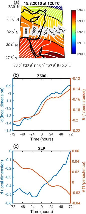
134                                                                    A. Hochman et al.: A new view of heat wave dynamics

sity are expected to increase in the coming decades (e.g.,         lute record for this station since 1942. The ability to predict
Giorgi, 2006; Seneviratne et al., 2012; Lelieveld et al., 2016;    and issue appropriate warnings for these types of events (and
Hochman et al., 2018a) upon a background of regional warm-         more generally weather events lying in the tails of the re-
ing and drying (e.g., Barchikovska et al., 2020).                  spective distributions) is of crucial importance to mitigate the
   The eastern Mediterranean climate is characterized by wet       impacts on human life, agriculture and ecosystems (IPCC,
conditions and mild air temperatures during the winter sea-        2012; Siebert and Evert, 2014; Williams, 2014).
son and dry and hot weather conditions during summer (e.g.,           A general framework that allows a quantitative under-
Kushnir et al., 2017). The summer season is characterized by       standing of processes leading to extreme temperatures dur-
very small inter-daily variability, which is attributable to the   ing heat waves is that based on Lagrangian backward trajec-
dominant and persistent influence of the Persian trough and        tories. In this framework, the temperature of an air parcel in-
subtropical high-pressure systems. The interaction between         creases by (i) adiabatic warming related to descent and (ii) di-
these systems leads to persistent northwesterly winds of con-      abatic heating including latent and sensible heat fluxes, short-
tinental origin blowing across the Aegean Sea. These winds         wave radiation and long-wave radiation (Holton, 2004). Re-
have been known as “Etesian winds” since ancient times             cent studies have revealed that extreme temperatures during
(Tyrlis and Lelieveld, 2013). Together with the Mediter-           heat waves are most often a combination of adiabatic warm-
ranean Sea breeze, moist air can be transported inland (Alpert     ing related to descent and diabatic heating near the surface
et al., 1990; Bitan and Saaroni, 1992) as far as the Dead Sea      (e.g., Black et al., 2004; Bieli et al., 2015; Santos et al., 2015;
(Kunin et al., 2019). In the upper levels of the Troposphere,      Quinting and Reeder, 2017; Zschenderlein et al., 2019). The
large-scale subsidence is dominant, thereby further hamper-        adiabatic warming is typically associated with upper-level
ing the development of clouds and precipitation (Rodwell           ridges, which promote subsidence. The strongest diabatically
and Hoskins, 1996; Ziv et al., 2004). In spite of this gen-        driven heating does not necessarily occur at the location of
erally low variability, heat waves are not infrequent during       the heat wave itself but rather in geographically remote re-
the summer (Harpaz et al., 2014). Still, episodes when the         gions (e.g., Quinting and Reeder, 2017; Quinting et al., 2018;
temperature drops to below normal values do occur, some of         Zschenderlein et al., 2019).
which are accompanied by summer rains (Saaroni and Ziv,               Focusing more directly on the prediction of the evolu-
2000).                                                             tion of specific atmospheric configurations, which may lead
   Saaroni et al. (2017) detected weaknesses in the ability of     to heat waves, one may consider a partly model-dependent
earlier synoptic classifications (Alpert et al., 2004a; Dayan      perspective (practical predictability) or a model-independent
et al., 2012) to describe local weather conditions during the      perspective (intrinsic predictability; Melhauser and Zhang,
eastern Mediterranean summer season. The authors proposed          2012). The practical predictability is heavily reliant on the
a “climatic stress index” (CSI), which is a combination of the     availability of initialization data (Lorenz, 1963) and on the
national heat stress index, used operationally by the Israeli      correct representation of relevant physical processes in the
Meteorological Service, and the height of the marine inver-        numerical model being used. However, it also reflects some
sion base height (see Sect. 2.2). The authors argued that this     characteristics of the atmospheric dynamics (e.g., Ferranti
novel index improves the classification of heat wave days rel-     et al., 2015; Matsueda and Palmer, 2018). A commonly
ative to earlier classifications and additionally links directly   used method for quantifying the practical predictability is
to the potential impacts.                                          the spread or skill of ensemble forecasts (e.g., Loken et al.,
   A notable heat wave in recent years was the 2010 so-            2019).
called “Russian heat wave”, which caused ∼ 55 000 excess              As opposed to the practical predictability, the intrinsic pre-
deaths in eastern Europe and western Russia (e.g., Barriope-       dictability only depends on the characteristics of the atmo-
dro et al., 2011; Katsafados et al., 2014). The 2010 North-        sphere itself. However, it is important to note that the atmo-
ern Hemisphere summer saw a strong and persistent block-           sphere is influenced and sometimes even controlled by in-
ing ridge at 500 hPa over the Middle East and eastern Europe       teractions with the land and oceans, albeit mostly at longer
(e.g., Grumm, 2011; Schneidereit et al., 2012; Quandt et al.,      timescales than those considered in this study (Entin et
2017), leading to unprecedented temperatures at numerous           al., 2000; Koster et al., 2010; Dirmeyer et al., 2018). Re-
locations (Barriopedro et al., 2011). The eastern Mediter-         cent developments in dynamical systems theory allow us to
ranean and Israel experienced a record-breaking (with re-          quantify the intrinsic predictability of instantaneous atmo-
spect to temperature) heat wave during mid-August of that          spheric states using two metrics: persistence (θ −1 ) and lo-
year (https://ims.gov.il/sites/default/files/aug10.pdf, last ac-   cal dimension (d). These reflect how the atmosphere evolves
cess: 2 November 2020), which interestingly coincided with         in the neighborhood of a state of interest (Faranda et al.,
what is considered the decay phase of the Russian heat wave        2017a). High (low) θ −1 (d) implies high intrinsic predictabil-
(Quandt et al., 2019). In fact, the Zefat Har-Knaan station        ity, whereas low (high) θ −1 (d) suggests low intrinsic pre-
(Table S1; Fig. S1) recorded a temperature of 40.6 ◦ C – the       dictability. The two forms of atmospheric predictability de-
highest temperature since 1939 – while the Jerusalem station       pend on different factors and, therefore, offer different infor-
(Table S1; Fig. S1) logged a remarkable 41 ◦ C – the abso-         mation. While there is some relation between the two (e.g.,

Earth Syst. Dynam., 12, 133–149, 2021                                                  https://doi.org/10.5194/esd-12-133-2021
A. Hochman et al.: A new view of heat wave dynamics                                                                         135

Scher and Messori, 2018), one should not expect them to al-       forecast and a 10-member ensemble on a 0.5◦ × 0.5◦ grid
ways match for individual cases (Hochman et al., 2020a).          spacing.
   In the present study, we perform a systematic dynami-             Finally, we make use of a homogenized station dataset
cal systems investigation of the temporal evolution of east-      over Israel to assess the forecasts. Instrumental meteorologi-
ern Mediterranean summer heat waves and evaluate whether          cal records may be influenced by non-meteorological events,
this may provide insights complementary to a more conven-         such as station relocation, defects in the instrumentation and
tional analysis of the numerical weather forecasts of such        environmental changes near the station. The detrimental ef-
events. Specifically, we hypothesize that the dynamical sys-      fects that these may have on the quality of the recorded data
tems analysis captures relevant features of these extremes,       can be reduced by homogeneity procedures (Aguilar et al.,
such as their persistence, which are not always reflected         2003). Our dataset includes five representative, homogenized
in the numerical weather forecast. The dynamical systems          stations in Israel with an uninterrupted record of maximum
framework has recently been leveraged for the study of cold       temperatures over 1979–2015 (Table S1, Fig. S1; Yosef et al.,
spell dynamics (Hochman et al., 2020a).                           2018).
   The paper is organized as follows: Sect. 2 provides a brief
description of the methodology, including the used datasets,      2.2   Heat wave definition according to the climatic stress
the CSI index, the dynamical systems and forecast skill met-            index (CSI)
rics as well as the method for backtracking air parcels. Sec-
tion 3 describes the dynamics of heat waves from both the         Saaroni et al. (2017) proposed a new index for classifying
dynamical system and the numerical weather prediction per-        the summer days over the eastern Mediterranean based on
spectives and further provides a detailed analysis of the mid-    the “environment to climate” approach (Yarnal, 1993; Yarnal
August 2010 heat wave over the eastern Mediterranean as a         et al., 2001). The CSI is comprised of the national heat stress
case study. Finally, Sect. 4 provides the main conclusions and    index, used operationally by the Israel Meteorological Ser-
discusses ideas for future research.                              vice, and the marine inversion base height, which is a major
                                                                  factor influencing the summer weather conditions over the
                                                                  eastern Mediterranean (Ziv et al., 2004). The index suits the
2     Data and methods                                            identification of heat waves as it does not merely consider the
                                                                  daily temperature but rather additional variables, e.g., humid-
2.1    Data                                                       ity and circulation, which directly relate to the impacts of a
The bulk of our analysis is based on the National Centers for     heat wave on factors such as human physiology (Epstein and
Environmental Prediction/National Center for Atmospheric          Moran, 2006). Saaroni et al. (2017) rigorously evaluated the
Research (NCEP/NCAR) Reanalysis project daily and 6-              CSI index with respect to observations and tested a variety
hourly reanalysis data for 1979–2015 (satellite era), on a        of different combinations of predictors, which ultimately re-
2.5◦ × 2.5◦ horizontal grid (Kalnay et al., 1996). Faranda        sulted in a simple multiple regression equation:
et al. (2017a) showed that the conclusions one may infer          CSI = 92.78 + 0.638T1000–850 − 0.1781p − 1.08pIraq .       (1)
from the dynamical systems analysis are generally insensi-
tive to the dataset’s horizontal spatial resolution, as long as   Here, T1000–850 is the average regional lower-level tempera-
the major structures characterizing the atmospheric field of      ture over the region from 31 to 34◦ N and 33 to 37◦ E. 1p
interest are resolved. On the contrary, the air parcel tracking   is the average sea level pressure over the region from 36 to
(Sect. 2.5) requires data on a relatively high horizontal and     44◦ N and 42 to 54◦ E subtracted from the average sea level
vertical grid spacing. Thus, air parcel trajectories are com-     pressure over the region from 24 to 29◦ N and 33 to 37◦ E,
puted from 6-hourly ERA-Interim data for 1979–2015, on            which is an estimate for the intensity of the Etesian winds
a 1◦ × 1◦ horizontal grid and 60 vertical levels (Dee et al.,     (see Sect. 1). pIraq represents the average sea level pressure
2011).                                                            over northern Iraq (35–44◦ N, 46–54◦ E), which is a proxy
   The numerical forecasts are acquired from the Global En-       for the depth of the Persian trough.
semble Forecast System (GEFS) reforecast v.2 dataset pro-            The analysis described in the next sections is specifically
duced by NCEP/NCAR (Hamill et al., 2013). Operational             implemented for extremes of the CSI index, i.e., days dur-
numerical weather prediction (NWP) models are frequently          ing which the CSI exceeds the 90th percentile of the July
updated. Therefore, archives of operational NWP models are        and August climatological distribution (hereafter referred to
usually inhomogeneous and are consequently not appropri-          as the “upper 10 % of CSI” or heat waves) versus days when
ate for studying predictability over long time periods. This      the CSI is below the 10th percentile of the July and August
problem can be mitigated by using so-called reforecasts. For      distribution (hereafter referred to as “lower 10 % of CSI” or
reforecasts, one fixed version of an NWP model is used in or-     cool days). The onset of a heat wave (cool days) is taken to be
der to create a standardized set of past forecasts. The GEFS      the first day on which the CSI exceeds (drops below) the 90th
reforecast dataset provides a set of daily reforecasts from De-   (10th) percentile threshold at 12:00 UTC (0 h in the figures),
cember 1984 to present. Each reforecast consists of a control     which ought to roughly match the time of maximum daily

https://doi.org/10.5194/esd-12-133-2021                                              Earth Syst. Dynam., 12, 133–149, 2021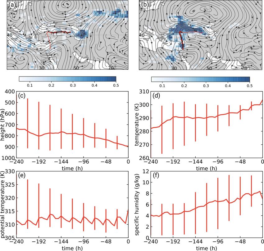
136                                                                      A. Hochman et al.: A new view of heat wave dynamics

temperature. Alpert et al. (2004b) argued that July and Au-          Here, ϑ is the extremal index (Moloney et al., 2019), which
gust represent the midsummer months, in which the Persian            we calculate using the Süveges maximum likelihood estima-
trough occurs on more than 9 d out of 11 d on average. For           tor (Süveges, 2007), and u and σ are parameters of the distri-
additional details on the computation of the CSI index and its       bution, which depend on the chosen ξ . The local dimension
evaluation, the reader is referred to Saaroni et al. (2017).         is then obtained as follows:
                                                                                  1
2.3    Dynamical systems metrics                                     d (ξ ) =          .                                          (5)
                                                                                σ (ξ )
We view the atmosphere as a chaotic dynamical system and
leverage a recently developed method combining extreme               Persistence is given by
value theory with Poincaré recurrences (Lucarini et al., 2016;                      1t
Faranda et al., 2017a) to estimate the dynamical properties          θ −1 (ξ ) =          ,                                       (6)
                                                                                   ϑ (ξ )
of atmospheric states. The temporal evolution of the atmo-
sphere can be represented as a long trajectory in a suitably         where 1t is the time interval between successive time steps
defined phase space. When we use temporally discretized              in our dataset. In practice, we choose each SLP map in the
data, such as reanalysis data, we are effectively sampling this      dataset in turn as state of interest ξ , which enables us to ob-
trajectory with a given time period, for example 6 or 24 h. An       tain a value of d and θ −1 for each time step in our dataset.
example would be analyzing daily latitude–longitude maps                In practical terms, d reflects the geometry of the trajecto-
of sea level pressure (SLP) over the eastern Mediterranean           ries in a small region (neighborhood) of the system’s phase
(technically a special Poincaré section of the full dynamics):       space around the state of interest. It is, therefore, related to
each 2-D map corresponds to a single point along the afore-          the number of active degrees of freedom that the system can
mentioned trajectory, for which we seek to compute instan-           explore about the state. In other words, it provides informa-
taneous (in time) and local (in phase space) properties. We          tion on the way the system evolves around the state of in-
specifically consider two metrics, which describe instanta-          terest, and a higher d will correspond to a less predictable
neous atmospheric states: the local dimension d and the per-         evolution of the system. The persistence θ −1 quantifies how
sistence θ −1 . In order to compute the local dimension and          long the system resides in the neighborhood of the state of
persistence for a given state of interest ξ , which in our exam-     interest. An infinite persistence implies a fixed point of the
ple would correspond to a specific SLP map in our dataset            system, such that all successive time steps bring no change to
for a dynamical system with trajectory x(t), we first define         the state of the system. At the opposite end of the spectrum,
logarithmic returns as follows:                                      θ −1 = 1 corresponds to a nonpersistent state of the dynamics.
                                                                     The dynamical systems persistence tends to be very sensitive
g (x (t) , ξ ) = − log (dist (x (t) , ξ )) ,                  (2)
                                                                     to small changes in the state of the system. In atmospheric
where dist is the Euclidean distance between two vectors.            sciences, persistence is often computed as the residence time
Thus, we define g such that it is large when the system is in        of the atmosphere within a given cluster of states. For exam-
states close to ξ and small when the system is in states far         ple, when computing the persistence of weather regimes, one
from ξ . In other words, g is large whenever the SLP map on          usually counts how long the atmosphere remains within one
a given day resembles the SLP map of the day corresponding           given weather regime cluster. However, there are typically a
to the state of interest ξ .                                         small number of clusters, such that each one contains a rela-
   We next consider all cases in which g exceeds a high              tively large fraction of the total number of time steps within
threshold s(q, ξ ), where q is a high quantile of the series g it-   the dataset. In our case, we define recurrences based on a
self. Here, we select q to be the 98th percentile of g. For these    high threshold such that only a small fraction of time steps
cases, which correspond to days whose SLP map is very sim-           within our dataset qualify as recurrences. Thus, by design,
ilar to that of ξ , we can then define exceedances as                θ −1 is more sensitive to small changes in the atmosphere than
                                                                     the conventional definition of persistence of weather regimes.
u (t, ξ ) = g (x (t) , ξ ) − s (q, ξ ) .                      (3)    The two are, nonetheless, related, and relative differences in
                                                                     θ −1 often reflect relative differences in more conventional at-
Given g above the threshold, we compute how far g is                 mospheric persistence metrics (Hochman et al., 2019).
above the threshold. The cumulative probability distribution            The above derivations hold under a specific set of con-
F (u, ξ ) of these exceedances converges to the exponential          ditions, which are seldom satisfied by climate, or indeed
member of the generalized Pareto distribution (GPD; Freitas          any real-world datasets – such as having infinitely long
et al., 2010; Lucarini et al., 2012). In other words, given a        time series. However, there are both formal (Caby et al.,
sufficiently long series of SLP maps, we know that the ex-           2020) and empirical (Messori et al., 2017; Buschow and
ceedances u computed from these maps obey the following:             Friedrichs, 2018) results, which support the application of

                                )
                                                                    this framework to natural data. In particular, Buschow and
                    −ϑ(ξ ) σu(ξ
                             (ξ )
F (u, ξ ) ' e                           .                     (4)    Friederichs (2018) have shown that d successfully reflects

Earth Syst. Dynam., 12, 133–149, 2021                                                         https://doi.org/10.5194/esd-12-133-2021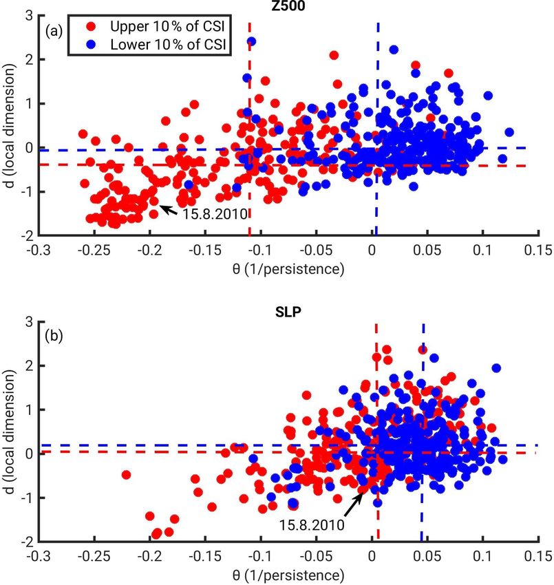
A. Hochman et al.: A new view of heat wave dynamics                                                                            137

the dynamical characteristics of the atmosphere even for
datasets where the universal convergence to the exponential
member of the GPD is not achieved. Messori et al. (2017)
further showed that the persistence estimates for atmospheric
data issuing from the Süveges estimator are very stable un-
der bootstrap resampling of the intra- and inter-cluster times
(i.e., the residence times of the trajectory within and outside
the neighborhood of the state of interest). For more details on
the estimation of the dynamical systems metrics, the reader
is referred to Lucarini et al. (2016) and Faranda et al. (2017a,
2019a).
   The dynamical systems perspective has been fruitfully
applied to a range of geophysical and other datasets (e.g.,
Faranda et al., 2019b, c; Brunetti et al., 2019; Faranda et al.,
2020; Hochman et al., 2020b; De Luca et al., 2020a; Pons et
al., 2020). It has also been explicitly shown that d and θ −1
can offer an objective characterization of synoptic systems
over different geographical regions, including the Mediter-
ranean (Hochman et al., 2019; De Luca et al., 2020b), the
North Atlantic (Faranda et al., 2017a; Messori et al., 2017;
Rodrigues et al., 2018) and the full Northern Hemisphere
(Faranda et al., 2017b). In this study, we compute d and θ −1
for daily and 6-hourly 500 hPa geopotential height (Z500)
and SLP fields from the NCEP/NCAR Reanalysis, over the
eastern Mediterranean, placing Israel in the middle of the do-
main (27.5–37.5◦ N, 30–40◦ E; Fig. 1). To understand the dif-
ferences between heat waves and cool days, we analyze both
the CDFs (cumulative distribution functions) and the mean
temporal evolution of the two groups of days in terms of d
and θ −1 . The Wilcoxon rank-sum (comparing the medians)
and Kolmogorov–Smirnov (comparing the CDFs) tests are              Figure 1. Mean sea level pressure (SLP, in hPa, white contours)
used for estimating the differences between the upper and          and 500 hPa geopotential height (Z500, in m, colored shading) for
lower 10 % of CSI days at the 5 % significance level. A boot-      the 10 % of days with the highest (heat waves) and lowest (cool
strap sampling test with 104 samples is used to evaluate the       days) climatic stress index (CSI) values: (a) heat wave days mean
95 % confidence intervals of the mean temporal evolutions.         composite; (b) cool days mean composite; (c) heat waves minus
   Previous studies have shown that the dynamical systems          cool days.
metrics d and θ −1 have a strong seasonal cycle (Faranda et
al., 2017a, b; Rodrigues et al., 2018; Hochman et al., 2020a).
Thus, we remove the seasonal cycle before comparing the            casts offer an efficient way of estimating uncertainty by com-
various events. As we are comparing individual days/events         puting the ensemble spread. This is quantified by estimat-
during different parts of the summer season, it is better to       ing the standard deviation between ensemble members. The
de-seasonalize the metrics in order to study the anomalies.        spread can be taken as an indicator of practical predictability:
In other words, we test whether heat waves are synoptically        in a perfect ensemble, a small spread would generally indi-
and dynamically unusual with respect to the cool days in the       cate that we can determine the future weather with a good
same part of the season. The seasonal cycle is estimated by        degree of confidence, whereas a large spread would point to-
averaging the metrics for a given time step (e.g., 15 August       wards a larger uncertainty (e.g., Buizza, 1997). This type of
at 12:00 UTC) over all years, repeating this for all time steps    approach is commonly used when investigating atmospheric
within the year and ultimately smoothing the series with a         predictability (e.g., Hohenegger et al., 2006; Ferranti et al.,
30 d moving average.                                               2015), although it does have limitations (e.g., Whitaker and
                                                                   Lough, 1998; Hopson, 2014).
2.4   Forecast spread and skill
                                                                      An additional frequently used forecast diagnostic is the
                                                                   absolute error, which provides a measure of forecast skill.
To obtain an ensemble forecast, a set of numerical forecasts       The correlation between the ensemble spread and skill of
are performed with either different initial conditions, and/or     the NWP model indicates the extent to which the ensemble
perturbation of physical parameterizations. Ensemble fore-         can be used to provide an a priori estimate of the practical

https://doi.org/10.5194/esd-12-133-2021                                                Earth Syst. Dynam., 12, 133–149, 2021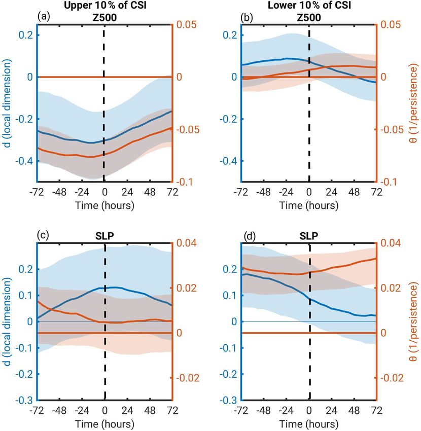
138                                                                       A. Hochman et al.: A new view of heat wave dynamics

predictability of the atmospheric configuration that we are         to about 720 m. Therefore, this can be considered a reason-
considering. Here, we use the homogeneous station archive           able choice.
mentioned in Sect. 2.1 above as ground truth to estimate the           The trajectories are calculated from 6-hourly ERA-Interim
forecasts’ absolute error. In order to remove biases due to to-     data and remapped to a 1◦ regular latitude–longitude grid.
pographic differences between the model and the stations, the       Thus, the analyzed wind field does not resolve sub-grid-scale
GEFS reforecast gridded data are bilinearly horizontally in-        processes, such as Lagrangian transports due to small con-
terpolated to the location of the stations. The bias computed       vective cells. Also, vertical motion associated with short-
over the whole period is then removed for each station.             lived convection between two time steps is not accounted for.
   The GEFS reforecasts are initialized at 00:00 UTC and are        Still, for a climatological investigation, which is the focus of
available at 3 h intervals. As our analysis focuses on heat         this study, the trajectory calculation is a suitable diagnostic.
waves, we estimate the spread and skill for maximum tem-
perature and SLP at a lead time of 69 h, and the maximum
                                                                    3     Results
temperature is defined between 45 and 69 h. Given the 3 h
interval of the forecast data, bearing in mind that each sta-       3.1    Dynamics of heat waves over the eastern
tion’s maximum temperature is recorded between 20:00 and                   Mediterranean
20:00 UTC of the next day, this time window roughly cor-
responds to the definition of maximum temperature for the           We first analyze the differences between heat waves (upper
station data. As the dynamical systems metrics offer infor-         10 % of CSI values) and cool days (lower 10 % of CSI val-
mation on the temporal evolution of the atmosphere in the           ues). From an atmospheric dynamics’ standpoint, the main
neighborhood of a given reference state, we argue that using        difference between the two groups is that heat wave days
the time of forecast initialization as the temporal coordinate      are associated with an upper-level ridge, whose center is lo-
when plotting spread and error is most indicative for com-          cated in the southeastern part of the study region (Fig. 1a),
paring the dynamical systems and numerical forecasts. In the        whereas cool days are associated with an upper-level trough,
Supplement, we also plot the spread and skill for the fore-         whose center is located at the northwestern part of the study
casts initialized 69 h before the marked time. Thus, the plots      region (Fig. 1b). The SLP patterns are quite similar in both
in the main text show forecast initialization times, whereas        groups, but the heat waves show lower SLP in the southwest
those in the Supplement show the forecast valid times. Statis-      and a higher SLP in the northeast compared with the cool
tical inference is accomplished by the same tests mentioned         days sample (Fig. 1c). This implies stronger pressure gradi-
in Sect. 2.3.                                                       ents in the cool days’ subgroup, leading to enhanced cool air
                                                                    advection from the Mediterranean Sea inland, in compari-
2.5   Air parcel tracking
                                                                    son to the heat wave days. Furthermore, the abovementioned
                                                                    pattern reveals that the large-scale configuration is an impor-
In order to identify typical pathways of air masses lead-           tant factor in the generation of a heat wave over the eastern
ing to situations with high and low CSI values, 10 d back-          Mediterranean. The backward trajectory air parcel analysis
ward trajectories are computed using the Lagrangian analysis        illustrates that the flow preceding an extreme heat wave has a
tool (LAGRANTO; Wernli and Davies, 1997; Sprenger and               roughly meridional orientation when traveling over the east-
Wernli, 2015). The reader is referred to Fig. 2 in Sprenger         ern Mediterranean and originates over the European conti-
and Wernli (2015) for a schematic overview of the typical           nent (Fig. 2a). On the other hand, the air parcels for cool
steps taken to compute trajectories. The tracking of temper-        days often originate over the Atlantic and take a more zonal
ature and potential temperature along the trajectory further        pathway across the eastern Mediterranean (Fig. 2b). The ini-
allows for the quantification of the contribution of adiabatic      tial potential temperature of the heat wave air masses is about
and diabatic processes to the anomalous temperatures. The           7 K higher than that for the cool days (Fig. 2e). The differ-
vertical and horizontal wind components required for the tra-       ences in potential temperature between the two groups can
jectory computations are acquired from the ERA-Interim re-          mainly be attributed to the more continental origin of the
analysis (Sect. 2.1; Dee et al., 2011). The trajectories are ini-   air parcels for the heat waves: these air parcels potentially
tialized at 12:00 UTC from fixed points in the whole study          transport warmer air masses that descend on their path to the
region on the first day of a heat wave or cool days (Fig. 1).       target region. Their descent, which is stronger than for cool
In order to analyze the near-surface air masses, i.e., those re-    days (Fig. 2c), is accompanied by a temperature increase of
lated to the hot and cool conditions, we consider trajectories      more than 25 K during the 10 d period (Fig. 2d). The poten-
that are initialized between the surface and 90 hPa above the       tial temperature remains nearly constant until the final stages
surface. According to recent studies, the planetary bound-          of the descent except for the diurnal cycle (Fig. 2e). Thus, we
ary layer height in Israel during summer is ∼ 600–900 m             conclude that the extreme heat is related to an adiabatic de-
above the surface (Uzan et al., 2016, 2020). Assuming hy-           scent of the air parcels over the eastern Mediterranean rather
drostatic balance and, thus, a pressure decrease of approxi-        than to diabatic heating. In other words, the warm air parcels
mately 1 hPa every 8 m height difference, 90 hPa corresponds        are transported towards the eastern Mediterranean with the

Earth Syst. Dynam., 12, 133–149, 2021                                                  https://doi.org/10.5194/esd-12-133-2021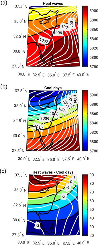
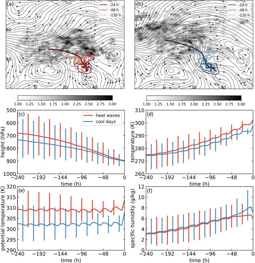
A. Hochman et al.: A new view of heat wave dynamics                                                                                      139

Figure 2. Median backward trajectory for (a) heat waves (upper 10 % of CSI) and (b) cool days (lower 10 % of CSI), with circles indicating
days (from 10 d before onset to onset). Gray shading shows the trajectory density 10 d before onset (number of trajectories per 1000 km2 ),
and contours show the trajectory density for the indicated time lags (5, 2 and 1 d before onset; contours denote a density of 20 trajectories
per 1000 km2 ). Streamlines of 800 hPa winds averaged between −5 and −1 d are included. The interquartile range of the trajectory positions
is shown using crosses for the different time lags. The median evolution of (c) pressure (hPa), (d) temperature (K), (e) potential temperature
(K) and (f) specific humidity (g kg−1 ) of air parcels is also shown. Heat waves are indicated in red, and cool days are shown in blue. The
interquartile range is plotted for the physical properties of the air parcels. A value of 0 h corresponds to the first day of CSI ≥ 90 % or
CSI ≤ 10 % and at 12:00 UTC.

governing westerlies rather than heated up locally over sev-             events that the portion of terrestrial back-trajectories for cool
eral days. This supports the findings of Harpaz et al. (2014),           days reaches a minimum and is much lower than for heat
who argued that extreme summer heat waves over the east-                 waves (Fig. S2).
ern Mediterranean are mostly regulated by midlatitude dis-                  From a dynamical systems point of view, the upper and
turbances rather than by the Asian monsoon, as previously                lower 10 % of CSI also exhibit substantial differences. Fig. 3
proposed by Ziv et al. (2004). An additional important dif-              shows a phase plane diagram for d and θ computed on Z500
ference between the two sets of CSI events is that, unlike               and SLP for the heat waves and cool days. θ is significantly
for the heat waves (Fig. 2a, f), the specific humidity of the            lower at both levels for heat waves with respect to cool days,
cool days increases by 2 g kg−1 around t = −48 h, due to                 i.e., the former are generally more persistent systems. Statis-
the longer stretch that the latter air parcels follow over the           tically significant differences in the median local dimensions
Mediterranean Sea (Fig. 2b, f) and perhaps some enhanced                 (d) of the two groups are found only for the Z500 variable,
convection, which our analysis does not account for. Indeed,             for which the heat waves typically display a lower local di-
comparing the portion of terrestrial back-trajectories for heat          mension (d) than the cool days (Fig. 3a). The clear separa-
waves and cool days (Fig. S2) suggests that for most of the              tion between the two groups, especially at the upper level
time they are quite similar. It is only 72–24 h prior to the             (cf. Fig. 3a and b) correlates well with the atmospheric dy-

https://doi.org/10.5194/esd-12-133-2021                                                       Earth Syst. Dynam., 12, 133–149, 2021
140                                                                       A. Hochman et al.: A new view of heat wave dynamics

Figure 3. A phase plane diagram for the upper and lower 10 % of       Figure 4. The average temporal evolution of the dynamical sys-
CSI daily values (heat waves in red and cool days in blue). The de-   tems metrics (d and θ ) for heat wave (upper 10 % of CSI) and
seasonalized dynamical systems metrics (d and θ ) were computed       cool day (lower 10 % of CSI) events. The dynamical systems met-
for (a) Z500 and (b) SLP. Dashed lines represent the median values    rics were computed for (a, b) Z500 and (c, d) SLP. The events are
of d and θ . The 15 August 2010 is indicated by the black arrows.     centered (0 h) on the first day of CSI ≥ 90 % or CSI ≤ 10 % and at
                                                                      12:00 UTC. A 95 % bootstrap confidence interval is plotted (shad-
                                                                      ing).
namics’ viewpoint, which also shows more pronounced dif-
ferences at Z500 (Fig. 1). This points to the importance of
using different variables at different pressure levels to obtain      evolutions. Cool days are characterized by higher positive
a comprehensive picture of the dynamics of heat waves.                anomalies of d and θ in the days preceding the event. The
   Figure 4 displays the average temporal evolution of d and          buildup to this type of event is characterized by an increase
θ during the selected events, again computed for Z500 and             in θ (decrease in persistence) and a decrease in d (decrease
SLP. Zero on the x axis denotes the first day of the event at         in active degrees of freedom; Fig. 4d). The cool days also ap-
12:00 UTC, whereas a value of zero on the y axis implies that         pear to have a more coherent evolution (lower spread around
the events are not different from the climatology of the days         the mean) than the heat waves for SLP.
they occurred in. Substantial differences are found between              Thus, the differentiation between the two samples is more
the time evolutions of the upper and lower 10 % of the CSI            pronounced when computing the metrics on Z500 than on
events. For Z500, the temporal evolution of d and θ for heat          SLP (Fig. 4), as also shown in the daily distributions (Fig. 3).
waves are in phase with each other and show a minimum with            Moreover, the variability in the temporal evolution of the
below climatology values in the 24 h preceding the event on-          dynamical systems metrics is smaller in Z500 than in SLP
set (Fig. 4a). While there is still a considerable spread around      (Fig. 4). This points to (i) coherent, and very different, upper-
the mean, even the upper bounds of our confidence intervals           level conditions, which engender the two sets of CSI days
are well below zero in the buildup to the events. Instead, cool       as well as (ii) a comparatively wide range of possible near-
days display weak positive anomalies of d and θ , but these           surface patterns leading to severe heat waves. The latter may
are almost never significantly different from zero (Fig. 4b).         be explained by the fact that, given initially warm upper-
The dynamical systems metrics computed on SLP provide                 level air parcels and upper-level subsidence leading to rapid
a completely different picture: heat waves typically display a        adiabatic warming, the occurrence of a heat wave is then
weak above climatology d, which increases towards the event           relatively insensitive to the details of the surface conditions
onset and then decreases (Fig. 4c). θ displays a slightly be-         (e.g., Baldi et al., 2006; Harpaz et al., 2014). Our general un-
low climatology persistence (i.e., positive anomalies) and de-        derstanding of the synoptic conditions at surface levels fur-
creases towards the event onset (Fig. 4c). However, the very          ther suggests that the delicate interplay between the Persian
large spread in the composite evolution, in particular in d,          trough and subtropical high systems (Alpert et al., 1990) may
suggests some caution in overinterpreting the details of these        contribute to the large spread of both heat waves and cool

Earth Syst. Dynam., 12, 133–149, 2021                                                    https://doi.org/10.5194/esd-12-133-2021
A. Hochman et al.: A new view of heat wave dynamics 141
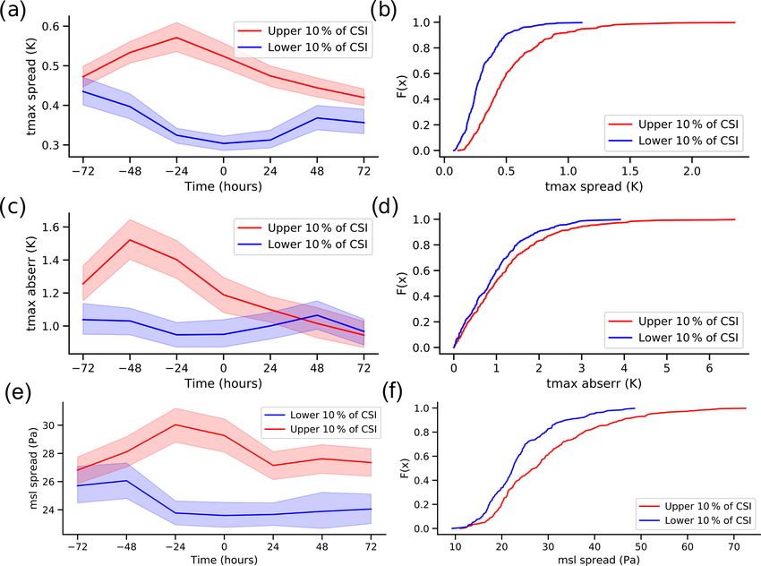
Figure 5. Forecast spread and skill for heat waves (upper 10 % of CSI) and cool days (lower 10 % of CSI). The lines show the mean
temporal evolution of the ensemble model spread for Tmax (a), SLP (e) and the absolute error for Tmax (c) of forecasts with a lead time
of 69 h, initialized at different time lags with respect to the events, calculated every 24 h. The events are centered (0 h) on the first day of
CSI ≥ 90 % or CSI ≤ lower 10 % and at 12:00 UTC. The CDFs of the mean ensemble forecast model spread for Tmax (b), SLP (f) and the
absolute error of Tmax (d) for the forecasts with a lead time of 69 h initialized at 00:00 UTC. A 95 % bootstrap confidence interval is shown
using shading for the temporal evolution plots (a, c, e). The plots are displayed for the time of forecast initialization (see Sect. 2.4).
days regarding the dynamical systems metrics computed on 3.2 Analysis of the mid-August 2010 heat wave over the
SLP. eastern Mediterranean
We next analyze numerical ensemble forecasts from the
GEFS reforecast dataset for both sets of events. Substantial The mid-August 2010 heat wave over the eastern Mediter-
differences are again found between the two groups (Fig. 5). ranean was a severe event, which lies in the upper 0.3 % of
Both the ensemble spread and the absolute error are signif- the CSI distribution. A detailed analysis of the heat wave
icantly higher for heat waves than for cool days (Fig. 5). highlights both similarities and differences with the clima-
The model spread and absolute error increase before the on- tology of the heat wave days (Sect. 3.1). The Z500 and SLP
set of the heat wave and peak at around 24–48 h negative patterns for 15 August 2010 are comparable with the average
lags (Fig. 5). This pattern stands in stark contrast to the tem- configuration of a heat wave, but they show a stronger upper-
poral evolution of d computed on Z500 (cf. Figs. 5a, c, e level ridge and meridionally oriented isobars (cf. Figs. 6a
and 4a), but it somewhat resembles the evolution of d com- and 1a). From a dynamical systems point of view, the 2010
puted on SLP, albeit with a ∼ 24 h shift in time (cf. Figs. 5e heat wave was also an uncommon extreme, especially for the
and 4c). Such a shift may be explained by the fact that the metrics computed on Z500. The dynamical systems metrics’
spread and skill of the ensemble forecasts are computed ev- anomalies computed on this field range between −0.9 and
ery 24 h, whereas the dynamical systems metrics are instan- −1.4 for d and between −0.14 and −0.2 for θ (Fig. 6b). This
taneous in time (local in phase space) and computed from 6- situates the heat wave in the lower 10 % of the respective dis-
hourly data. The reforecasts computed for the individual sta- tributions (see also red dots in Fig. 3a). During its evolution,
tions (not shown) resemble the average forecast spread and the event displays an increase in both d and θ computed on
skill (Fig. 5). The corresponding plots for forecast valid time Z500 and a decrease (increase) in θ (d) computed on SLP
(see Sect. 2.4) are provided in Fig. S3. (Fig. 6b, c). Whereas the Z500 d and θ evolution is roughly
comparable to that identified for heat wave days (cf. Figs. 4a
and 6b), the SLP d and θ evolutions show profound differ-
ences. This may simply reflect the larger spread in dynam-
https://doi.org/10.5194/esd-12-133-2021 Earth Syst. Dynam., 12, 133–149, 2021142 A. Hochman et al.: A new view of heat wave dynamics
tween −10 and −5 d prior to the event, the majority of air
parcels were transported in an easterly flow on the southern
flank of an anticyclone located over Russia. Thus, air parcels
came from the Zagros Plateau of northern Iran, rather than
from central Europe as in the climatology (cf. Figs. 7a, b
and 2a). Indeed, Zaitchik et al. (2007) argued that the Za-
gros Plateau has a strong influence on extreme summertime
heat waves over the eastern Mediterranean. Here we show
that the anticyclonic wave breaking of the blocking regime
over Russia, which interestingly is related to the decay phase
of the Russian 2010 heat wave (Quandt et al., 2019), played
an important role in transporting the warm air masses from
northern Iran towards the eastern Mediterranean and Israel
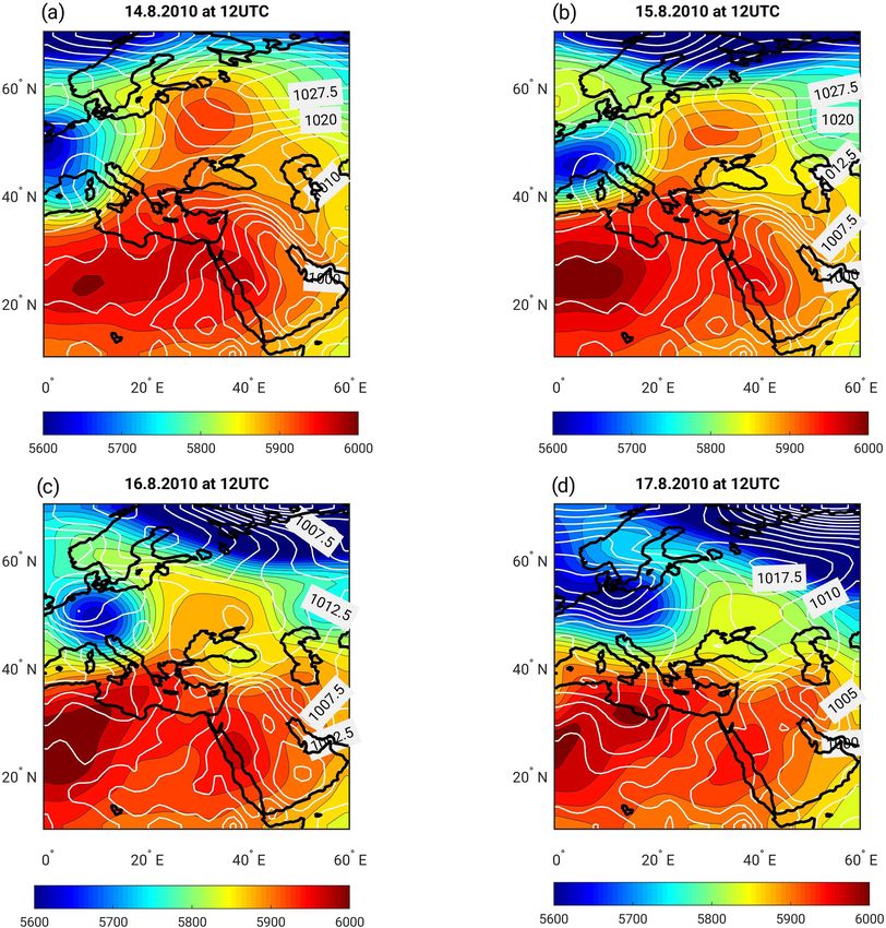
(Figs. 7a, b and 8). This is realized through the trough
east of the blocking ridge centered over European Russia,
which is tilted southwest–northeast and advected westward
(Fig. 8b, c, d, Davini et al., 2012; Quandt et al., 2019). For
the last 5 d prior to the heat wave (Fig. 7b), the parcel’s
trajectories more closely resemble the climatology of heat
waves (Fig. 2a). Reflecting the different advection pathways,
the initial potential temperature and temperature of the air
parcels are about 2 and 7 K higher than the climatology of
heat waves, respectively (cf. Figs. 7d, e and 2d, e). Accord-
ingly, the hot air masses in the mid-August 2010 heat wave
are transported to the eastern Mediterranean and undergo adi-
abatic heating, rather than being heated up locally. This is in
line with the climatology discussed in Sect. 3.1 as well as
Figure 6. A dynamical systems analysis for the mid-August 2010 heat waves in other parts of the world (e.g., Bieli et al., 2015;
heat wave. (a) SLP (white contours, in hPa) and Z500 (shading, Quinting and Reeder, 2017; Zschenderlein et al., 2019).
in m) on 15 August 2010 at 12:00 UTC. The dynamical systems Figure 9 shows the temporal evolution of the forecast
metrics’ (d and θ ) temporal evolution centered on 15 August 2010 spread and skill for the mid-August 2010 heat wave com-
at 12:00 UTC (0 h) computed on (b) Z500 and (c) SLP. pared to the heat wave climatology. Throughout the lead-up
and early phases of the event, the forecast displays a lower
spread and error than for other heat waves. A large decrease
ical systems properties across the different heat waves for in the practical predictability occurs as the event develops,
SLP than for Z500, which is likely to be partially modulated i.e., an increase in the spread and decrease in the skill for
by interactions between the surface and the atmosphere. Nat- maximum temperature (Fig. 9a, b). This mirrors the increase
urally, these interactions predominantly affect the lowermost in d and θ computed on Z500 and for d computed on SLP
parts of the troposphere. We further hypothesize that differ- (cf. Figs. 9a, b with Fig. 6b, c). Indeed, the decay phase of
ences between the single case and the climatology may be the Russian heat wave was characterized by low practical
related to the relatively small day-to-day variations during predictability (Matsueda, 2011), which may have influenced
summer over the eastern Mediterranean, which make it chal- the predictability over the eastern Mediterranean. However,
lenging to depict the exact onset of a heat wave. Indeed, when it should be noted that the spread computed on the maximum
comparing the climatology of the temporal evolution of d and temperature for the mid-August 2010 heat wave does not cor-
θ for Z500 (Fig. 4a) with the single case (Fig. 6b), it is rela- relate well with the spread computed on SLP (cf. Fig. 9a
tively easy to see that there is an increase in both d and θ as with c). Moreover, some striking differences are displayed
the heat wave develops. On the other hand, when comparing between the ensemble forecast of this single event and the
the temporal evolution of d and θ for SLP (Figs. 4c with 6c), climatology of forecasts for heat waves. These discrepancies
one can see that depicting the exact time that the heat wave may be related to the fact that we are analyzing a single event,
starts is very important for comparison. In both Figures, d whose error may not reflect the practical predictability of the
increases and θ decreases at some point in the chosen time atmosphere even for a perfect ensemble (e.g., Whitaker and
window, but the timing of these trends is shifted between the Lough, 1998; Buizza et al., 2005; Hopson 2014). The cor-
climatology (Fig. 4c) and the single case (Fig. 6c). responding plots for forecast valid time (see Sect. 2.4) are
The 2010 heat wave was also uncommon in terms of the provided in Fig. S4.
large-scale flow and Lagrangian trajectories (Fig. 7). Be-
Earth Syst. Dynam., 12, 133–149, 2021 https://doi.org/10.5194/esd-12-133-2021A. Hochman et al.: A new view of heat wave dynamics 143
Figure 7. Backward trajectory air parcel tracking for the mid-August 2010 heat wave initialized on 15 August 2010 at 12:00 UTC with
(a) circles indicating days (from −10 to −6 d before 15 August 2010 at 12:00 UTC), gray shading indicating trajectory density 10 d before
onset (number of trajectories per 1000 km2 ) and streamlines of 800 hPa wind (averaged between −10 and −6 d before 15 August 2010 at
12:00 UTC). Panel (b) is the same as panel (a) but for −5 to −1 d and a trajectory density of 5 d before onset. The median evolution of
(c) height (hPa), (d) temperature (K), (e) potential temperature (K) and (f) specific humidity (g kg−1 ) of the tracked air parcels is also shown.
The interquartile range is plotted for the physical properties of the air parcels. A value of 0 h corresponds to 15 August 2010 at 12:00 UTC.
4 Summary and conclusions trinsic predictability of heat waves over the eastern Mediter-
ranean is highest, i.e., low local dimension (d) and high per-
sistence (low θ ), in the 24 h preceding the onset of the event
Heat waves are a major weather-related hazard, especially
and lowest in the decay phase of the event. Indeed, Lucarini
in an era of rapid climate change. We define heat waves over
and Gritsun (2020) recently argued that atmospheric block-
the eastern Mediterranean according to a state-of-the-art ‘cli-
ing over the Atlantic also displays such characteristics. The
matic stress index’ (CSI; Saaroni et al., 2017), developed
persistent upper-level ridge that characterizes the heat waves
specifically for the region’s summer weather conditions. We
may explain the high intrinsic predictability during the on-
use a combination of dynamical systems theory, numerical
set phase. The dynamical systems metrics computed on SLP
weather forecasts and air parcel back-trajectories to investi-
show a different temporal evolution to their Z500 counter-
gate the evolution and predictability characteristics of heat
parts, emphasizing the different characteristics of the atmo-
waves (high CSI) and cool days (low CSI) for the region.
spheric flow at the different vertical levels. Specifically, there
The main conclusions are as follows: significant differ-
is a very large spread across different heat wave events. We
ences are found between heat waves and cool days from
argue that this may be associated with the delicate interplay
both a dynamical systems and numerical weather prediction
between the subtropical high and the Persian trough at sur-
perspectives. Heat waves show relatively low practical pre-
face levels (Alpert et al., 1990), which can lead to a range of
dictability (large model spread and low skill) in the ensem-
different SLP configurations all leading to a heat wave. This
ble reforecast dataset used here, in spite of the relatively sta-
may further be reasonably attributed to the interactions be-
ble flow characteristics (high intrinsic predictability) com-
tween the land and/or sea surface and the atmosphere, which
pared with the cool days. When considering Z500, the in-
https://doi.org/10.5194/esd-12-133-2021 Earth Syst. Dynam., 12, 133–149, 2021144 A. Hochman et al.: A new view of heat wave dynamics Figure 8. The large-scale evolution of SLP (white contours, in hPa) and Z500 (shading, in m) for the mid-August 2010 heat wave: (a) 14 Au- gust 2010 at 12:00 UTC, (b) 15 August 2010 at 12:00 UTC, (c) 16 August 2010 at 12:00 UTC and (d) 17 August 2010 at 12:00 UTC. mainly influence the lower parts of the troposphere. How- by underscoring how the parcels, which contributed to the ever, it is important to note that in many – albeit certainly heat wave, were warmer than those of the climatology of not all – cases these interactions influence the atmosphere heat waves as early as 10 d prior to the event. Interestingly, at timescales longer than those we consider in our analysis the onset of the heat wave over the eastern Mediterranean (e.g., Entin et al., 2000), and they can act as a seasonal- was related to the decay phase of the Russian heat wave scale preconditioning to extremely high summer tempera- (Quandt et al., 2019), and we conclude that the anticyclonic tures (Zampieri et al., 2009; Zittis et al., 2014). Rossby wave breaking over Russia contributed to the onset Based on the Lagrangian air parcel analysis, we conclude of the eastern Mediterranean heat wave. The 2010 heat wave that the physical processes governing eastern Mediterranean showed both differences and similarities to other heat waves, summer heat waves relate to adiabatic descent of the air highlighting the range of possible atmospheric and dynam- parcels over the region rather than diabatic heating, in agree- ical developments leading to high CSI values. This is com- ment with previous findings (e.g., Harpaz et al., 2014). In pounded by the general difficulty of analyzing the life cycle other words, the air parcels are transported horizontally and of heat waves, as there is little agreement as to what exactly a vertically towards the eastern Mediterranean with the gov- heat wave is and when it starts and ends (Shaby et al., 2016). erning westerlies rather than heated up locally over consec- We conclude that the instantaneous dynamical systems utive days. We further conclude that the origin of the air metrics of local dimension (d) and persistence (θ −1 ) pro- parcels over land in the days before the onset of a heat wave vide complementary information on extreme summer heat plays an important part in its generation. waves compared with the conventional analysis of numeri- A detailed analysis of the record-breaking mid-August cal weather forecasts. The discrepancy between the practical 2010 heat wave provides further insights in this respect and the intrinsic predictability of the heat waves reflects this Earth Syst. Dynam., 12, 133–149, 2021 https://doi.org/10.5194/esd-12-133-2021
A. Hochman et al.: A new view of heat wave dynamics                                                                                          145

                                                                            correlated for maximum temperature, but this is not a univer-
                                                                            sal rule. For example, the mid-August 2003 heat wave had
                                                                            a very low spread (Tmax spread = 0.2 K; cf. Fig. 5b) and an
                                                                            above average error (Tmax absolute error = 1.1 K; cf. Fig. 5d).
                                                                            However, both d and θ computed on Z500 display a strong
                                                                            increase (d = −1.7 to 0.3, θ = −0.2 to 0.1 over the consid-
                                                                            ered time window, not shown; cf. Figs. 4a and 6b), pointing
                                                                            to a decrease in intrinsic predictability. In such cases, local
                                                                            dimension (d) and/or persistence (θ −1 ) trends that seem to
                                                                            contradict a low ensemble spread may serve as a warning of
                                                                            a potentially poor spread–skill relationship.
                                                                               As a caveat, the comparison of the practical and intrin-
                                                                            sic predictability still carries some interpretation challenges.
                                                                            Although the differences between the two can be partly as-
                                                                            cribed to the different characteristics of the two measures,
                                                                            they may also be subject to the shortcomings of the GEFS
                                                                            ensemble data. In particular, the spread of the GEFS ensem-
                                                                            ble data, as most NWP ensemble forecasts, does not always
                                                                            reflect the practical predictability of the atmospheric flow
                                                                            (e.g., Whitaker and Lough, 1998). Moreover, our interpre-
                                                                            tation of the dynamical systems metrics may also be imper-
                                                                            fect. Indeed, the metrics provide local information in phase
                                                                            space, whereas the spread and error of an ensemble forecast
                                                                            presumably reflect the longer-term evolution of the atmo-
                                                                            spheric flow. Similar interpretation challenges for the practi-
                                                                            cal versus intrinsic predictability have emerged when study-
                                                                            ing cold spells over the eastern Mediterranean (Hochman et
                                                                            al., 2020a).
                                                                               Notwithstanding these ongoing challenges, we believe that
Figure 9. Forecast spread and skill for the mid-August 2010 heat            the novel view presented here, which leverages a dynami-
wave, centered (0 h) on 15 August 2010 at 12:00 UTC (black line).           cal systems approach for diagnosing extreme weather events,
The mean temporal evolution of the ensemble model spread for                outlines an important avenue of research. We trust that it
Tmax (a), SLP (c) and the absolute error for Tmax (b) of forecasts          may be successfully applied to other regions and weather ex-
with a lead time of 69 h, initialized at different time lags with respect   tremes in the future.
to the event, computed every 24 h. The heat waves (upper 10 % of
CSI – red lines) are displayed for reference. A 95 % bootstrap con-
fidence interval for all heat waves is displayed (shading).                 Code availability. The code for computing the dynamical systems
                                                                            metrics is publicly available at https://www.lsce.ipsl.fr/Pisp/davide.
                                                                            faranda/ (Laboratoire des Sciences du Climat et de l’Environment,
complementarity. For example, we interpret a very persistent                2021), and code for computing backward trajectories is publicly
                                                                            available at https://iacweb.ethz.ch/staff/sprenger/lagranto/ (ETH
system as being intrinsically highly predictable, yet the nu-
                                                                            Zürich, 2021).
merical forecasts we analyze display larger spread and error
for the more persistent atmospheric configurations. In this
respect, having an a priori measure of the persistence of an
                                                                            Data availability. The paper and/or the Supplement contain or
atmospheric configuration from dynamical systems can be                     provide instructions to access all of the data needed to evaluate the
a useful complement to the numerical forecast. Specifically,                conclusions drawn in the paper. Additional data are available from
the practical predictability relies on the performance of a nu-             the corresponding author upon request.
merical forecast model. As such, it blends model and data
assimilation biases with the intrinsic characteristics of the
atmospheric flow. Moreover, even a perfect ensemble may                     Supplement. The supplement related to this article is available
not provide a good spread–skill relationship (Hopson, 2014).                online at: https://doi.org/10.5194/esd-12-133-2021-supplement.
That is, even a perfect ensemble may have a spread that does
not always reflect the actual forecast error (Whitaker and
Lough, 1998; Buizza, 1997). In the specific case of the heat                Author contributions. All authors contributed to the conceptual
waves that we analyze here, the spread and skill were well                  development of the study. AH and GM analyzed the data from a dy-

https://doi.org/10.5194/esd-12-133-2021                                                          Earth Syst. Dynam., 12, 133–149, 2021
You can also read