Labrador Sea subsurface density as a precursor of multidecadal variability in the North Atlantic: a multi-model study - CentAUR
←
→
Page content transcription
If your browser does not render page correctly, please read the page content below
Labrador Sea subsurface density as a
precursor of multidecadal variability in the
North Atlantic: a multi-model study
Article

Published Version

Creative Commons: Attribution 4.0 (CC-BY)

Open Access

Ortega, P., Robson, J. I. ORCID: https://orcid.org/0000-0002-
3467-018X, Menary, M., Sutton, R. T. ORCID:
https://orcid.org/0000-0001-8345-8583, Blaker, A., Germe, A.,
Hirschi, J. J.-M., Sinha, B., Hermanson, L. and Yeager, S.
(2021) Labrador Sea subsurface density as a precursor of
multidecadal variability in the North Atlantic: a multi-model
study. Earth System Dynamics, 12 (2). pp. 419-438. ISSN
2190-4987 doi: https://doi.org/10.5194/esd-12-419-2021
Available at http://centaur.reading.ac.uk/97692/

It is advisable to refer to the publisher’s version if you intend to cite from the
work. See Guidance on citing .

To link to this article DOI: http://dx.doi.org/10.5194/esd-12-419-2021

Publisher: European Geosciences Union
All outputs in CentAUR are protected by Intellectual Property Rights law,
including copyright law. Copyright and IPR is retained by the creators or other
copyright holders. Terms and conditions for use of this material are defined in
the End User Agreement .

www.reading.ac.uk/centaur

CentAUR

Central Archive at the University of Reading
Reading’s research outputs online
Earth Syst. Dynam., 12, 419–438, 2021
https://doi.org/10.5194/esd-12-419-2021
© Author(s) 2021. This work is distributed under
the Creative Commons Attribution 4.0 License.

             Labrador Sea subsurface density as a precursor of
               multidecadal variability in the North Atlantic:
                           a multi-model study
        Pablo Ortega1,2 , Jon I. Robson1 , Matthew Menary3 , Rowan T. Sutton1 , Adam Blaker4 , Agathe Germe4 ,
                    Jöel J.-M. Hirschi4 , Bablu Sinha4 , Leon Hermanson5 , and Stephen Yeager6,7
                       1 National   Centre for Atmospheric Science, University of Reading, Reading, UK
                                       2 Barcelona Supercomputing Center, Barcelona, Spain
                                          3 LOCEAN, Sorbonne Universités, Paris, France
                               4 National Oceanography Centre, European Way, Southampton, UK
                                              5 Met Office Hadley Centre, Exeter, UK
                                 6 National Center for Atmospheric Research, Boulder, CO, USA
              7 International Laboratory for High-Resolution Earth System Prediction, College Station, TX, USA

                                    Correspondence: Pablo Ortega (pablo.ortega@bsc.es)

                                Received: 1 November 2020 – Discussion started: 5 November 2020
                           Revised: 8 February 2021 – Accepted: 6 March 2021 – Published: 26 April 2021

       Abstract. The subpolar North Atlantic (SPNA) is a region with prominent decadal variability that has experi-
       enced remarkable warming and cooling trends in the last few decades. These observed trends have been preceded
       by slow-paced increases and decreases in the Labrador Sea density (LSD), which are thought to be a precursor
       of large-scale ocean circulation changes. This article analyses the interrelationships between the LSD and the
       wider North Atlantic across an ensemble of coupled climate model simulations. In particular, it analyses the
       link between subsurface density and the deep boundary density, the Atlantic Meridional Overturning Circulation
       (AMOC), the subpolar gyre (SPG) circulation, and the upper-ocean temperature in the eastern SPNA.
          All simulations exhibit considerable multidecadal variability in the LSD and the ocean circulation indices,
       which are found to be interrelated. LSD is strongly linked to the strength of the subpolar AMOC and gyre
       circulation, and it is also linked to the subtropical AMOC, although the strength of this relationship is model-
       dependent and affected by the inclusion of the Ekman component. The connectivity of LSD with the subtropics
       is found to be sensitive to different model features, including the mean density stratification in the Labrador
       Sea, the strength and depth of the AMOC, and the depth at which the LSD propagates southward along the
       western boundary. Several of these quantities can also be computed from observations, and comparison with
       these observation-based quantities suggests that models representing a weaker link to the subtropical AMOC
       might be more realistic.

1   Introduction                                                   across a range of different variables (Häkkinen and Rhines,
                                                                   2004; Holliday et al., 2020; Reverdin, 2010; Robson et al.,
The North Atlantic Ocean is a key component in Earth’s cli-        2018b). Basin-mean sea surface temperature (SST) over the
mate through, for example, its role in redistributing heat and     North Atlantic has also been observed to vary on multi-
in taking up excess heat and carbon from the atmosphere.           decadal timescales (Schlesinger and Ramankutty, 1994) and
It is also a region that has varied significantly in the past.     has been linked to a range of important climate impacts, in-
This is particularly true for the North Atlantic subpolar gyre,    cluding hurricane numbers and rainfall in monsoon regions
which has varied significantly on multidecadal timescales          (Knight et al., 2006; Monerie et al., 2019; Zhang and Del-

Published by Copernicus Publications on behalf of the European Geosciences Union.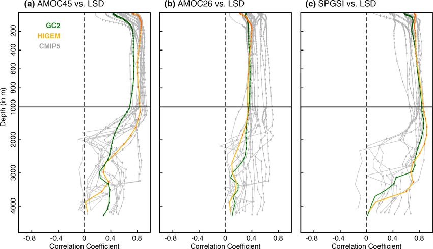
420                            P. Ortega et al.: Labrador Sea subsurface density and North Atlantic multidecadal variability

worth, 2006). The North Atlantic is also expected to change        son and Sutton, 2012; Ortega et al., 2017; Robson et al.,
significantly in the future due to the effects of climate change   2014, 2016). Observations show considerable decadal vari-
and consequently produce substantial climate impacts on the        ability in subsurface density anomalies; density anomalies in
surrounding regions (Sutton and Hodson, 2005; Woollings            the western SPNA and Labrador Sea between ∼ 1000 and
et al., 2012). On decadal timescales, it is the interaction be-    2500 m increased significantly, peaked in ∼ 1995, and subse-
tween natural variability and externally forced changes that       quently declined (Robson et al., 2016; Yashayaev and Loder,
will shape how the Atlantic region’s climate will evolve.          2016). Therefore, these density anomalies have been inter-
Therefore, in order to improve predictions of the North At-        preted as indicating that the AMOC peaked in the middle
lantic, it is imperative that we improve our understanding of      to late 1990s and then declined, consistent with the warm-
the processes that control decadal-timescale changes in this       ing and then cooling of the eastern SPNA (Hermanson et al.,
region.                                                            2014; Ortega et al., 2017; Robson et al., 2016). Time series of
   It has generally been thought that changes in the ocean         subsurface density anomalies in the western SPNA are also
circulation, particularly the Atlantic Meridional Overturning      consistent with other proxies for AMOC strength, including
Circulation (AMOC), have played a significant role in shap-        sea-level-based proxies (McCarthy et al., 2015; Sutton et al.,
ing the Atlantic multidecadal variability (AMV; Knight et al.,     2018), sediment based proxies (Thornalley et al., 2018), and
2005). In particular, changes in the strength of the AMOC          upper-ocean heat content fingerprints (Caesar et al., 2018;
and its related ocean heat transports have been shown to           Zhang, 2008). Furthermore, the decline in the AMOC sug-
control multidecadal internal variability in a range of cou-       gested by the above proxies is also consistent with the ob-
pled climate models (Danabasoglu, 2008; Dong and Sutton,           served AMOC decline at 26◦ N since 2004 (Smeed et al.,
2005; Jungclaus et al., 2005; Ortega et al., 2011, 2015). The      2018) and with the changes in the AMOC seen in ocean data
proposed mechanisms to explain the multidecadal variabil-          assimilation systems (Jackson et al., 2016, 2019). Therefore,
ity involve interplays between the North Atlantic Oscillation      there is confidence that large-scale changes in North Atlantic
(NAO), North Atlantic Deep Water (NADW) formation, the             Ocean circulation have occurred over the past few decades
boundary currents, the Gulf Stream and gyre circulations,          and that they have had a significant impact on upper-ocean
and the horizontal density gradients (e.g. Joyce and Zhang,        heat content.
2010; Polyakov et al., 2010; Ba et al., 2013; Nigam et al.,           Although there is consistency across proxies for AMOC
2018; Zhang et al., 2019). Changes in the AMOC and the             changes in the North Atlantic, there are considerable gaps in
wider ocean circulation have indeed been used to explain the       our understanding and major uncertainties to overcome. For
observed changes in the subpolar North Atlantic (SPNA) on          example, the development of subsurface density proxies has
decadal and longer timescales (Moat et al., 2019). In par-         been investigated so far with just a few models (Ortega et al.,
ticular, the SPNA underwent a rapid warming and salini-            2017; Robson et al., 2014). However, there is considerable
fication in the mid-1990s before a decadal-timescale cool-         spread across climate models in the simulations of AMOC
ing and freshening started in 2005, which is consistent with       mean state and variability (Reintges et al., 2017; Zhang and
decadal to multidecadal variability of the AMOC (Robson et         Wang, 2013) and also in the latitudinal coherence of AMOC
al., 2012, 2013, 2016). The recent cooling has been linked         anomalies (Li et al., 2019; Roberts et al., 2020; Hirschi et
to climate impacts over the continents, including heat waves       al., 2020), which might reflect different roles of deep den-
(Duchez et al., 2016), through an effect on the position of the    sity anomalies in the western SPNA for the AMOC, as well
jet stream (Josey et al., 2018). A long-term relative cooling of   as different interplays between the subpolar and subtropical
the SPNA since ∼ 1850 has also been attributed to a centen-        gyre contributions (Zou et al., 2020). Models also do not re-
nial weakening of the AMOC (Caesar et al., 2018; Rahm-             alistically resolve many key features of the AMOC, most no-
storf et al., 2015), an AMOC reduction that most CMIP6             tably the overflows, and this affects the subsurface stratifica-
model projections predict to continue in the future (Weijer        tion downstream and on the western boundary (Zhang et al.,
et al., 2020). However, a lack of direct observations of the       2011). Significant uncertainty also remains for other impor-
strength of the AMOC and the ocean circulation more gener-         tant processes. For example, it is not yet clear whether the re-
ally have hindered our ability to make a direct attribution of     cent changes in the SPNA are an ocean response to buoyancy
recent changes.                                                    forcing or whether mechanical wind forcing has shaped the
   In order to understand the aforementioned changes in            recent observed changes (Robson et al, 2016; Piecuch et al.,
the SPNA on multidecadal timescales many authors have              2017). Local surface fluxes are also likely to explain a signifi-
turned to indirect measurements of the AMOC. One partic-           cant proportion of the recent cooling (Josey et al, 2018). Sub-
ular proxy for AMOC strength that has received some focus          surface density anomalies are not just a proxy for the AMOC,
recently involves density anomalies at depth in the western        but also more generally for buoyancy-forced (or thermoha-
SPNA or Labrador Sea region. In climate models, density            line) circulation changes, including gyre changes (Ortega et
anomalies in the western SPNA are a key predictor of den-          al., 2017; Yeager, 2015). Finally, the AMOC variability is
sity anomalies further south on the western boundary and           also thought to respond to local wind forcing on a range of
hence of the AMOC strength via thermal wind balance (Hod-          timescales, especially at lower latitudes (Polo et al., 2014;

Earth Syst. Dynam., 12, 419–438, 2021                                                 https://doi.org/10.5194/esd-12-419-2021
P. Ortega et al.: Labrador Sea subsurface density and North Atlantic multidecadal variability                              421

Zhao and Johns, 2014), which could disrupt or “mask” the         represent the variability of the basin-wide AMOC cell and
influence of subsurface density anomalies as they propagate      to identify the models that can produce more reliable predic-
further south.                                                   tions and projections of the SPNA. For this, we will specif-
   There is also considerable uncertainty in how and where       ically assess the connection between subsurface density and
subsurface density anomalies are formed in the SPNA and          AMOC at high and low latitudes via the western boundary.
how they are related to the AMOC. In observations and mod-       Furthermore, we will determine whether models consistently
els, most water transformation associated with the AMOC          support an impact of AMOC changes on the SPNA upper-
occurs within the SPNA, particularly in the eastern SPNA         ocean temperatures and, if not, investigate why. Our primary
(Desbruyères et al., 2019; Grist et al., 2014; Langehaug et      aim is to provide, for the first time in a multi-model context,
al., 2012). However, decadal changes in subsurface density       a broad characterization of these relationships using consis-
anomalies in the western SPNA have often been linked to          tent analysis frameworks and tools, documenting the uncer-
buoyancy forcing and changes in deep convection in the           tainty. The reasons for the uncertainty in the relationships
Labrador Sea or to changes in the volume of Labrador Sea         will also be explored, establishing links to key model cli-
Water production (Yashayaev and Loder, 2016; Yeager and          matological properties that could eventually be exploited as
Danabasoglu, 2014). Many studies have also reported that         emergent constraints. We intentionally do not explore in de-
the basin-wide AMOC in ocean-only and coupled models is          tail how subsurface density anomalies are formed in these
sensitive to heat flux or buoyancy forcing in the Labrador       models and leave this for further study.
Sea (Kim et al., 2020; Ortega et al., 2011, 2017; Xu et al.,        The paper is organized as follows. Section 2 describes the
2019; Yeager and Danabasoglu, 2014). Indeed, idealized ex-       experiments and methods. Labrador Sea density and its link
periments have shown that persisting positive NAO phases         to the ocean circulation and the wider North Atlantic are ex-
can strengthen the AMOC by fostering deepwater formation         plored across the multi-model ensemble in Sect. 3. The char-
via increased surface cooling in the Labrador Sea, thus in-      acteristics of the intermodel spread in the previous relation-
ducing changes in the zonal density gradient (Delworth and       ships are explored in Sect. 4. Section 5 presents the main
Zeng, 2016; Kim et al., 2020) and thermal wind responses.        conclusions of this study and discusses its implications.
However, the real link between deep convection, deepwater
formation, and density anomalies at depth in the Labrador        2     Experiments and methods
Sea is complex and not fully understood (Katsman et al.,
2018). Observations suggest that very little water transforma-   Here we provide an overview and brief description of the
tion and deepwater formation actually occur in the Labrador      models used in this study and provide some statistical con-
Sea (Pickart and Spall 2007; Lozier et al., 2019). Indeed, re-   siderations for the intermodel comparison.
cently it has been shown that the Labrador Sea (i.e. OSNAP
west) has played a very minor role in the interannual vari-
                                                                 2.1    Experiment selection
ability observed so far across the whole OSNAP line (Lozier
et al., 2019), with the Irminger Sea playing a more dominant     For the multi-model analysis, we use the preindustrial con-
role. The Irminger Sea is a region that in some models con-      trol simulations (picontrol) from the fifth phase of the Cou-
trols the AMOC and SPNA variability and that is especially       pled Model Intercomparison Project (CMIP5; Taylor et al.,
sensitive to advective processes (Ba et al., 2013) and Arctic    2012), in which forcing values of greenhouse gases (GHGs),
overflows (Fröb et al., 2016). Moreover, ocean-only models       aerosols, ozone, and solar irradiance are fixed to 1850 levels.
appear to significantly overestimate the amount of deep wa-      We chose to use control over historical simulations to focus
ter formed within the Labrador Sea, with likely implications     exclusively on internal variability and benefit from the more
for coupled models (Li et al., 2019). These inconsistencies      robust statistics that the long preindustrial experiments pro-
raise the question of whether models are simulating the right    vide. Furthermore, we avoid the forced trends present in the
relationships.                                                   historical experiments, which can lead to correlations that are
   In this study we will address some of the above uncer-        difficult to interpret objectively (Tandon and Kushner, 2015).
tainties by performing a multi-model analysis of the North       From the CMIP5 ensemble, we only use models in which
Atlantic in coupled climate models. We focus on the ques-        3D fields of ocean temperature and salinity, as well as the
tion of how robust the relationship is between subsurface        streamfunctions of meridional overturning circulation and/or
Labrador Sea density anomalies and the basin-wide Atlantic       the barotropic circulation, were available. A total of 20 dif-
Ocean circulation on decadal timescales. We also address the     ferent models meet this condition. Their main characteris-
question of whether Labrador Sea density can robustly in-        tics and number of simulation years have been summarized
duce density changes over the western continental slope and      in Table 1. Most of the models have a nominal horizontal
generate a geostrophic response in the meridional circulation    resolution in the ocean close to 1◦ and therefore cannot re-
(Bingham and Hughes, 2009; Roussenov et al., 2008). Shed-        solve the effects of eddies. Menary et al. (2015) have shown
ding new light on these links is important to, among other       for these same model simulations that the effective horizon-
reasons, determine to what extent the RAPID measurements         tal resolution can be higher over the Labrador Sea due to

https://doi.org/10.5194/esd-12-419-2021                                             Earth Syst. Dynam., 12, 419–438, 2021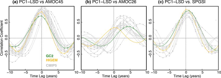
422                             P. Ortega et al.: Labrador Sea subsurface density and North Atlantic multidecadal variability

the non-regular grids. Effective resolutions over the Labrador      reducing the degrees of freedom of a series to its effective
Sea area range from 0.21◦ in the GC2 model to 1.1◦ in GISS-         value (Bretherton et al., 1999).
E2-R, GISS-E2-R-CC, and CanESM2, with these differences                Because our goal is to provide further insight into the
determining to a large extent the mean state model biases           suggested relationships established from observed trends in
and the dominant drivers (i.e. salinity or temperature) of the      the North Atlantic (e.g. Robson et al., 2016), all statistical
Labrador Sea density changes.                                       analyses in this study exploring the relationships between
   Complementing these simulations, we also consider                variables and associated lags are based on 10-year running
two control experiments with eddy-permitting resolutions.           trends. This is analogous to the calculation of a typical 10-
Specifically, we use a present-day control simulation               year running mean, but computing a linear trend instead
(i.e. with fixed radiative forcing levels from the year 1990)       over each 10-year period and keeping the slope value. Note
of the HiGEM model, with a nominal horizontal resolution            also that our main results remain similar if decadal running
in the ocean of 1/3◦ and of 0.83◦ latitude × 1.25◦ longitude        means are applied instead (not shown), as both are alternative
in the atmosphere (Shaffrey et al., 2009), and a preindus-          approaches to concentrate on the low-frequency variability.
trial control of HadGEM3-GC2 (hereafter, GC2; Ortega et             Running trends also have the particular advantage of not be-
al., 2017) with a nominal resolution in the ocean of 1/4◦           ing sensitive to long-term drifts, which are still present (and
(ORCA025) and N216 in the atmosphere (i.e. approximately            can be important for some simulations and variables) when
60 km in the mid-latitudes). The GC2 simulation is the same         running means are computed. To illustrate how decadal run-
one employed for previous analyses of Labrador Sea vari-            ning trends represent low-frequency variability and how they
ability in Robson et al. (2016) and Ortega et al. (2017). Note      compare with the decadal running means, both have been in-
that we will assume that the present-day control in HiGEM           cluded in Fig. 2b (solid thick lines vs. dashed thin lines) for
can be compared with the other preindustrial simulations due        an index of Labrador Sea density.
to the large uncertainty the latter show in their climatologi-
cal biases; so, for the sake of simplicity, we will only refer      3     Labrador Sea density as an index of multidecadal
to preindustrial control experiments from now on. Figure 1                North Atlantic variability
demonstrates that this assumption is reasonable, since the
mean Labrador Sea stratification in HiGEM is very similar           This section explores the potential of Labrador Sea density
to that in the other models.                                        as a proxy for the ocean circulation changes in the North At-
   As an observationally constrained reference, this study          lantic. As in our previous studies (Ortega et al., 2017; Robson
also includes the assimilation run from DePreSys3, a decadal        et al., 2016), the indices that we will define herein represent
prediction system from the Met Office based on GC2 (Dun-            waters within the Labrador Sea and not those that are neces-
stone et al., 2016). In the ocean, the assimilation is performed    sarily formed in the region (e.g. Labrador Sea Water). Since
through a strong nudging (10 d relaxation timescale) towards        Labrador Sea variability is affected by different processes
the full fields of a three-dimensional objective temperature        (e.g. vertical mixing, Arctic–Atlantic overflows, sea ice inter-
and salinity analysis (Smith and Murphy, 2007). Since it cov-       actions) that can be represented differently in the models in
ers a comparatively shorter period (1960–2013) and therefore        both time and space, we characterize its variability over a rel-
different timescales than the control experiments, its compar-      atively broad box (60–35◦ W, 50–65◦ N; blue box in Fig. 1a)
ison with the other simulations will be done with caution, in       that also includes part of the Irminger Sea region. Note that
particular regarding the indices of the large-scale Atlantic cir-   over this large area, EN4.2.1 shows the weakest density strat-
culation, for which other assimilation products show impor-         ification in the North Atlantic (characterized in Fig. 1a as the
tant discrepancies (Karspeck et al., 2015), thus highlighting       density difference between 1000 m and the surface).
significant uncertainty. For evaluation purposes, we also use
EN4.2.1 (Good et al., 2013), an objective analysis of monthly
                                                                    3.1    Labrador Sea density across models
temperature and salinity 3D observations developed at the
Met Office.                                                         A first indicator of potential model discrepancies is Labrador
                                                                    Sea stratification, which can lead to differences in the repre-
2.2   Methodological considerations
                                                                    sentation of deep ocean convection (i.e. weaker density strat-
                                                                    ifications will facilitate mixing, fostering convection activity,
Density values are computed from 3D salinity and poten-             and vice versa for stronger density stratifications). Figure 1b–
tial temperature fields using the International Equation of         d illustrate the intermodel differences with the vertical profile
State of Seawater (EOS-80) and are referenced to the level          of the spatially averaged Labrador Sea temperature, salinity,
of 2000 dbar (σ2 ) to give stronger emphasis to the deepwater       and density. The largest discrepancies are seen for temper-
properties.                                                         ature. Most models present their warmest waters at the sur-
   Statistical significance of correlation coefficients is as-      face, and temperatures decrease sharply to minimum values
sessed following a two-tailed Student’s t test that takes into      around 100 m and increase again at deeper levels, reaching
account the series’ autocorrelation to correct the sample size,     uniform conditions after approx 300 m. However, the loca-

Earth Syst. Dynam., 12, 419–438, 2021                                                  https://doi.org/10.5194/esd-12-419-2021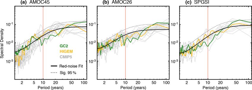
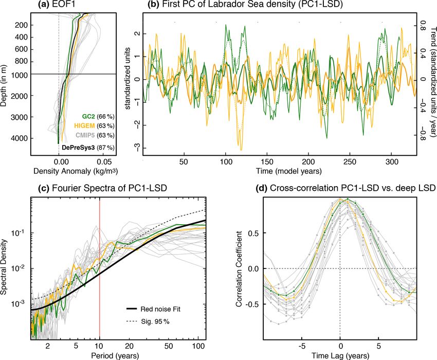
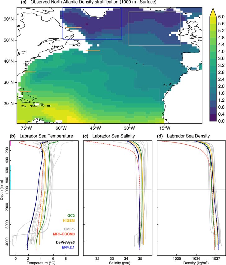
P. Ortega et al.: Labrador Sea subsurface density and North Atlantic multidecadal variability                                                423

Table 1. List of the models used for this study, their characteristics, and those of their picontrol simulations. For further details on the CMIP5
model configurations and components, please refer to Table 9A1 in Flato et al. (2013) and references therein.

  Model ID                   Long × lat ocean resolution          (number of vertical levels)    Length         Key variables available
  HadGEM3-GC2                1/4◦ × 1/4◦ (75 levels)                                             311 years      AMOC, SPGSI, LSD, NOHT
  HiGEM                      1/3◦ × 1/3◦ (40 levels)                                             341 years      AMOC, SPGSI, LSD, NOHT
  ACCESS1-0                  1◦ × 1◦ enhanced near Equator and high latitudes (50 levels)        500 years      SPGSI, LSD, NOHT
  ACCESS1-3                  1◦ × 1◦ enhanced near Equator and high latitudes (50 levels)        500 years      SPGSI, LSD, NOHT
  CCSM4                      1.125◦ × 0.27–0.64◦ (60 levels)                                     1051 years     AMOC, SPGSI, LSD
  CESM1-BGC                  1.125◦ × 0.27–0.64◦ (60 levels)                                     500 years      AMOC, LSD
  CESM1-CAM5                 1.125◦ × 0.27–0.64◦ (60 levels)                                     319 years      AMOC, LSD
  CESM1-FASTCHEM             1.125◦ × 0.27–0.64◦ (60 levels)                                     222 years      AMOC, LSD
  CESM1-WACCM                1.125◦ × 0.27–0.64◦ (60 levels)                                     200 years      AMOC, LSD
  CNRM-CM5                   0.7◦ × 0.7◦ (42 levels)                                             850 years      AMOC, SPGSI, LSD
  CanESM2                    1.4◦ × 0.93◦ (40 levels)                                            996 years      AMOC, SPGSI, LSD
  FGOALS-g2                  1◦ × 1◦ with 0.5◦ meridional in the tropical region (30 levels)     700 years      AMOC, LSD
  FGOALS-s2                  1◦ × 1◦ with 0.5◦ meridional in the tropical region (30 levels)     501 years      SPGSI, LSD, NOHT
  GFDL-ESM2G                 1◦ × 0.85◦ (63 levels)                                              500 years      SPGSI, LSD
  GISS-E2-R                  1.25◦ × 1◦ (32 levels)                                              550 years      AMOC, LSD
  GISS-E2-R-CC               1.25◦ × 1◦ (32 levels)                                              251 years      AMOC, LSD
  MPI-ESM-LR                 1.5◦ × 1.5◦ (40 levels)                                             1000 years     AMOC, SPGSI, LSD
  MPI-ESM-MR                 0.4◦ × 0.4◦ (40 levels)                                             1000 years     AMOC, SPGSI, LSD
  MPI-ESM-P                  1.5◦ × 1.5◦ (40 levels)                                             1156 years     AMOC, SPGSI, LSD
  MRI-CGCM3                  1◦ × 0.5◦ (51 levels)                                               500 years      AMOC, LSD, NOHT
  NorESM1-M                  1.125◦ × 1.125◦ (53 levels)                                         501 years      AMOC, SPGSI, LSD, NOHT
  NorESM1-ME                 1.125◦ × 1.125◦ (53 levels)                                         252 years      AMOC, SPGSI, LSD, NOHT

tion and magnitude of this temperature minimum and the two                 sity. Because of these cancelling effects, several models show
maxima are highly variable. It is important to note that the               a comparatively better representation of the subsurface den-
profile for one of the models, MRI-CGCM3, is noticeably                    sities when compared to EN4.2.1 and DePreSys3. This com-
different to the others, with a subsurface minimum more than               pensation of model shortcomings for temperature and salin-
2◦ colder than for any other model. In terms of salinity, the              ity is clearly illustrated in HiGEM, which shows remarkable
general profile is more coherent across models, with mini-                 agreement with EN4.2.1 below 500 m.
mum salinity at the surface that progressively increases with                 To represent the characteristic interannual variability of
depth and attains uniform values after 500 m. Density strati-              Labrador Sea densities (hereafter referred to as LSD for con-
fication seems to be determined by salinity, as their two verti-           sistency with previous work), we perform an empirical or-
cal profiles show similar features. This similarity includes ex-           thogonal function (EOF; Storch and Zwiers, 1999) analysis
ceptionally strong density and salinity stratification in MRI-             and extract the leading mode for the spatially averaged an-
CGCM3 compared with the other models. This stratification                  nual means of LSD (Fig. 2a), as in Ortega et al. (2017). For
is so strong that it precludes the occurrence of deep convec-              all simulations the first EOF of LSD exhibits a vertical struc-
tion (not shown). Because of this, MRI-CGCM3 is an outlier                 ture with density values that are largest at or near the surface
for many of the metrics used in the paper and has been ex-                 and gradually decrease with depth. Thus, this first EOF typ-
cluded from the subsequent analyses to facilitate the interpre-            ically reflects situations in which the density stratification,
tation of our results. We also note that the profiles for the two          as described by the climatological vertical profile in Fig. 1d,
eddy-permitting models (green and orange lines in Fig. 1b, d)              is weakened or strengthened, which happens when the cor-
lie within the spread of the CMIP5 models, indicating that                 responding principal component takes positive and negative
resolution (at least to eddy-permitting spatial scales) does               values, respectively. Some intermodel discrepancies are ev-
not drastically change stratification in the region. The De-               ident, in particular regarding the depths at which the maxi-
PreSys3 assimilation run closely matches the stratification in             mum density values are found, which can happen between
EN4.2.1, which supports the DePreSys assimilation run as a                 the surface and 500 m. Despite these differences, the domi-
reasonable observation-constrained reference for the models.               nant timescales of LSD variability seem to coincide between
The comparison of both observation-based datasets with the                 models. For example, Fig. 2b illustrates the first principal
rest of simulations suggests that, in the subsurface, all mod-             component of LSD (PC1-LSD) for GC2 and HiGEM, show-
els are too warm and most of them are too salty; these two                 ing clear multidecadal variability in both cases. Furthermore,
biases have a competing effect on the mean subsurface den-                 Fig. 2c shows the Fourier spectrum analysis of the annual

https://doi.org/10.5194/esd-12-419-2021                                                          Earth Syst. Dynam., 12, 419–438, 2021
424                           P. Ortega et al.: Labrador Sea subsurface density and North Atlantic multidecadal variability

PC1-LSD values, and most models show enhanced PC1-LSD            tral power is comparatively weaker. Important differences are
variability for periodicities between 5 and 30 years.            also seen at 50-year and longer timescales, for which the
   In addition to the PC1-LSD index we consider a deep LSD       ocean circulation indices appear to have enhanced variabil-
index as introduced in Robson et al. (2016). The deep LSD        ity with respect to PC1-LSD. Similar spectra, but with en-
index is defined as the 1000–2500 m vertical mean of the spa-    hanced variance at short timescales and reduced variance at
tially averaged density over the same region as PC1-LSD. We      the longest timescales, are obtained for the AMOC indices
now compare how both indices represent the low-frequency         when the Ekman component is kept (Supplement Fig. S1),
changes in LSD, which are described in this paper as decadal     which suggests that the low-frequency processes dominate
running trends. A lead–lag correlation between the decadal       the total AMOC variability.
trends in both PC1-LSD and deep LSD indices shows that              Figure 4a shows that decadal trends in PC1-LSD are as-
they are strongly correlated in all models. However, some        sociated with trends in the AMOC at 45◦ N (AMOC45).
differences emerge when considering the lag of maximum           Nevertheless, there is some intermodel spread regarding the
correlation (Fig. 2d). This comparison might indicate, once      lag of maximum correlation, which ranges between 0 and 2
again, that decadal variability of subsurface density is con-    years (with PC1-LSD leading), although both variables are
centrated at different depths in different models. It is also    in phase for the majority of models. The AMOC at 26◦ N
possible that both indices are sensitive to changes in deep-     (AMOC26) is also positively related to PC1-LSD, with PC1-
water formation in different locations (e.g. Irminger or GIN     LSD leading AMOC26 by 3 years on average (Fig. 4b).
seas), which could hence affect the depth and maximum lag        However, the average correlation between PC1-LSD and
of the correlations. Nevertheless, we adopt PC1-LSD for the      AMOC26 is weaker, and the spread in the magnitude and
rest of the analyses, as it has the advantage of adjusting in    lag of the maximum correlation is larger than for AMOC45.
each model to the depths at which density variability is more    Therefore, it appears that the link to the subtropics is weaker
prominent.                                                       than for 45◦ N and that AMOC coherence between subpo-
                                                                 lar latitudes and the subtropics in coupled models is model-
3.2   Labrador Sea density linkages to the ocean
                                                                 dependent. This weaker link of PC1-LSD to the subtropical
      circulation
                                                                 AMOC is not surprising, as the LSD anomalies need to prop-
                                                                 agate over a longer distance along the western boundary, al-
The link between PC1-LSD and other ocean circulation in-         lowing model differences in the representation of ocean cur-
dices in the North Atlantic is now examined. Three indices       rents and gyres to impact the timing and magnitude of the
are considered: the AMOC at two different latitudes of 26◦ N     maximum correlations. The reasons for the spread in the re-
(i.e. the same latitude as the RAPID array) and 45◦ N to cap-    lationship between PC1-LSD and AMOC26 are explored in
ture the typical variability of the subpolar AMOC and an in-     Sect. 4. A strong relationship is also found between PC1-
dex of the subpolar gyre strength. The AMOC indices are          LSD trends and those in SPGSI (Fig. 4c), which are of simi-
computed as the maximum of the North Atlantic overturn-          lar order as for AMOC45. Thus, overall, PC1-LSD is a good
ing circulation at any depth. Furthermore, the Ekman com-        proxy for the large-scale ocean circulation in the subpolar
ponent is removed to focus on the slow wind-forced and the       North Atlantic and can also be a precursor for a fraction of
thermohaline-driven (i.e. the only one that can be influenced    the AMOC variability in the subtropical Atlantic.
by the PC1-LSD directly) AMOC changes. To compute the               PC1-LSD is also a good precursor of the full AMOC
Ekman component, we vertically integrate the Ekman veloc-        variability (i.e. including the Ekman transport), although the
ities (after introducing a depth-uniform return flow to ensure   wind-induced fluctuations associated with the Ekman com-
no net meridional mass transport) following Eq. (6) in Baehr     ponent can introduce differences in the lags of the maximum
et al. (2004) with a fixed Ekman layer depth of 50 m. This       AMOC vs. PC1-LSD correlations (Supplement Fig. S2).
Ekman component is then removed at each depth level, prior       This different lag can be explained by the fact that when the
to the calculation of the AMOC indices. The subpolar gyre        Ekman component is included, the AMOC contains a sig-
strength is computed as an average of the North Atlantic         nal that is instantaneously driven by basin-scale surface wind
barotropic streamfunction in the Labrador Sea region (60–        anomalies (such as those driven by the NAO) that are, ulti-
35◦ W, 50–65◦ N), where the gyre strength is usually maxi-       mately, also linked to the heat loss in the subpolar North At-
mum. Since the SPG circulation is cyclonic and therefore as-     lantic, which induces a delayed influence on the PC1-LSD
sociated with negative barotropic streamfunction values, the     (Ortega et al., 2017). Hence, including Ekman can lead to
subpolar gyre strength index (SPGSI) is multiplied by −1 so      counterintuitive relationships in some models, in which the
that an intensification of the gyre corresponds to a positive    AMOC appears to lead the PC1-LSD changes. Also, in the
value of the index. The Fourier spectra of the raw ocean cir-    particular case of GC2, the interference of the two signals
culation indices (Fig. 3) show that, similar to the PC1-LSD,     (i.e. the subtropical Ekman and the delayed PC1-LSD) ren-
all three indices have strong multidecadal variability, with     ders the correlations in Supplement Fig. S2d insignificant,
the largest differences with respect to PC1-LSD emerging         masking out the real influence of PC1-LSD on the subtrop-
for timescales between 10 and 30 years, for which the spec-      ics. For those reasons and to ease the interpretation of the

Earth Syst. Dynam., 12, 419–438, 2021                                              https://doi.org/10.5194/esd-12-419-2021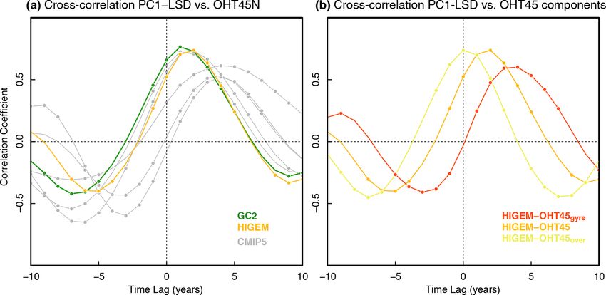
P. Ortega et al.: Labrador Sea subsurface density and North Atlantic multidecadal variability                                            425

Figure 1. (a) Climatological density (computed as σ2 at all depth levels) difference between the subsurface (1000 m) and surface in the
North Atlantic in the observational dataset EN4.2.1 (Good et al., 2013). The reference period to compute the climatology is 1960–2013.
The grey box (32–10◦ W and 47–63◦ N) encloses the region where the ESPNA-T700 index in Fig. 4d is computed. (b–d) Climatological
mean of the spatially averaged Labrador Sea (60–35◦ W, 50–65◦ N; blue box in a) temperature, salinity, and density as a function of depth
in the simulation ensemble, the DePreSys3 assimilation run, and EN4.2.1. The magenta (cyan) bars on the vertical axis correspond to the
depths that have been used to define the vertical stratification Labrador Sea indices. The horizontal orange lines by the North American coast
represent the location of the latitudinal cross sections in Figs. 10 and 11. For each model and dataset the climatology is computed for its
whole length except for EN4.2.1, which is computed for the overlap period with the DePreSys3 assimilation run.

lagged relationships, the rest of the analysis is exclusively            and those in Labrador Sea density as a function of depth,
focused on the AMOC indices without Ekman.                               with the latter leading the AMOC by up to 10 years. Fig-
   The role of PC1-LSD as a precursor of the AMOC is fur-                ure 5 reveals that the strongest link between the Labrador
ther supported by a parallel analysis in Fig. 5, looking at              Sea densities and the AMOC, both at 45 and 26◦ N, occurs
the maximum correlation between the decadal AMOC trends                  in its first 1000 m, the same levels at which the first EOF of

https://doi.org/10.5194/esd-12-419-2021                                                       Earth Syst. Dynam., 12, 419–438, 2021
426                               P. Ortega et al.: Labrador Sea subsurface density and North Atlantic multidecadal variability

Figure 2. (a) First empirical orthogonal function (EOF) as a function of depth of the spatially averaged LSD in all the preindustrial exper-
iments and in the DePreSys3 assimilation run. The percentage of variance explained by this mode in each model is included in brackets in
the legend (for the CMIP5 runs, this represents the mean value across the ensemble). Because the sign of an EOF is arbitrary, it has been
adjusted for all models (together with the sign of the respective principal component) so that both represent an increase in density stratifica-
tion. (b) Associated principal component of the spatially averaged LSD (PC1-LSD) in the two high-resolution experiments. The thin solid
lines represent the raw yearly resolved PC1-LSD time series, the thin dashed lines their respective 10-year running means, and the thick (and
slightly darker) lines their associated 10-year running trends (centred around the last year of the decade over which the trend is computed).
(c) Normalized Fourier spectra of the PC1-LSD index in each of the preindustrial simulations. The black thick line represents a red noise
process with the same first autoregressive (AR1) coefficient as PC1-LSD in GC2, and the dashed line sets the 95 % confidence interval of
this red noise process. No major differences are found when using HiGEM’s AR1 coefficient instead. The red vertical line highlights the
10-year periodicity to separate the interannual from the decadal to multidecadal timescales. (d) Lead–lag correlations between the decadal
trends in PC1-LSD and those in the deep LSD index from Robson et al. (2016), defined as the 1000–2500 m average density in the box
60–35◦ W, 50–65◦ N. Positive lags indicate that PC1-LSD leads the changes in deep LSD. Full dots denote correlation values exceeding a
95 % confidence level based on a Student’s t test that takes into account the series autocorrelation.

LSD shows the maximum loadings (Fig. 2a), which confirms                  across models. Overall, the PC1-LSD index seems to be a
the appropriateness of using PC1-LSD to represent the ocean               better choice to describe multidecadal North Atlantic vari-
circulation. The same analysis also supports a strong link                ability in multi-model comparisons, as it selects the key
between SPGSI and LSD, although in that case the largest                  depths for each model. However, PC1-LSD is mostly fo-
correlations usually happen at deeper levels (between 1000                cused on near-surface levels and therefore likely represents
and 2000 m). Note that the main conclusions drawn from                    mostly Labrador Sea forced variability. Other indices de-
PC1-LSD are also valid for the deep LSD index; however,                   scribing densities at deeper levels might be preferable to
the intermodel differences are larger in the cross-correlations           compare Labrador Sea Water of different origins across mod-
with the AMOC indices (Supplement Fig. S3). This differ-                  els and to evaluate its realism against observations.
ence could reflect the fact that the deep LSD index is more
sensitive to other influences, like the Arctic overflows (Or-
tega et al., 2017), which can be very differently represented

Earth Syst. Dynam., 12, 419–438, 2021                                                          https://doi.org/10.5194/esd-12-419-2021
P. Ortega et al.: Labrador Sea subsurface density and North Atlantic multidecadal variability 427
Figure 3. (a–c) Fourier spectra in the picontrol ensemble for the indices AMOC45, AMOC26, and SPGSI. Red noise spectra corresponding
to a first-order autoregressive process fit to GC2 indices are provided as a reference.
Figure 4. (a) Lead–lag correlations across the picontrol ensemble between the PC1-LSD index and the maximum AMOC streamfunction
at 45◦ N after the Ekman transport is removed (AMOC45). Correlations are based on 10-year running trends. Significance is assessed as in
Fig. 2d and is indicated with a circle. For positive lags, PC1-LSD leads. (b–c) The same as in (a) but between PC1-LSD and the maximum
AMOC streamfunction at 26◦ N after the Ekman transport is removed (AMOC26) and the subpolar gyre strength index (SPGSI).
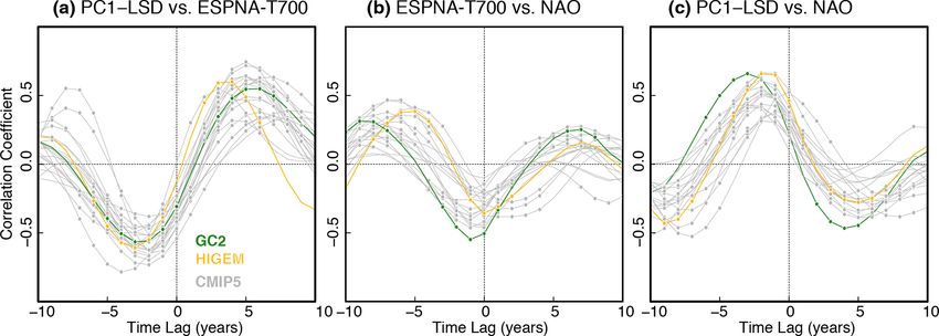
3.3 Labrador Sea density linkages to the wider North relationship is thus reminiscent of the spread found between
Atlantic PC1-LSD and AMOC26, which suggests that they might be
related. We also note significant negative correlations when
Previous studies based on the GC2 picontrol simulation have ESPNA-T700 leads PC1-LSD by 2–4 years that might be ex-
suggested LSD to also be a potential predictor of widespread plained by the opposing (and nearly concomitant) impacts
cooling events in the eastern SPNA, like the observed cooling that the NAO exerts on both variables (Fig. 6b, c). Positive
over 2005 to 2014 (Robson et al., 2016; Ortega et al., 2017). NAO phases and associated surface buoyancy forcing (Lozier
We therefore continue our exploration of the PC1-LSD index et al., 2008) lead in first instance to negative SSTs (Barrier
by investigating its link to the eastern SPNA in the multi- et al., 2014; Lohmann et al., 2009) and an almost simultane-
model ensemble. To explore this link we introduce a new ous cooling in ESPNA-T700 (Fig. 6b). In comparison, on the
index that represents the mean potential temperature in the western side of the SPNA, positive NAO phases contribute
eastern SPNA region (32–10◦ W, 47–63◦ N) averaged over to reduce vertical density stratification, favouring convection
the top 700 m of the ocean (ESPNA-T700). Lead–lag correla- and a more positive LSD index (Robson et al., 2016), which
tions between the decadal trends in PC1-LSD and this index in the models lags the NAO by 2–3 years (Fig. 6c). The fact
(Fig. 6a) show that there is a coherent relationship between that correlations between NAO and ESPNA-T700 are weaker
the two variables across models, with PC1-LSD increases than between PC1-LSD and ESPNA-T700 suggests that the
(decreases) being consistently followed by ESPNA-T700 ocean might also be playing an additional role (besides the
warmings (coolings). Nevertheless, there are intermodel dif- NAO) in controlling the ESPNA temperatures.
ferences concerning the magnitude and lag of the strongest The link between PC1-LSD and the ESPNA could be ex-
positive correlations, revealing important uncertainty in the plained through an influence of the PC1-LSD on the merid-
relationship. The spread in the PC1-LSD vs. ESPNA-T700
https://doi.org/10.5194/esd-12-419-2021 Earth Syst. Dynam., 12, 419–438, 2021428 P. Ortega et al.: Labrador Sea subsurface density and North Atlantic multidecadal variability Figure 5. (a) Maximum correlation (for any lag between 0 and 10 years) between the AMOC45 index (after the Ekman transport is removed) and Labrador Sea densities as a function of depth for all the simulations. Coloured dots indicate correlations that are significant at the 95 % confidence level. (b–c) The same as in (a) but between the AMOC26 index and LSD and between the SPGSI and LSD, respectively. Figure 6. (a) Lead–lag correlations across the picontrol ensemble between the PC1-LSD index and the vertically averaged top 700 m tem- peratures in the eastern subpolar gyre (ESPNA-T700; grey box in Fig. 1a). Correlations are based on 10-year running trends. Significance is assessed as in Fig. 2d and is indicated with a circle. For positive lags, PC1-LSD leads. (b–c) The same as in (a) but between the North Atlantic Oscillation (NAO; defined as the standardized difference in sea level pressure between the closest grid points to Azores and Reykjavik) and the ESPNA-T700 and between the NAO and the PC1-LSD, respectively. In these two cases, for negative lags the NAO leads. ional ocean heat transport. This link is now investigated in and a longer lag between OHT45 and PC1-LSD. Altogether, two eddy-permitting simulations (Fig. 7) and five CMIP5 Fig. 7a confirms that PC1-LSD is a good precursor of the models for which the ocean heat transport fields are pub- changes in the meridional ocean heat transport, although with licly available. In the two high-resolution experiments and some differences across models which might reflect a dif- two of the CMIP5 ones the decadal trends in the merid- ferent representation of certain processes. The contributions ional ocean heat transport at 45◦ N (OHT45) are strongly of two different processes to this delay are further investi- linked to those in PC1-LSD. This is a similar relationship gated in HiGEM, for which OHT was decomposed online to the one previously found in Fig. 4 between PC1-LSD at each time step into vertical and horizontal heat transports and both the AMOC45 and SPGSI, but in this case with (as in Bryan, 1969) that can be respectively interpreted as the PC1-LSD leading with a slightly longer lead time. The other “overturning” (i.e. characterized by the zonal mean transport) CMIP5 experiments support a weaker, yet significant, link and “gyre” (i.e. characterized by variations from the zonal Earth Syst. Dynam., 12, 419–438, 2021 https://doi.org/10.5194/esd-12-419-2021
P. Ortega et al.: Labrador Sea subsurface density and North Atlantic multidecadal variability 429
Figure 7. (a) Lead–lag correlations in a subset of the picontrol experiments between the PC1-LSD index and the ocean heat transport across
the 45◦ N transect (OHT45N). Note that the ocean heat content is only available for five models of the CMIP5 ensemble. Correlations are
based on 10-year running trends. (b) The same as in (a) but only in HiGEM for the different terms of the OHT45N. For positive lags,
PC1-LSD leads.
mean transport) components (Robson et al., 2018a). While cal spread have a relatively weak link between PC1-LSD and
the overturning contribution (OHT45over ) increases in phase AMOC26, although some models supporting a strong link
with the AMOC45, SPGSI, and PC1-LSD changes (Fig. 7b), are also included or remain close to the RAPID/DePreSys3
the increase in the gyre component (OHCgyre ) starts 4 years values. However, caution is recommended before defining
later. That lag could be the time required in HiGEM for the emerging constraints because models and observations are
propagation of mean and/or anomalous temperatures from not directly comparable for numerous reasons. For example,
the southern to the northern branch of the SPG. both RAPID and DePreSys3 cover shorter periods than the
simulations and relate to different background forcing con-
ditions (present day vs. preindustrial), which might imply
4 Characteristics of the intermodel spread in the
different mean states (Thornalley et al., 2018). Also, climato-
subpolar to subtropical AMOC
logical values of the AMOC26 strength are notably weaker in
DePreSys3 than in RAPID, a difference that is not explained
This section investigates which particular climatological
by the different temporal periods covered by each dataset
model features are linked to the large intermodel spread in
(not shown) and that implies that DePreSys3 might also be
the PC1-LSD vs. AMOC26 relationships. The most relevant
underestimating the real AMOC45 strength. This underesti-
model features thus identified will improve our process un-
mation could be larger than shown in Fig. 8, as evidence sug-
derstanding and can eventually be used to identify which
gests that RAPID calculations from mooring arrays might be
models are most realistic and, in turn, can deliver more re-
underestimating the AMOC strength by ∼ 1.5 Sv (Sinha et
liable projections of the future changes in the North Atlantic.
al., 2018).
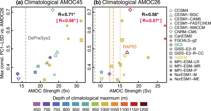
Figure 8 shows that models that simulate a stronger and
A potentially important factor behind the intermodel
deeper climatological AMOC (both at 45 and 26◦ N) tend
spread in Fig. 4b is the mean density stratification in the
to have a stronger correlation between PC1-LSD and the
Labrador Sea. Figure 9 suggests that, indeed, the PC1-LSD
subtropics. All these linear relationships between climato-
vs. AMOC26 spread is partly influenced by the density strat-
logical AMOC strength and depth as well as the PC1-LSD
ification in this region. Models that have a weaker density
vs. AMOC26 connectivity are significant at the 95 % con-
stratification (here defined as the difference between the top
fidence level. These climatological AMOC values (without
100 m and the average between 500 and 1000 m), and thus
Ekman) can be put in context with those from RAPID ob-
favour deeper convection in the Labrador Sea, generally ex-
servations and DePreSys3. RAPID observational uncertain-
hibit a stronger link between PC1-LSD and AMOC26. This
ties have been considered by including the mean values
result is robust for other stratification indices based on dif-
over three different non-overlapping periods (i.e. 2004–2007,
ferent depth levels (See Supplement Fig. S4). Differences in
2008–2012, and 2013–2016; dotted lines in Fig. 8). The scat-
density stratification across models can be due to a combina-
terplots show that the majority of models whose climatologi-
tion of different factors, from differences in the local buoy-
cal AMOC26 lies within the RAPID/DePreSys3 climatologi-
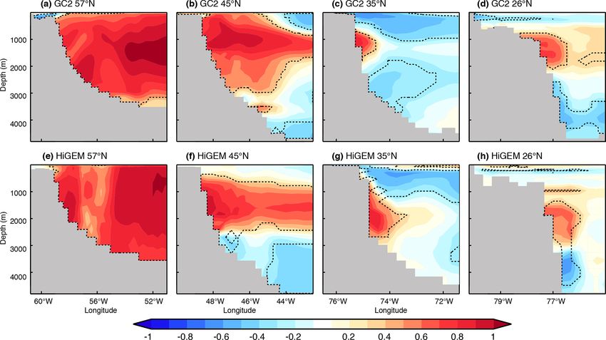
https://doi.org/10.5194/esd-12-419-2021 Earth Syst. Dynam., 12, 419–438, 2021430 P. Ortega et al.: Labrador Sea subsurface density and North Atlantic multidecadal variability Figure 8. (a, b) Scatterplot of the maximum cross-correlation value in Fig. 4b between PC1-LSD and AMOC26 against the climatologi- cal AMOC45 and AMOC26 means, respectively. All AMOC indices refer to the values after the Ekman transport signal is removed. The maximum correlations are based on 10-year running trends and always happen when PC1-LSD leads the AMOC26 index. Colours indicate the depth at which the climatological AMOC maximum occurs. The correlation coefficient between the maximum PC1-LSD correlation and the climatological mean AMOC is shown in the top left corner in black. The analogous correlation but against the depth of the mean clima- tological AMOC is shown in magenta. The presence of an asterisk indicates that the correlation is significant at the 95 % confidence level. The dashed grey vertical lines mark the climatological AMOC strength value in the DePreSys3 assimilation run. The orange vertical lines indicate the climatological value from RAPID observations (Smeed et al., 2018) from 2004 to 2016 (dashed) and in three non-overlapping sub-periods of 4 years (dotted). ancy fluxes (driven by differences in the atmospheric cir- 26◦ N. In both models, the depth of the maximum correla- culation), to differences in the representation of the Arctic tion near the continental shelf is coherent across latitudes. overflows, which are parameterized in some models (e.g. the However, in HiGEM these occur at deeper levels (1000 to CESM family; Danabasoglu et al., 2010) and explicitly re- 3000 m) compared to GC2 (1000 to 2000 m), and the differ- solved in others. No robust link between the PC1-LSD vs. ence is especially clear at 35◦ N, where the highest correla- AMOC relationship and both temperature and salinity strat- tions occur at ∼ 2000 m in HiGEM, while they are only at ification in the Labrador Sea has been found. It is also 1000 m in GC2. Similar depth differences are also found at worth mentioning that all models except CanESM2 are more 26◦ N but with slightly weaker correlations. In addition to the weakly stratified in the Labrador Sea than the observations difference in the depth of the maximum correlation between (represented herein by the DePreSys3 assimilation run and HiGEM and GC2, there are differences in the vertical struc- EN4.2.1). Hence, the real link of LSD to the AMOC26 may ture between the two models. For example, at 35◦ N in GC2, not be as strong as some models suggest. density anomalies on the western boundary form a tripole Another key aspect of the PC1-LSD vs. AMOC26 con- (low correlation above and below the maximum correlation nectivity is the western boundary density (WBD). Indeed, at ∼ 1000 m), but in HiGEM the density anomalies form a boundary density is critical to the mechanism through which dipole (Fig. 10g). We note some differences in bathymetry LSD influences the AMOC at lower latitudes. Positive (neg- at this latitude (which is steeper in HiGEM), which might ative) LSD anomalies propagate equatorward following this partly explain some of the differences in terms of the density boundary, and as they do so they strengthen (weaken) the correlation structure. zonal density gradient, triggering a thermal wind response Figure 11 shows that the diversity in the depth of these that accelerates (decelerates) the AMOC. In the following boundary densities is even more evident when including the we investigate differences in the propagation of boundary CMIP5 models. The depth of the maximum correlation be- densities across models and if these differences can affect tween PC1-LSD and the western boundary density at the four the intermodel PC1-LSD vs. AMOC26 spread. Figure 10 fo- latitudinal sections relates linearly (and significantly at the cuses on the two high-resolution simulations, wherein impor- 95 % confidence level) across models to their PC1-LSD vs. tant differences already manifest. It represents the in-phase AMOC26 correlation. In this case, models exhibiting maxi- correlations of PC1-LSD with the density fields (defined as mum correlations with the WBDs at deeper levels generally σ2 ) near the western boundary at four different longitudinal show stronger links between PC1-LSD and the subtropical transects: 57 (cutting across the Labrador Sea), 45, 35, and AMOC. In DePreSys, our observationally constrained refer- Earth Syst. Dynam., 12, 419–438, 2021 https://doi.org/10.5194/esd-12-419-2021
P. Ortega et al.: Labrador Sea subsurface density and North Atlantic multidecadal variability 431
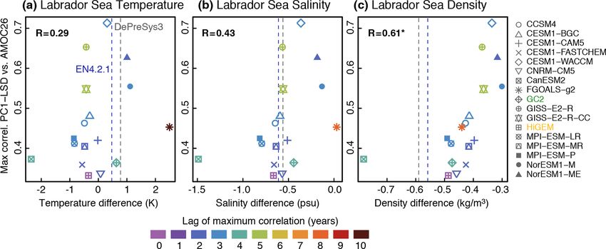
Figure 9. (a) Scatterplot of the maximum cross-correlation value in Fig. 4b between PC1-LSD and AMOC26 (without the Ekman com-
ponent) against the climatological mean of the Labrador Sea temperature stratification index (computed as the difference of the vertical
means in the levels 0–100 m minus the vertical means in the levels 500–1000 m; see Fig. 1). The maximum correlations are based on 10-year
running trends. The correlation coefficient between the two metrics is shown in the top left corner. The presence of an asterisk indicates that
the correlation is significant at the 95 % confidence level. Colours indicate the lag at which the maximum correlation between PC1-LSD and
AMOC26 is obtained. The grey (blue) vertical lines depict the mean stratification value in the DePreSys3 assimilation run (EN4.2.1). In both
cases, their overlap period is used to compute the climatology (i.e. 1960–2013). (b–c) The same as in (a) but for the Labrador Sea salinity
and density (defined as σ2 ), respectively.
ence (dashed grey lines in Fig. 11), these maximum corre- – All the simulations show clear multidecadal variability
lations tend to occur at relatively shallow levels when com- in Labrador Sea density. There is also a close link be-
pared with the multi-model ensemble. We have also checked tween LSD and the strength of the subpolar Atlantic
if models with stronger correlations with the WBDs (as rep- Ocean circulation, with positive density anomalies lead-
resented by the PC1-LSD and WBD maximum correlations ing to a strengthening of the Atlantic Meridional Over-
at every latitudinal section) also support a stronger link be- turning Circulation (AMOC) at 45◦ N and the subpolar
tween the PC1-LSD and the AMOC, but this linearity as- gyre (SPG) circulation.
sumption only holds true at 57◦ N (correlations in magenta
in Fig. 11). This suggests that the depth along which WBDs – The relationship between anomalous LSD and the
propagate southward and/or the vertical structure of anoma- strength of the AMOC at 26◦ N – the latitude of the
lies are the key aspects to understand and potentially narrow RAPID array measurements – is also positive in the
down the spread. simulations, but there are significant intermodel differ-
ences in both the strength of the relationship and the lag
of maximum correlation. This uncertainty implies that
the connectivity of LSD to the subtropics and latitudi-
5 Conclusions and discussion
nal AMOC coherence is model-dependent.
This article has explored, in a multi-model context, the link- – The connectivity between anomalies in LSD and the
ages between subsurface density in the subpolar North At- AMOC at 26◦ N is sensitive to different model fea-
lantic (SPNA) and the ocean circulation further south. In tures, including the strength and depth of the climato-
particular, it has explored the role of Labrador Sea den- logical AMOC maximum, the mean density stratifica-
sity (LSD) in driving western boundary density anomalies tion in the Labrador Sea, and the depths at which the
(WBD) and the ocean circulation, as well as the impact on LSD propagates southward along the western bound-
upper-ocean temperature changes in the SPNA. The analysis ary. Stronger LSD connectivity to the subtropics tends
was based on two control simulations with eddy-permitting to occur in models with a stronger and deeper AMOC,
models (a preindustrial one with HadGEM3-GC2 and a weaker Labrador Sea stratification, and western bound-
present-day one with HiGEM) and on 20 CMIP5 preindus- ary density propagating at deeper levels.
trial experiments. Furthermore, where possible these charac-
teristic model features have been computed in observational – Observationally derived constraints of the model-based
datasets and in a simulation assimilating observations. The relationships tend to suggest that the link between LSD
major findings are listed below. and the subtropical AMOC is weak. This suggests that
https://doi.org/10.5194/esd-12-419-2021 Earth Syst. Dynam., 12, 419–438, 2021You can also read