Spatio-temporal controls of C-N-P dynamics across headwater catchments of a temperate agricultural region from public data analysis - HESS
←
→
Page content transcription
If your browser does not render page correctly, please read the page content below
Hydrol. Earth Syst. Sci., 25, 2491–2511, 2021
https://doi.org/10.5194/hess-25-2491-2021
© Author(s) 2021. This work is distributed under
the Creative Commons Attribution 4.0 License.

Spatio-temporal controls of C–N–P dynamics across headwater
catchments of a temperate agricultural region from public
data analysis
Stella Guillemot1,2 , Ophelie Fovet1 , Chantal Gascuel-Odoux1 , Gérard Gruau3 , Antoine Casquin1 , Florence Curie2 ,
Camille Minaudo4 , Laurent Strohmenger1 , and Florentina Moatar5,2
1 UMR  SAS, INRAE, Institut Agro, 35000 Rennes, France
2 Université
           de Tours, EA 6293 GéHCO, 37200 Tours, France
3 OSUR, Geosciences Rennes, CNRS, Université Rennes 1, 35000 Rennes, France
4 EPFL, Physics of Aquatic Systems Laboratory, 1015 Lausanne, Switzerland
5 INRAE, RIVERLY, 69625 Villeurbanne, France

Correspondence: Ophelie Fovet (ophelie.fovet@inrae.fr)

Received: 26 May 2020 – Discussion started: 22 June 2020
Revised: 14 March 2021 – Accepted: 23 March 2021 – Published: 18 May 2021

Abstract. Characterizing and understanding spatial variabil-      according to their seasonal cycles. In addition, the quality of
ity in water quality for a variety of chemical elements is        annual maximum NO3 concentration was in phase with max-
an issue for present and future water resource management.        imum flow when the base flow index was low, but this syn-
However, most studies of spatial variability in water qual-       chrony disappeared when flow flashiness was lower. These
ity focus on a single element and rarely consider headwater       DOC–NO3 seasonal cycle types were related to the mixing
catchments. Moreover, they assess few catchments and focus        of flow paths combined with the spatial variability of their
on annual means without considering seasonal variations. To       respective sources and to local biogeochemical processes.
overcome these limitations, we studied spatial variability and    The annual maximum SRP concentration occurred during the
seasonal variation in dissolved C, N, and P concentrations at     low-flow period in nearly all catchments. This likely resulted
the scale of an intensively farmed region of France (Brittany).   from the dominance of P point sources. The approach shows
We analysed 185 headwater catchments (from 5–179 km2 )            that despite the relatively low frequency of public water qual-
for which 10-year time series of monthly concentrations and       ity data, such databases can provide consistent pictures of the
daily stream flow were available from public databases. We        spatio-temporal variability of water quality and of its drivers
calculated interannual loads, concentration percentiles, and      as soon as they contain a large number of catchments to com-
seasonal metrics for each element to assess their spatial pat-    pare and a sufficient length of concentration time series.
terns and correlations. We then performed rank correlation
analyses between water quality, human pressures, and soil
and climate features. Results show that nitrate (NO3 ) con-
centrations increased with increasing agricultural pressures      1   Introduction
and base flow contribution; dissolved organic carbon (DOC)
concentrations decreased with increasing rainfall, base flow      As a condition for human health, food production, and
contribution, and topography; and soluble reactive phospho-       ecosystem functions, water quality is recognized as “one of
rus (SRP) concentrations showed weaker positive correla-          the main challenges of the 21st century” (FAO and WWC,
tions with diffuse and point sources, rainfall and topography.    2015; UNESCO, 2015), and potential impacts of climate
An opposite pattern was found between DOC and NO3 : spa-          change on water quality are even more challenging (White-
tially, between their median concentrations, and temporally,      head et al., 2009). To better estimate and reduce human im-
                                                                  pact on water quality, water scientists are expected to pro-

Published by Copernicus Publications on behalf of the European Geosciences Union.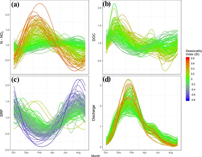
2492                                                        S. Guillemot et al.: Spatio-temporal controls of C–N–P dynamics

vide integrated understanding of multiple pollutants (Cos-         istics on water concentrations or loads varied by season be-
grove and Loucks, 2015). Eutrophication risks (Dodds and           cause nutrient sources and biological and physico-chemical
Smith, 2016) are considered the main factors that decrease         processes that influence nutrient mobilization and transfer in
the quality of surface water, according to objectives set by       catchments (e.g. vegetation uptake, in-stream biomass pro-
the European Union Water Framework Directive. Mitigating           duction, denitrification) changed with the hydrological, light,
the problem of eutrophication involves considering at least        and temperature conditions (Ågren et al., 2007; Fasching et
the three major elements: carbon (C), nitrogen (N), and phos-      al., 2016; Gardner and McGlynn, 2009). Some variability
phorus (P) (Le Moal et al., 2019).                                 in seasonal patterns of dissolved C, N, and/or P concentra-
   In addition, the quality of headwater catchments has been       tions among headwater catchments has been reported (e.g.
studied less than large rivers (Bishop et al., 2008), despite      Van Meter et al., 2019; Abbott et al., 2018b; Duncan et al.,
their influence on downstream water quality (Alexander et          2015; Martin et al., 2004). Identifying these patterns is rel-
al., 2007; Barnes and Raymond, 2010; Bol et al., 2018) and         evant from a management viewpoint as they may indicate
higher spatial variability in their concentrations (Abbott et      changes in the locations of C, N, or P sources or their trans-
al., 2018a; Temnerud and Bishop, 2005). One reason for this        fer pathways.
is that most water quality monitoring networks coincide with          Thus, to date, analysis of spatial variability in water quality
the location of drinking-water production facilities, which        at the headwater scale
explains why they focus on large rivers. Nonetheless, investi-
gating spatial variability in upstream water quality is relevant     1. is usually restricted to one element, although multi-
for understanding what causes it to degrade, targeting loca-            element approaches are becoming more frequent (Ed-
tions with the greatest disturbances, and identifying which             wards et al., 2000; Heppell et al., 2017; Lintern et al.,
remediation policies would be most cost-effective.                      2018; Mengistu et al., 2014; Mutema et al., 2015).
   In non-agricultural headwater catchments, spatial variabil-
                                                                     2. is particularly rare for headwater catchments with sim-
ity in dissolved organic C (DOC) concentrations in streams
                                                                        ilar human pressures (e.g. intensive farming), despite
has been related to topography, wetland coverage, and soil
                                                                        the high variability in water quality sometimes observed
properties such as clay content or pH (Andersson and Ny-
                                                                        among them (e.g. Thomas et al., 2014).
berg, 2008; Brooks et al., 1999; Creed et al., 2008; Hytte-
born et al., 2015; Musolff et al., 2018; Temnerud and Bishop,        3. often uses mean annual values (concentration or load)
2005; Zarnetske et al., 2018). Stream DOC concentrations                to describe spatial variability in water quality among
and composition in agricultural and urbanized areas also gen-           catchments, with little or no analysis of seasonal pat-
erally differ greatly from those in semi-natural or pristine            terns despite their frequent occurrence (Van Meter et al.,
catchments (Graeber et al., 2012; Gücker et al., 2016). Over            2019; Abbott et al., 2018b; Liu et al., 2014; Halliday et
large gradients of human impact (e.g. from undisturbed to               al., 2012; Mullholland and Hill, 1997).
urban catchments), the cover of agricultural and urban land
uses often appears as a key factor that explains differences         4. is usually restricted to a few catchments: multiple-
in stream chemistry of C, N, and P species (e.g. Barnes and             catchment studies on multiple elements are uncommon,
Raymond, 2010; Edwards et al., 2000; Mutema et al., 2015)               despite their ability to identify dominant controlling fac-
and even silica (Onderka et al., 2012). Conversely, in mostly           tors better.
undisturbed catchments (Mengistu et al., 2014) or in rural
                                                                     We studied the spatial variability and seasonal variation
catchments where human pressure are low (Heppell et al.,
                                                                   in water quality of 185 headwater catchments (from 5–
2017; Lintern et al., 2018), “natural” controls such as to-
                                                                   179 km2 ) draining Brittany, an intensively farmed region of
pography, geology, and flow paths are more frequently high-
                                                                   France. Our analysis focuses on dissolved C, N, and P con-
lighted as the main factors that explain spatial variability in
                                                                   centrations as DOC, nitrate (NO3 ), and soluble reactive P
C, N, and P.
                                                                   (SRP), respectively. We hypothesized the following:
   Besides being spatially variable, C, N, and P concen-
trations also vary temporally. The variability of concentra-         1. Human (i.e. rural and urban) pressures determine spa-
tions with flow has been described in several studies using             tial variability in NO3 and SRP concentrations (Preston
concentration–flow relationships at event (Fasching et al.,             et al., 2011; Melland et al., 2012; Dupas et al., 2015a;
2019) or inter-annual to long-term scales (Basu et al., 2010,           Kaushal et al., 2018), while soil and climate character-
2011; Moatar et al., 2017). Concentrations also vary season-            istics, including light and temperature along the stream,
ally in streams and rivers (Aubert et al., 2013; Dawson et al.,         determine that in DOC and possibly SRP (Lambert et
2008; Duncan et al., 2015; Exner-Kittridge et al., 2016; Lam-           al., 2013; Humbert et al., 2015; Gu et al., 2017).
bert et al., 2013), as does the composition of dissolved or-
ganic matter (Griffiths et al., 2011; Gücker et al., 2016). This     2. Seasonal variations in water quality provide informa-
seasonality can also be spatially structured. Several studies           tion about spatial variability in biogeochemical sources
showed that the relative importance of catchment character-             and/or reactivity in catchments as a function of changes

Hydrol. Earth Syst. Sci., 25, 2491–2511, 2021                                       https://doi.org/10.5194/hess-25-2491-2021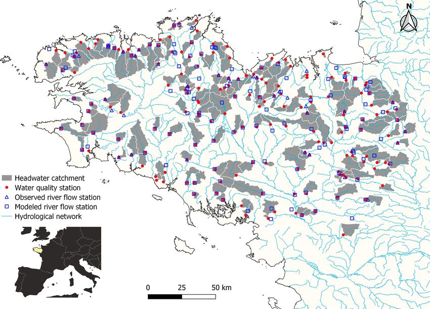
S. Guillemot et al.: Spatio-temporal controls of C–N–P dynamics                                                              2493

       in water pathways and are correlated in part with spatial   ing to the following two criteria: (i) independence, with no
       variability in concentrations and loads.                    overlap of the drained areas of the water-quality stations se-
                                                                   lected, and (ii) availability of at least 80 measurements of
   We selected headwater catchments for which relevant time        DOC, NO3 , and SRP concentrations at the same station (af-
series of DOC, NO3 , and SRP concentrations and stream             ter removing outliers based on expert knowledge, i.e. val-
flow were available (10 years of consecutive data measured         ues > 200 mg N L−1 or 5 g P L−1 ) over 10 calendar years
at least monthly). In addition to estimating interannual loads,    (2007–2016). We selected 185 stations (83 % and 17 % from
we calculated concentration metrics for each element to as-        OSUR and HYDRE/BEA, respectively) (hereafter, “concen-
sess the spatial variability and temporal variation in water       tration (C) stations”), which had mean frequencies of 12, 14,
quality. Generalized additive models (GAMs) were applied           and 11 analyses per year for DOC, NO3 , and SRP, respec-
to the time series to highlight average patterns of seasonal       tively. We checked that there was no bias in the timing of con-
variation. Correlations between the water quality metrics and      centration data: OSUR database has fixed and regular sam-
the geological, soil, climatic, hydrological, land cover, and      pling frequencies while we noticed a few time series where
human pressure characteristics of the corresponding headwa-        summer periods were less sampled in the HYDRE/BEA data
ter catchments were evaluated using rank correlation analy-        for some years only.
ses.                                                                  Each C station was paired with a hydrometric station (Q).
                                                                   Observed daily streamflow data from the national hydro-
                                                                   metric network (http://www.hydro.eaufrance.fr/, last access:
2     Materials and methods                                        28 April 2021) were used when draining headwater catch-
                                                                   ments for C and Q stations shared at least 80 % of their areas
2.1    Study area
                                                                   (25 % of cases). When observed Q data were not available,
Brittany is a 27 208 km2 region in western France. Its             or at a frequency less than 320 measurements per year from
bedrock is composed mainly of a crystalline substratum             2007–2016 (75 % of cases), discharge data were simulated
dominated by granite and schist (Supplement Fig. S1b).             using the GR4J model (Perrin et al., 2003). The headwater
Its topography is moderate, with elevation ranging from 0–         catchments selected and their associated C and Q stations
330 m a.s.l. Its climate is temperate oceanic, with precipita-     were distributed throughout Brittany (Fig. 1).
tion ranging from 531 mm yr−1 in the east to 1070 mm yr−1             The 185 headwater catchments selected cover ca. 32 % of
on the western coasts (regional median of 723.0 mm yr−1 )          Brittany’s area. Despite having a similar hydrographic con-
(Fig. S1a), with a mean annual temperature of 12 ◦ C. The re-      text dominated by subsurface flow, the catchments have large
gional hydrographic network is dense, with a mean density of       differences in topography, geology, hydrology, and diffuse
1 km km−2 . Overall, 56.6 % of the region was utilized agri-       and point-source pressures of N and P. We used a set of catch-
cultural area (UAA) in 2017 (data from DREAL Bretagne,             ment descriptors to quantify this variability (Table 1) (see
Brittany’s Agency for Environment, Infrastructure, and             Fig. S2 for their statistical distribution and S3 for their cor-
Housing), which represented 6 % of national UAA in 2016.           relations). The descriptors selected included a set of spatial
Of total French production, Brittany produces 17.4 % of milk       metrics for element sources (e.g. land use, pressure, soil con-
and dairy products, 20 % of pork products, and 17 % of             tents) and for mobilization and retention processes (e.g. hy-
eggs and poultry (Chambres d’agriculture de Bretagne, 2016         drology, climate, topography, geology, and soil properties).
data). At the canton (administrative district) scale, mean N          The headwater catchments range in area from 5–179 km2
and P surpluses are high and have high spatial variability         (median of 38 km2 ), and the density of each one’s hydro-
(standard deviation (SD)): 50.01 ± 26.59 kg N ha−1 yr−1 and        graphic network ranges from 0.47–1.49 km km−2 (median
22.52 ± 12.66 kg P ha−1 yr−1 (Fig. S1e, f). The region has a       of 0.90 km km−2 ). Strahler stream order is 3 for 36 % of
population of ca. 3.3 million inhabitants (data 2017), some        the catchments, 2 for 18 %, 4 for 17 %, and 1 for 11 %.
scattered throughout the region, and some concentrated in a        Substrate composition is dominated by schists/mica schists
few cities and near the coasts (Fig. S1c, d).                      (44 %) or granites/gneisses (31 %). In the topsoil horizon
                                                                   (0–30 cm), the soil organic C content varies greatly from
2.2    Stream data selection and headwater                         18.6–565.4 g kg−1 (median of 126.9 g kg−1 ), while the to-
       characteristics                                             tal P (Dyer method) content varies from 0.6–1.4 g kg−1 (me-
                                                                   dian of 0.9 g kg−1 ). Land use is largely agricultural, although
Water quality data consisted of time series of DOC, NO3 ,          some catchments have high percentages of forested and ur-
and SRP concentrations, extracted from two public moni-            banized areas. Riparian wetlands cover 12.3 %–36.3 % of
toring networks – OSUR (Loire-Brittany Water Agency, 554           catchment area (median of 22.4 %), forest covers 1.3 %–
sites) and HYDRE/BEA (DREAL Bretagne, ca. 1964 sites),             55.7 % (median of 13.2 %), pasture covers 10.3 %–46.7 %
measured for regulatory monitoring, regional contracts, or         (median of 25.6 %), summer crops cover 6.5 %–50.3 % (me-
specific programmes. Concentrations were measured from             dian of 27.8 %), and winter crops cover 7.0 %–51.0 % (me-
grab samples. Headwater catchments were selected accord-           dian of 22.7 %). The N and P surplus (potential diffuse

https://doi.org/10.5194/hess-25-2491-2021                                       Hydrol. Earth Syst. Sci., 25, 2491–2511, 2021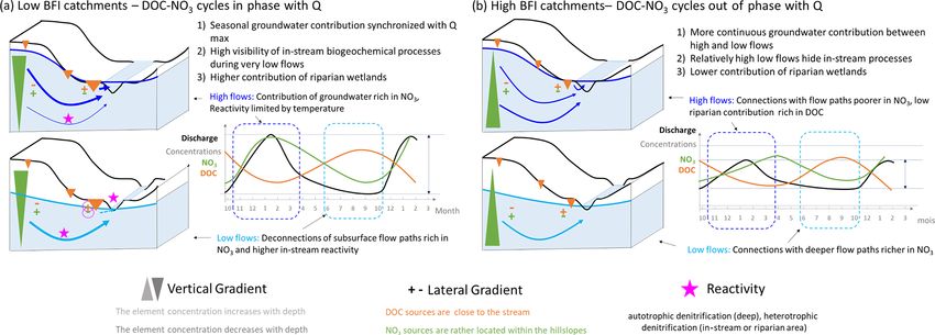
2494                                                         S. Guillemot et al.: Spatio-temporal controls of C–N–P dynamics

Figure 1. Locations of the 185 study headwater catchments where dissolved organic carbon, nitrate, and soluble reactive phosphorus con-
centrations were monitored monthly at the outlet from 2007–2016, and paired discharge stations where daily records of stream flow were
available from observations or modelling.

agricultural sources) varies from 12.9–96.0 kg N ha−1 yr−1            a 10-year period (2007–2016), with 8–12 C–Q values per
(median of 47.7) and 2.8–63.2 kg P ha−1 yr−1 (median of               year. However, a 5-year period (2010–2014) was considered
18.9), respectively. Urban areas cover 1.3 %–31.8 % of the            to analyse the spatial variability because it minimized data
headwater catchments (median of 6 %), with point-source               gaps (in C and Q time series) among all stations simultane-
input estimates ranging from 0–6.2 kg N ha−1 yr−1 and 0–              ously.
0.626 kg P ha−1 yr−1 . These data illustrate relative diver-             To calculate interannual DOC, NO3 , and SRP loads for
sity in human pressures among the catchments despite a                each headwater catchment, we tested different methods and
regional context of intensive agriculture. The daily mean             selected the most suitable, depending on the reactivity of the
flow (Qmean) varies from 4.8–24.5 L s−1 km−2 (median                  element with flow. When C–Q relationships were relatively
of 10.8 L s−1 km−2 ), the median of annual minimum of                 flat or diluted (NO3 ) or slowly mobilized (DOC) during high
monthly flows (QMNA) varies from 0.2–5.9 L s−1 km−2 , and             flow (Q > Q50), we used the discharge-weighted concen-
the flow flashiness index (W 2), defined as the percentage of         tration (DWC) method (Eq. 1), which estimates loads with
total discharge that occurs during the highest 2 % of flows           lower uncertainties (Moatar and Meybeck, 2007; Raymond
(Moatar et al., 2020), ranges from 10 %–28 %.                         et al., 2013):
                                                                                      Pn
                                                                                 k          Ci Qi
2.3     Data analysis                                                 DWC = × Pi=1       n        Q,                             (1)
                                                                                 A       i=1 Qi

2.3.1    Concentration and load metrics                               where DWC is the mean of annual loads (kg yr−1 ha−1 ), Ci
                                                                      is the instantaneous concentration (mg L−1 ), Qi is the corre-
To analyse spatial variability in DOC, NO3 , and SRP con-             sponding flow rate (m3 s−1 ), Q is the mean annual flow rate
centrations in streams, we calculated their 10th, 50th, and           calculated from daily data (m3 s−1 ), A is the area of the head-
90th percentiles of concentration (C10, C50, and C90, re-             water catchment (ha), k is a conversion factor (31 536), and
spectively) for each headwater catchment from 2007–2016.              n is the number of C–Q pairs per year.
We also calculated the ratio of the coefficient of variation             The loads estimated by the DWC method were corrected
(CV) of mean concentration (CVcmean ) and to that of mean             for bias (Moatar et al., 2013). Precisions were calculated
flow (CVqmean ) to compare spatial variabilities in concen-           from the number of samples (n), number of years, export
trations and stream flow. We estimated interannual loads for          regime exponent (b50high ), and W 2 (Moatar et al., 2020).

Hydrol. Earth Syst. Sci., 25, 2491–2511, 2021                                          https://doi.org/10.5194/hess-25-2491-2021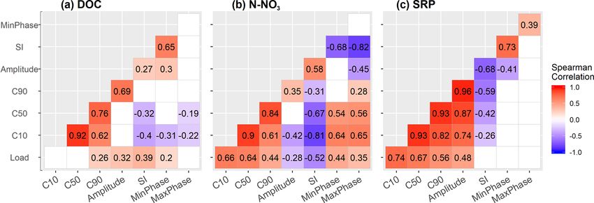
S. Guillemot et al.: Spatio-temporal controls of C–N–P dynamics                                                                2495

   To calculate SRP loads, regression methods were more             15 March) concentrations of an element, as follows (Eq. 4):
suitable (because of strong concentration patterns when
stream flow increases). We averaged the loads estimated by                  Cwinter − Csummer
                                                                    SI =                      ,                                  (4)
two regression methods developed by Raymond et al. (2013)                   Cwinter + Csummer
− integral regression curve (IRC) and segmented regression
curve (SRC) – both based on a regression between concen-            where Cwinter and Csummer are the averages of winter and
tration and flow:                                                   summer concentrations, calculated from daily values from
                                                                    fitted GAM. Positive values of SI (near 1) indicate that
                                                                    Cwinter > Csummer , while negative values (near −1) indicate
     k 0 Xn                                                         that Cwinter < Csummer . We considered that SI values close to
IRC =   ×    CQ
          i=1 i i
                                                             (2)
     A                                                              0 (from −0.1 to 0.1) indicated that Cwinter equaled Csummer .
     k 0 Xm1              Xm2
                                                                    The SI integrates both amplitude and phasing features of the
SRC = ×     i=1
                Cinfi Qi +  i=1
                                C supi Q i   ,               (3)
      A                                                             seasonal signal. These five metrics, obtained from daily sim-
                                                                    ulations of the GAMs, are linked to geographical variables
where IRC and SRC are the mean of annual loads                      (Sect. 2.2), even if particular solutes in some catchments do
(kg yr−1 ha−1 ); Ci , Csupi , and Cinfi are instantaneous concen-   not present any seasonality.
trations estimated by the regression curves (mg L−1 ); Csupi
and Cinfi are concentrations estimated for flows above and          2.3.3    Statistical analyses
below the median flow, respectively; n = 365 d; m1 and m2
are numbers of days with daily flows below and above the            To compare the concentration metrics of the elements, a mul-
median flow, respectively; k 0 is a conversion factor (86.4);       tivariate analytical approach, principal component analysis
and A is the area of the headwater catchment (ha).                  (PCA), was performed for the nine variables of concentration
                                                                    percentiles (C10, C50, and C90) of DOC, NO3 , and SRP for
                                                                    the dataset of 185 headwater catchments. PCA was chosen
2.3.2   Seasonal signal
                                                                    despite its assumption of linear relationships between vari-
                                                                    ables, because it provides a graphical representation of cor-
Seasonal dynamics of discharge and solute concentrations            relations between variables or groups of variables and their
were modelled using GAMs (Wood, 2017), which can es-                contributions to the variance. To identify dominant drivers
timate smoothed seasonal dynamics from time series (Mu-             of spatial variability in concentration percentiles, seasonality,
solff et al., 2017). The smoothing function was a cyclic cu-        and loads of DOC, NO3 , and SRP, we calculated Spearman’s
bic spline fitted to the month of the year (1–12); thus, the        rank correlation (rs ) between these water-quality metrics and
ends of the spline were forced to be equal, using the R pack-       the descriptors of the headwater catchments (Table 1). We
age mgcv. We did not consider a long-term trend in the time         considered a rank correlation to be significant if the corre-
series over the 10 years, for two reasons. First, significant       sponding p value was ≤ 0.05. All analyses were performed
long-term trends (according to Mann–Kendall tests) had low          using R software (v. 3.6.1) with packages mgcv, hydroGOF,
slopes: mean Theil–Sen slopes ranged from −3 % to 0 % of            hydrostats, FactoMineR, tidyverse, lubridate, reshape2, plyr,
the median concentration (while mean seasonal relative am-          ggcorrplot, and ggplot2 (Grolemund and Wickham, 2011; Le
plitudes exceeded 50 %). Second, performance of the GAMs            et al., 2008; Wickham, 2011, 2016; Wood, 2017; Zambrano-
did not increase significantly when a long-term trend was           Bigiarini, 2020).
added: the mean-adjusted coefficient of determination (Rsq)
increased from 0.16 to 0.18 for DOC and from 0.30 to 0.40
for NO3 . We considered a seasonal dynamic to exist when            3     Results
the GAM-adjusted coefficient of determination was greater
than 0.10.                                                          3.1     Spatial variability in concentrations and loads
   Seasonal dynamics of the concentrations of the three so-
lutes (DOC, NO3 , and SRP) and river discharge were then            The C50 of the 185 headwater catchments ranged from
analysed using five metrics calculated from the daily simula-       2–14.6 mg C L−1 for DOC, 0.9–15.8 mg N L−1 for NO3 ,
tions of the GAMs. The first three were the annual amplitude        and 8–241 µg P L−1 for SRP (with 75 % of the SRP
(Ampli; i.e. annual maximum minus annual minimum), and              C50 < 64 µg P L−1 ). The C50 displayed spatial gradients:
the mean time in which annual maximum and minimum con-              rivers with DOC concentrations > 5 mg C L−1 were located
centrations occurred (MaxPhase and MinPhase, respectively;          in eastern Brittany, while the highest NO3 concentrations
in months from 1 January). The next was Ampli standard-             were located on the west coast (Fig. 2). In contrast, the high-
ized by the corresponding mean concentration to compare the         est concentrations of SRP (C50 > 68 µg P L−1 ) were located
three solutes. The last metric was a seasonality index (SI),        in northern Brittany.
which measures the relative importance of summer (1 June               The two first axes of the PCA (Fig. 3a) performed on the
to 31 July) concentrations compared to winter (15 January to        percentiles of DOC, NO3 , and SRP concentrations of the 185

https://doi.org/10.5194/hess-25-2491-2021                                           Hydrol. Earth Syst. Sci., 25, 2491–2511, 2021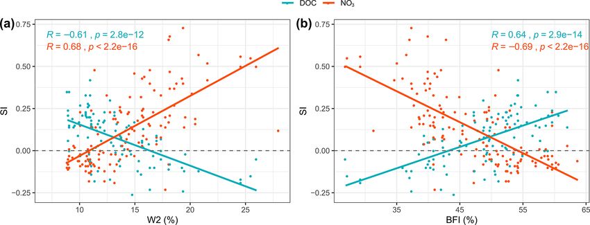
2496                                                           S. Guillemot et al.: Spatio-temporal controls of C–N–P dynamics

Table 1. Headwater catchment descriptors identified as potential explanatory variables of spatial variability and temporal variation in dis-
solved organic carbon (DOC), nitrate (NO3 ), and soluble reactive phosphorus (SRP) in stream and river water. meanTWI = log tanα β , where
α is the drainage area (ha) and β is the downstream slope (%) (Merot et al., 2003).

          Type               Descriptor name     Unit         Definition                         Source
          Topography         Area                km2          Drainage area of the monitoring    Web processing service “Ser-
                                                              station                            vice de Traitement de Modèles
                                                                                                 Numériques de Terrain” and
                                                                                                 DEM 50 m by IGN
                             Elevation           m            Mean elevation of headwater        DEM 25 m by IGN
                                                              catchment
                             Density_hn          km km−2      Density of the hydrographic        BD Carthage by IGN
                                                              network
                             meanTWI             cf. legend   Average topographic wetness        DEM 25 m by IGN
                                                              index of the headwater catch-
                                                              ment
                             IDPR                –            Hydrographic network devel-        http://infoterre.brgm.fr/ (last
                                                              opment and persistence index       access: 28 April 2021) BRGM
                                                                                                 data and geoservices portal
                                                                                                 (Mardhel and Gravier, 2004)
          Geology            Granite_pm          %            Percentage of granite and          Web mapping service “Carte
                                                              gneiss area                        des Sols de Bretagne” by
                                                                                                 UMR 1069 SAS INRAE –
                                                                                                 Agrocampus Ouest http://www.
                                                                                                 sols-de-bretagne.fr/ (last ac-
                                                                                                 cess: 28 April 2021)
                             Schist_pm           %            Percentage of schist and mica
                                                              schist area
                             Other_pm            %            Percentage of various geologi-
                                                              cal substrata
          Soil               Erosion             %            Percentage of area with high to    Erosion risk map estimated
                                                              very high erosion risk (derived    from MESALES by GIS
                                                              from land use, topography, and     Sol, INRAE from Colmar et
                                                              soil properties)                   al. (2010)
                             OC_soil             g kg−1       Organic carbon content in the      Web mapping service from
                                                              topsoil horizon (0–30 cm)          BDAT database, Saby et
                                                                                                 al. (2015) by GIS Sol
                             Thick_soil          cm           Classes of dominant soil           Web mapping service “Carte
                                                              thicknessa                         des Sols de Bretagne” by UMR
                                                                                                 1069 SAS INRAE – Agrocam-
                                                                                                 pus Ouest
                             TP_soil             g kg−1       Total phosphorus content in the    Web mapping service from
                                                              topsoil horizon (0–30 cm)          BDAT database by GIS Sol
          Land use           SummerCrop          %            Percentage of summer cropb         OSO         database,      CES-
                                                              land                               BIO,        land-cover      map
                                                                                                 2016      (1 ha)   from     http:
                                                                                                 //osr-cesbio.ups-tlse.fr/~oso/
                                                                                                 (last access: 28 April 2021)
                             WinterCrop          %            Percentage of winter cropc land
                             Forest              %            Percentage of forest land

Hydrol. Earth Syst. Sci., 25, 2491–2511, 2021                                             https://doi.org/10.5194/hess-25-2491-2021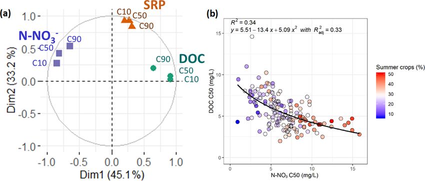
S. Guillemot et al.: Spatio-temporal controls of C–N–P dynamics                                                                                                       2497

Table 1. Continued.

        Type                    Descriptor name          Unit                 Definition                                  Source
        Land use                Pasture                  %                    Percentage of pasture land                  Web mapping service “En-
                                                                                                                          veloppe des milieux poten-
                                                                                                                          tiellement humides de France
                                                                                                                          réalisée par les laboratoires In-
                                                                                                                          fosol et UMR SAS” by UMR
                                                                                                                          1069 SAS INRAE – Agrocam-
                                                                                                                          pus Ouest/US 1106 InfoSol IN-
                                                                                                                          RAE
                                Urban                    %                    Percentage of urban land
                                Wetland                  %                    Percentage of potential wet-
                                                                              lands
        Diffuse   and           N_surplus                kg ha−1 yr−1         Nitrogen surplus (i.e. the max-             CASSIS-N        estimates    by
        point N and P                                                         imum quantity on a given agri-              Poisvert et al. (2017) from
        sources                                                               cultural area that is likely to be          https://geosciences.univ-tours.
                                                                              transferred to the stream net-              fr/cassis/login (last access:
                                                                              work)                                       28 April 2021)
                                P_surplus                kg ha−1 yr−1         Phosphorous surplus                         NOPOLU            estimates         by
                                                                                                                          SoeS (2013)
                                N_point                  kg ha−1 yr−1         Sum of nitrogen loads from                  Data from Loire-Bretagne Wa-
                                                                              domestic and industrial point               ter Agency data (2008–2012)
                                                                              sources
                                P_point                  kg ha−1 yr−1         Sum of phosphorus loads from                Data from Loire-Bretagne Wa-
                                                                              domestic and industrial point               ter Agency (2008–2012)
                                                                              sources
        Hydrology               Qmean                    L s−1 km−2           Interannual mean flow                       Calculated from flow data ob-
                                                                                                                          servations: HYDRO regional
                                                                                                                          database by DREAL Bretagne
                                                                                                                          & GR4J simulations (Perrin et
                                                                                                                          al., 2003)
                                QMNA                     L s−1 km−2           Median of annual minimum
                                                                              monthly specific discharge
                                BFI                      %                    Base flow index (Lyne and Hol-
                                                                              lick, 1979)
                                W2                       %                    Percentage of total discharge
                                                                              that occurs during the highest
                                                                              2 % of flows (Moatar et al.,
                                                                              2013)
                                Rainfall                 mm yr−1              Mean effective rainfall from                SAFRAN database (8 km2 ) by
                                                                              2008-2012                                   Météo France
      a There are three classes of soil thickness: 40–60, 60–80, 80–100, and > 100 cm. b Winter crops have a winter plant cover and a phenological maximum in April
      (wheat, barley, rapeseed). c Summer crops correspond to bare winter soils and a phenological maximum in early summer (corn).

headwater catchments explained 58 % of the variance and re-                             there was a negative correlation between the C50 of DOC
vealed three important points. First, percentiles (C10, C50,                            and NO3 (rs = −0.58; Figs. 3b and S3, S8). Third, SRP con-
or C90) were grouped by solute, showing that the spatial or-                            centrations had an orthogonal relation compared to DOC and
ganization remained the same regardless of the concentration                            NO3 concentrations (rs close to zero).
percentile (Spearman rank correlations between the three in-                               The ratios of mean concentration (CVcmean ) to mean flow
dices always greater than 0.56 for all elements). Second,                               (CVqmean ) were < 1 for DOC and NO3 (Table 2), indicating

https://doi.org/10.5194/hess-25-2491-2021                                                                 Hydrol. Earth Syst. Sci., 25, 2491–2511, 2021
2498 S. Guillemot et al.: Spatio-temporal controls of C–N–P dynamics
Table 2. Coefficients of variation (spatial variability among catch- tively (Figs. S4 and S5), and the percentages of catchment
ments) of flow-weighted mean concentration (CVcmean) and mean for which the fitted model had Rsq > 0.20 were 67 %, 52 %
stream flow (CVqmean), and the value of their ratio, for dissolved and 38 %, respectively. Metrics calculated from monthly data
organic carbon (DOC), nitrate (NO3 ), and soluble reactive phospho- differed only moderately from those calculated from sub-
rus (SRP). monthly data (Fig. S6), which tended to validate the approach
of using monthly data.
Parameter CVcmean CVqmean CVcmean:
CVqmean
3.2.2 Types of seasonal cyclicity in DOC, NO3 , and
DOC 0.2954 0.4614 0.6403 SRP
NO3 0.3285 0.4709 0.6976
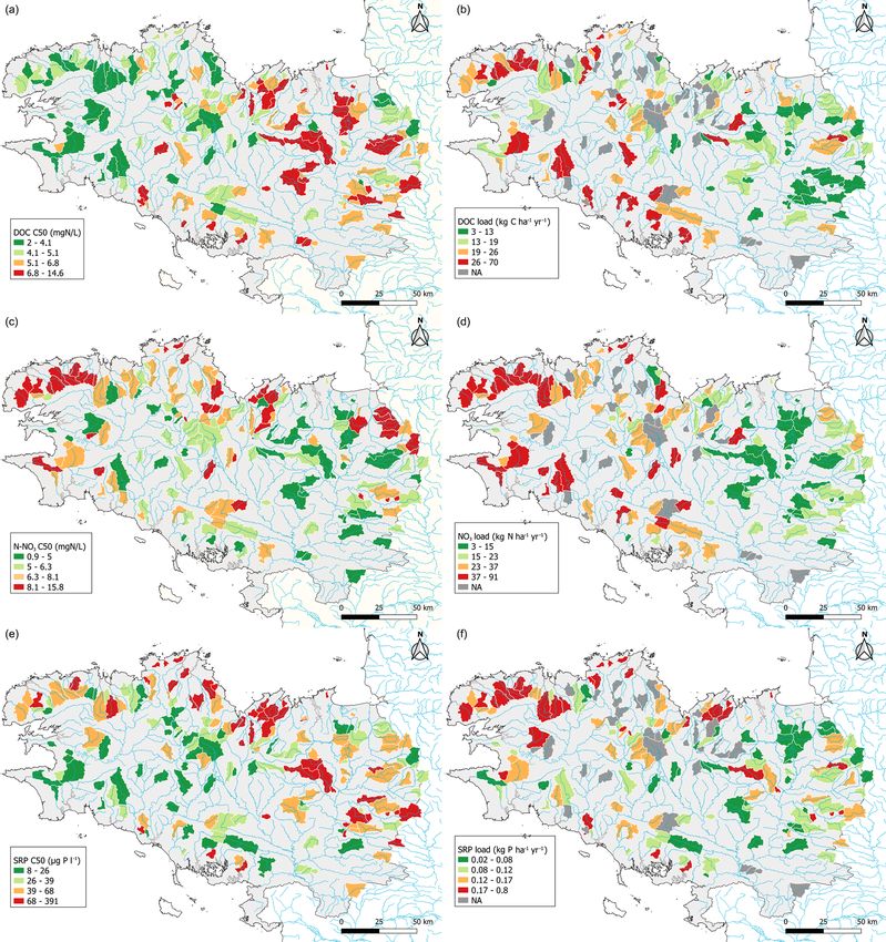
SRP 0.9207 0.4743 1.9412 Most of the catchments had a seasonal concentration cy-
cle: 85 %, 71 %, and 78 %, for NO3 , DOC, and SRP con-
centrations respectively, and 100 % of them had a seasonal
that concentrations varied less in space than in flow, and vice discharge cycle (Fig. 5). Means and SDs of the standard-
versa for SRP. ized Ampli were 0.59 ± 0.46 for NO3 , 0.53 ± 0.30 for DOC,
For DOC and NO3 , Ampli was not correlated significantly 0.79 ± 0.14 for SRP, and 1.99 ± 0.38 for discharge. The dis-
with C50, but it was with C90 (Figs. 4 and S8). For SRP, cor- tribution of the calculated seasonality indices is provided in
relations between Ampli and the percentiles were high, with Fig. S7.
rs > 0.85 for C50 and C90 (Figs. 4, S8). The SI and phases, The annual phases for discharge were more stable among
calculated on the catchments for which a GAM can be fitted, all catchments than those for concentrations. The highest
i.e. presenting a seasonal feature, were correlated more with discharge period was centred on mid-February (winter) and
C10 for DOC (n = 107) and NO3 (n = 98) (negatively for SI the lowest discharge period on September. A strong gradient
and positively for the phases), and more with C90 for SRP of hydrological dynamics was observed among catchments
(n = 118) (negatively, for SI only). (Figs. 5d and S7). The highest W 2 was associated with both
Mean (±1 SD) interannual loads had high spa- severe low-flow discharge and many high discharge events.
tial variabilities −20.71 ± 10.52 kg C ha−1 yr−1 for Values of Qmean , BFI, W 2, and QMNA clearly followed an
DOC, 27.48 ± 18.51 kg N ha−1 yr−1 for NO3 , and east–west gradient (not shown). Because of similar seasonal
0.315 ± 0.11 kg P ha−1 yr−1 for SRP – which differed discharge dynamics in all catchments, SI can be used to de-
from those observed for concentrations (Fig. 2). Unsurpris- scribe the seasonal dynamics of a concentration relative to
ingly, interannual loads of the three solutes were significantly those of discharge. When SI was positive, the concentration
(p < 0.001) and strongly correlated with annual water fluxes seasonality was in phase with discharge; when negative, the
(Pearson r = 0.88 for DOC, 0.90 for NO3 , and 0.75 for concentration seasonality was out of phase with discharge
SRP). There were weak but significant positive correlations (Fig. 5).
between mean interannual loads and seasonality indices Most of the catchments had opposite dynamics for DOC
(Ampli, SI) or C90 for DOC (Fig. 4). Mean interannual loads and NO3 . For 90 % of them, Pearson correlation between the
of NO3 were significantly and positively correlated with daily GAM estimates of DOC and NO3 was negative and
C10 and C50, and negatively with its seasonality indices. for 50 % of the catchments less than −0.79. The remaining
The strongest significant correlation was found between 10 % of catchments (15) had low Ampli of DOC and NO3 .
mean interannual loads and concentration percentiles for The DOC and NO3 concentrations had out-of-phase seasonal
SRP. cycles, as shown by the negative correlation between SI and
DOC or NO3 for all catchments that had a significant season-
3.2 Characterization of concentration seasonality ality in these concentrations (Fig. 6; R 2 = 0.62). We classi-
fied two types of catchments according to their seasonality in
3.2.1 Performance of GAMS both DOC (MinPhase) and NO3 (MaxPhase) concentrations
and consistent with the SI (Figs. 6, S7). NO3 MaxPhase and
Of the 185 catchments, GAMs were fitted for 159 to DOC DOC MinPhase that occurred before 1 May were classified
concentrations time series, 168 to NO3 concentrations time as “in phase” with discharge (Q), while those that occurred
series, 162 to SRP concentrations time series, and 185 to dis- after were “out of phase” with Q, as proposed by Van Me-
charge time series. The cases for which fitting was not possi- ter et al. (2019). All catchments experienced high stability
ble corresponded to those with no seasonal cyclicity or with of the DOC MaxPhase and NO3 MinPhase were the same
excessive interannual variability. The percentage of variance for all catchments as they always occurred between July and
explained by the GAM varied by site and solute. Fitting December (Figs. 5, S7).
performed best for NO3 , followed by SRP and then DOC: The first type, “in phase” (68 % of the catchments with
the means and SDs of the adjusted Rsq were 0.30 ± 0.18, seasonality), had a NO3 MaxPhase between October and
0.16±0.11, and 0.22±0.15 for NO3 , DOC, and SRP, respec- May (Figs. 5, S7) (i.e. high-flow period, in phase with maxi-
Hydrol. Earth Syst. Sci., 25, 2491–2511, 2021 https://doi.org/10.5194/hess-25-2491-2021S. Guillemot et al.: Spatio-temporal controls of C–N–P dynamics 2499 Figure 2. Map of median (a, c, e) concentrations C50 and (b, d, f) loads of dissolved organic carbon (DOC), nitrate N (N-NO3 ), and soluble reactive phosphorus (SRP) for the 185 streams. The catchments in grey did not meet the criteria to estimate a mean average interannual load. Classes in the legends have equal numbers of catchments. mum discharge and usually with DOC MinPhase). For these Phase between May and September (Figs. 5, S7) (i.e. low- catchments, the mean SI was positive for NO3 (0.22 ± 0.19) flow period, out of phase with maximum discharge). For and usually negative or null for DOC (0.00 ± 0.13). They most catchments, maximum NO3 and minimum DOC con- tended to be located toward central Brittany and be associ- centrations occurred a mean of 1.85 months before min- ated with mesoscale catchments (mean of 52.6 ± 38.8 km2 ). imum discharge or 5.5 months after maximum discharge, They had large Ampli for NO3 and low Ampli for DOC respectively. For these catchments, the mean SI was neg- (mean relative Ampli of 0.83 ± 0.46, and 0.44 ± 0.23 for ative or null for NO3 (−0.08 ± 0.06) and weakly positive DOC) and relatively low C50 of NO3 (means of 5.74 ± for DOC (0.21 ± 0.10). These catchments were close to the 2.46 mg N L−1 and 5.92 ± 2.00 mg C L−1 ). coast and relatively small (mean of 31.4 ± 21.7 km2 ). The The second type, “out of phase” (32 % of the catchments had smaller Ampli than “in-phase” catchments for NO3 , and with seasonality), had a DOC MinPhase and NO3 Max- higher Ampli for DOC (mean relative Ampli of 0.13 ± 0.13, https://doi.org/10.5194/hess-25-2491-2021 Hydrol. Earth Syst. Sci., 25, 2491–2511, 2021
2500                                                          S. Guillemot et al.: Spatio-temporal controls of C–N–P dynamics

Figure 3. (a) Principal component analysis of 10th, 50th, and 90th percentiles (C10, C50, and C90) of nitrate (N-NO3 ), dissolved organic
carbon (DOC), and soluble reactive phosphorus (SRP) concentrations for the 185 headwater catchments analysed. (b) Correlation between
the medians (C50) of DOC and N-NO3 concentrations for the 159 catchments in which DOC and NO3 were monitored from 2007–2017.
The colour gradient indicates the percentage of catchment area covered by summer crops.

Figure 4. Matrices of Spearman’s rank correlations of water quality (load, concentration percentiles (10th (C10), 50th (C50), and 90th
(C90)), and seasonality metrics) for (a) dissolved organic carbon (DOC), (b) nitrate N (N-NO3 ), and (c) soluble reactive phosphorus
(SRP) (c). Only significant (p ≤ 0.05) values are shown.

and 0.74 ± 0.30 for DOC) and relatively high C50 of NO3                3.3   Controlling factors of concentration and discharge
(means of 8.27 ± 2.90 mg N L−1 and 5.00 ± 1.62 mg C L−1 ).                   percentiles and seasonality
   Some catchments had intermediate behaviour between
these two types (Figs. 5 and 6). Some had a plateau with max-          The C50 of DOC was correlated significantly with 15 spatial
imum NO3 and minimum DOC concentrations from winter                    variables and most strongly (|rs | ≥ 0.4) with topographic in-
to summer, while others showed two maxima for NO3 or                   dex, QMNA, and the other hydrological indices. The C50 of
two minima for DOC (one synchronous with maximum dis-                  NO3 was correlated significantly with 12 spatial variables,
charge and another with minimum discharge). Other catch-               in particular diffuse agricultural sources (rs = 0.68 for the
ments also had maximum NO3 synchronous with discharge,                 percentage of summer crops, rs > 0.39 for N and P surplus,
but minimum DOC after maximum discharge.                               and rs = 0.48 for soil erosion rate) and hydrological indices,
   The seasonal dynamics of SRP were more stable than                  through the base flow index (BFI) (positively) and W 2 (neg-
those of DOC and NO3 , but less stable than those of dis-              atively) (Table 3). The C50 of SRP was correlated signif-
charge. Thus, there was only one type of seasonality for SRP,          icantly with more variables (18), but the correlations were
which was out of phase with flow: MaxPhase SRP dominated               slightly weaker. It correlated most strongly with soil P stock
in summer (mid-August ± 1.4 months), and MinPhase SRP                  (rs = −0.40), climate and hydrology (rs = −0.43 to −0.34
dominated in late winter (March ± 1.2 months) (Figs. 5, S6),           with effective rainfall, Qmean, QMNA), elevation, and hy-
except for two catchments with maximum SRP in January–                 drographic network density. It had weaker positive correla-
February.                                                              tions (rs < 0.3) with the soil erosion rate and domestic and
                                                                       agricultural pressures (urban percentage and P surplus).

Hydrol. Earth Syst. Sci., 25, 2491–2511, 2021                                           https://doi.org/10.5194/hess-25-2491-2021
S. Guillemot et al.: Spatio-temporal controls of C–N–P dynamics 2501 Figure 5. Seasonal dynamics of (a) nitrate N (N-NO3 ), (b) dissolved organic carbon (DOC), (c) soluble reactive phosphorus (SRP), and (d) daily discharge modelled by generalized additive models, for 185 headwater catchments. To compare concentrations, they are standard- ized by their mean interannual concentration. The colour gradient represents the seasonality index of each parameter; thus, a headwater catchment’s colour can vary among panels. Ampli and SI for DOC and NO3 were correlated most with Discharge indicators present some obvious correlations (e.g. the hydrodynamic properties, followed by agricultural pres- Q50 and annual amplitude with Qmean and QMNA). Q50 sures (Fig. 7, Table 3). The catchments “in phase” with dis- and, in a lower degree, annual amplitude are positively cor- charge (i.e. positive SI–NO3 and negative SI–DOC correla- related with baseflow index (BFI) and negatively correlated tions) were associated with high hydrological reactivity (low with flow flashiness (W 2). This indicates that in catchments BFI and high W 2) and a low percentage of summer crops where streams are more influenced by groundwater (gener- (Table 3). Conversely, catchments “out of phase” with dis- ally those flowing on granite), BFI is high and flow flashiness charge (i.e. negative SI–NO3 and positive SI–DOC correla- is low. tions) were associated with low hydrological reactivity (high Correlations with catchment characteristics are lower than BFI and QMNA, low W 2) and a high percentage of summer expected for the Q50. Q50 is significantly correlated with crops. wetness topographic index (meanTWI, rs = −0.53), which Correlations of SI with catchment descriptors were weaker indicates that Q50 is increasing in catchments with drier (|rs | ≤ 0.4) for SRP than for DOC, NO3 , and discharge be- soils (meanTWI low). Positive correlation with granite indi- cause most catchments had the same seasonal pattern, with cates that discharge is more supported by this type of rocks, maximum SRP concentration during low flow. Catchments which present favourable groundwater storage. Q50 is pos- with the highest amplitudes of SRP concentration were asso- itively correlated with soil TP, which is higher on granite ciated with low QMNA and Qmean, high W 2, low effective substratum. Q50 is positively correlated with SummerCrop rainfall, and low soil P stock. Interannual loads were corre- and negatively with WinterCrop, underlying higher runoff in lated mainly with hydrological descriptors (positively with catchments with non-cultivated soil during winter. Qmean and QMNA, and negatively with W 2) (Table 3). In- terannual NO3 loads were also correlated with the percentage of summer crops and soil TP content, while interannual SRP loads were correlated weakly with the percentage of sum- mer crops, agricultural surplus, erosion, and point sources. https://doi.org/10.5194/hess-25-2491-2021 Hydrol. Earth Syst. Sci., 25, 2491–2511, 2021
2502                                                                       S. Guillemot et al.: Spatio-temporal controls of C–N–P dynamics

Table 3. Spearman rank correlations between water quality indices for dissolved organic carbon (DOC), nitrate (NO3 ), soluble reactive
phosphorus (SRP), discharge indices (Q), and geographical descriptors. Only significant correlations (p ≤ 0.05) are shown, and bold text
indicates |r| ≥ 0.40.

                                                      DOC                              NO3                              SRP                          Q
    Spatial variable                       C50    Ampli       SI   Load     C50    Ampli       SI   Load     C50    Ampli      SI    Load     Q50        Ampli
    Topography            Area                –   −0.24        –       –       –       –        –       –       –       –        –       –       –           –
                          Elevation       −0.46   −0.18        –       –       –   −0.31     −0.2    0.19    −0.2       –        –    0.38    0.38        0.37
                          Density_hn          –       –        –       –       –   −0.22        –    0.16    −0.3   −0.27     0.19    0.25    0.25           –
                          meanTWI          0.54       –        –       –       –    0.41     0.25   −0.33    0.39    0.25        –   −0.53   −0.53       −0.59
                          IDPR                –       –        –       –       –       –        –       –   −0.21   −0.19        –     0.2     0.2           –
    Geology               Granite_pm          –       –    0.21     0.41       –   −0.43   −0.31     0.27   −0.26   −0.24       –     0.43    0.43        0.35
                          Schist_pm           –   −0.21   −0.37    −0.29   −0.16    0.25    0.22    −0.23       –       –       –    −0.25   −0.25           –
                          Other_pm            –    0.32    0.35        –    0.28       –       –        –    0.28    0.16       –        –       –           –
    Soil                  Erosion         −0.36    0.24        –       –    0.48    0.16   −0.26     0.39    0.24    0.17       –        –       –           –
                          OC_soil         −0.27   −0.21        –       –       –   −0.29       –     0.18    −0.2   −0.19       –     0.34    0.34        0.32
                          TP_soil         −0.44       –        –    0.38       –   −0.51   −0.34     0.49    −0.4   −0.32       –     0.78    0.78        0.71
    Land use              SummerCrop      −0.3     0.28     0.54       –    0.68       –   −0.47     0.54       –       –    0.29     0.29    0.29           –
                          WinterCrop      0.19        –     −0.2   −0.29       –    0.48    0.21    −0.23    0.17       –   −0.18    −0.51   −0.51       −0.34
                          Forest             –    −0.17     −0.3    0.23   −0.37   −0.47       –        –   −0.29   −0.19       –        –       –        0.25
                          Pasture            –        –        –       –    −0.3       –    0.26     −0.2       –       –       –        –       –           –
                          Urban              –        –        –       –       –       –       –        –    0.23       –       –        –       –           –
    N and P diffuse and   N_surplus       −0.21     0.2        –       –    0.39       –       –     0.38       –       –     0.29    0.28    0.28           –
    point sources         P_surplus       −0.24    0.33        –   −0.22    0.49       –   −0.32     0.37     0.2   −0.19        –     0.2     0.2           –
                          N_point             –   −0.17        –       –       –       –       –        –       –       –        –       –       –           –
                          P_point             –   −0.16        –       –       –       –       –     0.21       –       –        –       –       –           –
    Hydrology             Qmean           −0.49    0.19       –     0.53    0.16   −0.58   −0.42     0.67   −0.39   −0.31    0.21     0.95    0.95        0.9
                          QMNA            −0.52    0.25    0.41     0.48    0.42   −0.54   −0.56     0.76   −0.34   −0.32    0.35     0.94    0.94        0.7
                          BFI             −0.41   −0.27    0.64     0.38    0.54   −0.52   −0.69     0.57    −0.2   −0.23    0.32     0.72    0.72       0.21
                          W2               0.43       –   −0.61    −0.46   −0.49    0.54    0.68    −0.59     0.2     0.2   −0.26    −0.76   −0.76       −0.3
                          Precipitation    −0.5       –       –     0.47       –    −0.6   −0.39      0.6   −0.43   −0.33    0.18     0.88    0.88       0.86
                          Wetland          0.16       –    0.31     0.38       –       –       –        –       –       –       –        –       –          –

4      Discussion                                                                   Hedin et al., 1998; Hill et al., 2000) suggested that DOC
                                                                                    supply limits in- and near-stream denitrification. In contrast,
4.1        Interpretation of the spatial opposition between                         other studies claimed that N can influence loss of DOC from
           DOC and NO3                                                              soils by altering substrate availability or/and microbial pro-
                                                                                    cessing of soil organic matter (Findlay, 2005; Pregitzer et al.,
Spatial opposition between DOC and NO3 concentrations                               2004). In our study, C50 was correlated with both BFI and
has been reported for a wide range of ecosystems. Taylor                            QMNA, positively for NO3 and negatively for DOC, which
and Townsend (2010) found a non-linear negative relation-                           suggests that catchments strongly sustained by groundwa-
ship between them for soils, groundwater, surface freshwa-                          ter flow produced higher NO3 and lower DOC concentra-
ter, and oceans, from global to local scales, and highlighted                       tions, as reported in other rural catchments (e.g. Heppell et
that this negative correlation prevails in disturbed ecosys-                        al., 2017). The C50 of NO3 increased with agricultural pres-
tems. Goodale et al. (2005) reported a similar negative cor-                        sures (percentage of summer crop, N surplus), as observed
relation among 100 streams in the northeastern USA. Hep-                            by Lintern et al. (2018), while that of DOC increased in flat-
pell et al. (2017) found that DOC and NO3 concentrations                            ter catchments, which is consistent with results of Mengistu
were inversely correlated with the BFI in six reaches of the                        et al. (2014) and Musolff et al. (2018).
Hampshire Avon catchment (UK). Our contribution brings                                 This suggests that this spatial opposition between DOC
an original focus on this relationship in headwater catch-                          and NO3 results from the combination of heterogeneous hu-
ments with high domestic and agricultural pressures. Tay-                           man inputs, heterogeneous natural pools, and different physi-
lor and Townsend (2010) interpreted this spatial opposition                         cal and biogeochemical connections between C and N pools.
as a response of microbial processes (i.e. biomass produc-                          In surface water, these heterogeneous sources are expressed
tion, nitrification, and denitrification) to the ratio of ambient                   to differing degrees depending on the catchment’s hydrolog-
DOC : NO3 , which controls NO3 export/retention in catch-                           ical behaviour. When deep or slow flow paths dominate, they
ments (see also Goodale et al., 2005). In semi-natural ecosys-                      store and release N via groundwater and mobilize little the
tems, high but poorly labile soil organic C pools were as-                          sources rich in organic matter. When shallower and faster
sociated with lower N retention capacity and thus higher N                          flow paths dominate, they transport some of the N via com-
leaching (Evans et al., 2006). Similarly, several studies (e.g.

Hydrol. Earth Syst. Sci., 25, 2491–2511, 2021                                                           https://doi.org/10.5194/hess-25-2491-2021
S. Guillemot et al.: Spatio-temporal controls of C–N–P dynamics 2503
crease. These reactions consume NO3 (e.g. denitrification,
biological uptake) and release (reductive dissolution) or pro-
duce (autotrophic production) DOC. Of the two seasonal
NO3 –DOC cycles, the most common in our datasets is thus
maximum NO3 in phase with maximum discharge and min-
imum DOC, which has been reported in Brittany (Abbott
et al., 2018b; Dupas et al., 2018) and elsewhere (Van Me-
ter et al., 2019; Dupas et al., 2017; Halliday et al., 2012;
Minaudo et al., 2015; Weigand et al., 2017). The main con-
trol of seasonal DOC–NO3 cycles appears to be related to hy-
drological indices (expressed as BFI and W 2). Hydrological
flashiness reflects the relative importance of subsurface flow
compared to deep base flow (Heppell et al., 2017); thus, low
BFI (or high W 2) would indicate higher connectivity with
subsurface riparian sources and shorter transit times. This
is consistent with results of Weigand et al. (2017), who ob-
served higher seasonal amplitudes in DOC and NO3 concen-
trations and stronger temporal anti-correlation between DOC
and NO3 concentrations in stream water dominated by sub-
surface runoff.
Our results are consistent with these previous results,
Figure 6. Relationship between the seasonality indices (SI) of ni- while the correlations with catchment characteristics can pro-
trate N (N-NO3 ) vs. dissolved organic carbon (DOC) in the headwa- vide some explanation. Catchments with low BFI have larger
ter catchments for which seasonality was significant for both param- shallow flows and experience seasonal DOC–NO3 cycles that
eters (n = 98). The colour and shape of symbols identify the season- are in phase with flow and have higher NO3 amplitudes.
ality types based on the NO3 MaxPhase and DOC MinPhase met- These cycles can be interpreted as the combination of sev-
rics. The threshold date was 1 May: MaxPhase metrics that occurred eral mechanisms (Fig. 8):
before were classified as “in phase” with discharge (Q), while those
that occurred after were “out of phase” with Q. The DOC MinPhase 1. synchronization (i.e, coincident timing) of NO3 -rich
metric is shown to highlight the synchrony between minimum DOC and DOC-poor groundwater contribution with maxi-
and maximum N-NO3 concentrations.
mum flow;
2. large contribution of near-/in-stream biogeochemical
partments rich in organic matter, which causes N depletion processes at reduced low flows that decreases NO3 con-
and release of more DOC to the streams. The initial amounts centration (e.g. NO3 consumption by aquatic microor-
of NO3 along these flow paths are a function of human pres- ganisms, biofilms, macrophytes, and redox processes);
sures.
3. large DOC-rich riparian contribution throughout the
4.2 Interpretation of the temporal opposition between year but larger in autumn, when flow starts to increase,
DOC and NO3 as described in detail in previous AgrHys Observatory
studies (Aubert et al., 2013; Humbert et al., 2015).
The seasonal opposition between DOC and NO3 concentra-
tion dynamics could be another manifestation of the spa- In contrast, catchments with higher BFI have smaller shal-
tial opposition between DOC and NO3 sources, because the low flows and experience mainly DOC and NO3 cycles that
strength of the hydrological connection between sources and are out of phase with flow and have lower amplitudes. These
streams varies seasonally (e.g. Mulholland and Hill, 1997; cycles can be attributed to the following:
Weigand et al., 2017). The direct contribution of biogeo-
chemical reactions that connect DOC and NO3 cycles may 1. The groundwater contribution is more continuous, com-
also vary seasonally (Mulholland and Hill, 1997; Plont et bined with a decrease in agricultural pressures over
al., 2020). Indeed, temperature, wetness condition, and light time, and consequently a decrease of NO3 concen-
availability influence rates of these organic matter reactions tration in shallower/younger groundwater than in the
(Davidson et al., 2006; Hénault and Germon, 2000; Luo and deeper/older one (Abbott et al., 2018b; Martin et al.,
Zhou, 2006). In addition, the relative importance of the fluxes 2004, 2006). This vertical gradient in groundwater sup-
produced or consumed via these reactions appears clearer ply could explain why NO3 concentrations peaked dur-
during the low-flow period, when the fluxes exported from ing the annual discharge recession, which is sustained
the terrestrial ecosystem and delivered to the stream de- mainly by deep groundwater inputs.
https://doi.org/10.5194/hess-25-2491-2021 Hydrol. Earth Syst. Sci., 25, 2491–2511, 20212504 S. Guillemot et al.: Spatio-temporal controls of C–N–P dynamics
Figure 7. Relationship between the seasonality index (SI) of dissolved organic carbon (DOC) and nitrate (NO3 ) and the hydrological
reactivity descriptors (a) flow flashiness index (W 2) and (b) base-flow index (BFI) for 124 headwater catchments.
2. There is little contribution of near-/in-stream biogeo- livestock production (Sharpley et al., 1994). This led to cor-
chemical processes at reduced low flows due to larger relations between soil P and runoff concentrations in agri-
inputs from groundwater, which maintains a relatively cultural catchments (Cooper et al., 2015; Sandström et al.,
high minimum NO3 concentration. 2020), as found here.
The seasonality of SRP was generally the same in the re-
3. Contributions of DOC-rich riparian sources, mainly in gion studied, and C50 and amplitudes were significantly cor-
autumn, are smaller than those in in-phase catchments, related. A peak in seasonal SRP concentrations at low flow
again due to a predominantly deeper geometry of water has been reported previously (Abbott et al., 2018b; Bowes et
circulation. al., 2015; Dupas et al., 2018; Melland et al., 2012). It is inter-
preted as the result of a dominance of point sources diluted
during high flow (Minaudo et al., 2015, 2019; Bowes et al.,
4.3 Interpretation of the spatial and temporal 2011) or of stream-bed sediment sources for which P release
signature of SRP increases with temperature (Duan et al., 2012).
Correlation between spatial patterns of NO3 and SRP was
The correlations between the C50 of SRP and geographic expected given the dominant agricultural origin of N and sub-
variables highlighted the importance of P sources (soil P stantial agricultural origin of P, but it was not observed in all
stocks, followed by domestic and agricultural pressures) and catchments. The C50 of NO3 and SRP was high mainly on
surface flow paths (e.g. hydrological indices, elevation, ero- the northwestern coast, perhaps due to intensive vegetable
sion risk). Similarly, analysis of regression models that pre- production associated with a dominance of mineral fertiliza-
dicted spatial variability in total P concentration of 102 ru- tion (Lemercier et al., 2008). Elsewhere, a high proportion of
ral catchments in Australia also indicated positive effects of allochthonous P in the topsoil results from livestock farm-
human-modified land uses, natural land uses prone to soil ing and manure application (Delmas et al., 2015). The P-
erosion, mean P content of soils, and to a lesser extent, to- retention capacity of soils (related to their Al, Ca, Fe, and
pography (Lintern et al., 2018). They always included the clay contents) is also likely to increase spatial variability in
percentage of urban area, which suggests a considerable ef- the release of P from catchments (Delmas et al., 2015). Syn-
fect of sewage discharge, even at low levels of urbanization. chronous variations in SRP and DOC, such as those observed
The catchments analysed in the present study have a homo- in small, completely agricultural headwater catchments with-
geneous and relatively dense distribution of small villages out villages (Cooper et al., 2015; Dupas et al., 2015b; Gu
but no large city, which seems to support this last hypothesis. et al., 2017), were not observed in the present set of catch-
Sobota et al. (2011) studied spatial relationships among P in- ments. We assume that synchronicity of SRP and DOC in
puts, land cover, and mean annual concentrations of different small catchments depends on soil processes, such as reduc-
forms of P in 24 catchments in California, USA. They found tion of soil Fe oxyhydroxides in wetland zones (Gu et al.,
that P concentrations were significantly correlated with agri- 2019), which are hidden by in-stream processes (P adsorp-
cultural inputs and, to a lesser extent, agricultural land cover tion on streambed sediments) and downstream point-source
but not with estimates of sewage discharge. Nonpoint sources inputs (especially P inputs) in the set of larger catchments
of P in agricultural runoff, historical inputs of fertilizer and studied.
manure in excess of crop requirements, have led to a build-
up of soil P levels, particularly in areas of intensive crop and
Hydrol. Earth Syst. Sci., 25, 2491–2511, 2021 https://doi.org/10.5194/hess-25-2491-2021You can also read