An unsupervised learning approach to identifying blocking events: the case of European summer
←
→
Page content transcription
If your browser does not render page correctly, please read the page content below
Weather Clim. Dynam., 2, 581–608, 2021
https://doi.org/10.5194/wcd-2-581-2021
© Author(s) 2021. This work is distributed under
the Creative Commons Attribution 4.0 License.

An unsupervised learning approach to identifying
blocking events: the case of European summer
Carl Thomas1 , Apostolos Voulgarakis1,2 , Gerald Lim3 , Joanna Haigh1,4 , and Peer Nowack1,4,5,6
1 Department  of Physics, Imperial College London, South Kensington Campus, London, SW7 2BW, UK
2 School of Environmental Engineering, Technical University of Crete, Chania, Crete, 73100, Greece
3 Centre for Climate Research Singapore, 36 Kim Chuan Road, 537054, Singapore
4 Grantham Institute, Imperial College London, SW7 2AZ, UK
5 Climatic Research Unit, School of Environmental Sciences, Norwich, NR4 7TJ, UK
6 Data Science Institute, Imperial College London, South Kensington Campus, London, SW7 2AZ, UK

Correspondence: Carl Thomas (c.thomas18@imperial.ac.uk)

Received: 11 January 2021 – Discussion started: 14 January 2021
Revised: 3 June 2021 – Accepted: 4 June 2021 – Published: 12 July 2021

Abstract. Atmospheric blocking events are mid-latitude             events, although the domain-based approach can still lead to
weather patterns, which obstruct the usual path of the po-         errors in the identification of certain events in a fashion simi-
lar jet streams. They are often associated with heat waves         lar to the other BIs. We further test the red blocking detection
in summer and cold snaps in winter. Despite being central          skill of SOM-BI depending on the meteorological variable
features of mid-latitude synoptic-scale weather, there is no       used to study blocking, including geopotential height, sea
well-defined historical dataset of blocking events. Various        level pressure and four variables related to potential vorticity,
blocking indices (BIs) have thus been suggested for auto-          and the 500 hPa geopotential height anomaly field provides
matically identifying blocking events in observational and in      the best results with our new approach. We also demonstrate
climate model data. However, BIs show significant regional         how SOM-BI can be used to identify different types of block-
and seasonal differences so that several indices are typically     ing events and their associated trends. Finally, we evaluate
applied in combination to ensure scientific robustness. Here,      the SOM-BI performance on around 100 years of climate
we introduce a new BI using self-organizing maps (SOMs),           model data from a pre-industrial simulation with the new
an unsupervised machine learning approach, and compare its         UK Earth System Model (UKESM1-0-LL). For the model
detection skill to some of the most widely applied BIs. To         data, all blocking detection methods have lower skill than for
enable this intercomparison, we first create a new ground          the ERA5 reanalysis, but SOM-BI performs noticeably bet-
truth time series classification of European blocking based        ter than the conventional indices. Overall, our results demon-
on expert judgement. We then demonstrate that our method           strate the significant potential for unsupervised learning to
(SOM-BI) has several key advantages over previous BIs be-          complement the study of blocking events in both reanalysis
cause it exploits all of the spatial information provided in the   and climate modelling contexts.
input data and reduces the dependence on arbitrary thresh-
olds. Using ERA5 reanalysis data (1979–2019), we find that
the SOM-BI identifies blocking events with a higher preci-
sion and recall than other BIs. In particular, SOM-BI already      1   Introduction
performs well using only around 20 years of training data so
that observational records are long enough to train our new        Atmospheric blocking events are large-scale mid-latitude an-
method. We present case studies of the 2003 and 2019 Eu-           ticyclones that can persist for several days, which obstruct the
ropean heat waves and highlight that well-defined groups of        typical westerly flow pattern (Rex, 1950). Blocking systems
SOM nodes can be an effective tool to diagnose such weather        are often associated with regional extreme weather events,
                                                                   particularly heat waves in summer and cold snaps in winter.

Published by Copernicus Publications on behalf of the European Geosciences Union.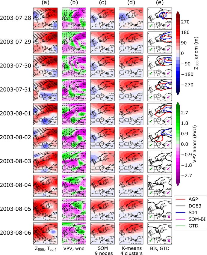
582                                     C. Thomas et al.: An unsupervised learning approach to identifying blocking events

For example, the 2003 summer heat wave and 2009/10 win-                 With the advent of modern computational methods, ex-
ter cold events in Europe were both associated with atmo-            tensive study of the available record of surface analyses to
spheric blocking (Black et al., 2004; Cattiaux et al., 2010).        identify blocking events no longer requires a prohibitive ex-
The evolution of atmospheric blocking itself is nonlinear            penditure of time. Here, we therefore define a new binary
(Palmer, 1999), and the underlying complex physical mech-            ground truth dataset (GTD) of European blocking events
anisms are not yet fully understood (Nakamura and Huang,             across June–July–August (JJA) 1979–2019, based on a 5 d
2018; Woollings et al., 2018). There is a large seasonal, inter-     threshold, reanalysis data and expert judgement. Our under-
annual and decadal variability in the occurrence of blocking         standing of blocking events has been informed by the BIs and
(Kennedy et al., 2016; Brunner et al., 2017), which com-             the various definitions that have been proposed, but we do not
pounds the problem of separating externally forced changes           rely on any BIs for our study. This enables an independent
from internal variability (Barnes et al., 2014; Shepherd,            time series comparison with the BIs. We also compare our
2014). As a result, the influence of climate change on block-        results to a K-means clustering approach to describing the
ing remains an open question (Francis and Vavrus, 2012;              weather regimes of the mid-latitude atmosphere. We present
Barnes, 2013; Hassanzadeh et al., 2014; Barnes and Polvani,          case studies of the prominent 2003 and 2019 European heat
2015; Barnes and Screen, 2015; Francis and Vavrus, 2015;             waves, where we show how well K-means clustering, the BIs
Coumou et al., 2018; Mann et al., 2018).                             and SOMs describe the blocking events.
   In order to better understand blocking and to investigate            We then use SOMs to develop a new blocking index
the influence of climate change, there have been signifi-            (SOM-BI, pronounced “zombie”). This SOM-BI method has
cant efforts to develop methods that can automatically detect        advantages over previous BIs because it exploits all the spa-
blocking in long meteorological records. Since “any attempt          tial information provided in the input data and reduces the
to identify blocked cases with certainty from an inspection          dependence on arbitrary thresholds. It also provides a new
of the longer available record of surface analyses would re-         way of studying blocking events that can more intuitively
quire a prohibitive expenditure of time” (Rex, 1950), block-         distinguish between different regimes and locations of block-
ing indices (BIs) have been developed to objectively identify        ing events, which the other indices are lacking. We identify
blocked events (Lejenäs and Økland, 1983; Dole and Gor-              the skill of different BIs by developing a binary time series
don, 1983; Tibaldi and Molteni, 1990; Pelly and Hoskins,             identification of European blocking patterns and comparing
2003). However, the multiplicity of these BIs, with a variety        this to our GTD using standard skill metrics discussed in
of thresholds for defining the area, persistence and magni-          Sect. 2.6. This study is the first to define a GTD, and we use
tude of blocked features on different atmospheric dynami-            it as a benchmark to compare the skill of different BIs over a
cal variables, means that these methods necessarily carry the        region.
burden of somewhat subjective definitions. Notably, while               As a key result, we find that through comparison with
previous intercomparisons of BIs show similar global clima-          three BIs used in a recent inter-comparison study (Pinheiro
tologies, and while all indices capture many of the basic fea-       et al., 2019), the SOM-BI method has an improved skill at de-
tures of atmospheric blocking within their definitions, there        tecting regional blocking events. Since the SOM-BI method
are known regional and seasonal differences (Croci-Maspoli           is not bound to a specific meteorological variable, we also
et al., 2007; Barriopedro et al., 2010; Pinheiro et al., 2019). In   quantify how its detection skill varies with the variable used,
addition, whilst spatial climatologies obtained from these BIs       from geopotential height anomaly fields to potential vortic-
have been compared extensively, to the best of our knowl-            ity maps. While there have been theoretical discussions on
edge there has been no direct time series comparison of the          the importance of the meteorological variable used to define
BIs beyond case study analyses such as those in Scherrer             and identify blocking (Pelly and Hoskins, 2003; Chen et al.,
et al. (2006) and Pinheiro et al. (2019).                            2015), the variable dependence of skill of blocking detection
   Other frequently used methods to study the climatology            methods has not been quantified before. Finally, we evalu-
and characteristics of blocking include K-means clustering           ate the performance of SOM-BI on 41 years from the ERA5
analyses to study weather regimes (Vautard, 1990; Michelan-          reanalysis and 101 years of a pre-industrial control run car-
geli et al., 1995; Cassou, 2008; Ullmann et al., 2014; Strom-        ried out with the UK Earth System Model (UKESM1-0-LL,
men et al., 2019; Fabiano et al., 2021) and an unsuper-              hereafter UKESM). We identify a moderate improvement in
vised machine learning approach called self-organizing maps          blocking identification over the BIs for the reanalysis period
(SOMs) (Skific and Francis, 2012; Horton et al., 2015; Mio-          and a significant improvement for the UKESM data. A key
duszewski et al., 2016; Gibson et al., 2017a). It has been           advantage is that the longer climate model simulation allow
highlighted that consistency across various methods in de-           us to test the robustness of our method compared to other BIs
tecting long-term changes is a fundamental requirement to            over longer timescales, as well as to study the dependence of
confidently identify trends (Barnes et al., 2014; Woollings          the SOM-BI detection skill on the number of years included
et al., 2018). To the best of our knowledge, there has been          in the algorithm’s training dataset.
no previous study that directly compared a SOM approach to              Our paper is structured as follows. In Sect. 2 and its sub-
other BIs.                                                           sections, we introduce the meteorological reanalysis and cli-

Weather Clim. Dynam., 2, 581–608, 2021                                                  https://doi.org/10.5194/wcd-2-581-2021
C. Thomas et al.: An unsupervised learning approach to identifying blocking events                                            583

mate model data, the new GTD, the BIs, K-means clustering,        with the tropopause in the mid-latitude summer, as shown
SOMs, and our new SOM-BI. In Sect. 3, we present the main         in Fig. 1 of Liniger and Davies (2004), and therefore repre-
results of our analysis. We first compare the various blocking    sent upper-level dynamics. For the case study analyses we
identification methods by means of the 2003 and 2019 Euro-        have also used the surface horizontal wind fields and surface
pean heat wave case studies (Sect. 3.1), followed by an eval-     temperature (Tsurf ).
uation and intercomparison of the methods on ERA5 reanal-            Following Grotjahn and Zhang (2017) and Pinheiro et al.
ysis and UKESM climate model data (Sects. 3.2 and 3.3). In        (2019), we define the anomaly fields that we study by sub-
Sect. 3.4, we discuss how the performance of our new SOM-         tracting a long-term daily mean (LTDM) from the data in-
BI depends on the length of the data record used to train the     stead of subtracting the daily average. This is a smoothed
algorithm. In Sect. 3.5, we test the feasibility to train SOM-    function of the 365 d seasonal cycle across Z500 , VPV and
BI on ERA5 data to then reliably identify blocking in climate     Tsurf using the first six harmonics of their Fourier series,
model data, and vice versa. In Sect. 3.6 we briefly discuss       where the first harmonic corresponds to the mean and the
the effect of other hyperparameters on the SOM-BI skill. In       fifth to a 73 d span. The purpose of this is to smooth out the
Sect. 3.7, we demonstrate how SOM-BI can be used to study         daily mean fields, which can otherwise show excessive vari-
trends in regional blocking patterns by applying it to ERA5       ation between neighbouring days across the seasonal cycle.
data. In Sect. 4, we summarize and discuss our key results           The Tsurf and Z500 anomaly fields in ERA5 have been de-
and propose avenues for future work, especially concerning        trended linearly across time to remove the effect of thermo-
the detection of blocking in climate change simulations.          dynamic warming. Following Jézéquel et al. (2017) we sub-
                                                                  tract a spatially uniform trend, so that the horizontal gradients
                                                                  of the field are not altered. We depart from the Jézéquel et al.
2     Methods                                                     (2017) method by subtracting a linear Z500 anomaly trend
                                                                  instead of a cubic spline interpolation, since we assume that
2.1    Meteorological data                                        in the 1979–2019 time period the thermodynamic dilation of
                                                                  the troposphere can be approximated as linear, so removing
As a proxy for observed dynamical states over Europe,             nonlinear trends could risk removing the dynamical changes
we used ERA5 reanalysis data from the European Centre             in the atmosphere that we are interested in. We also apply the
for Medium Range Weather Forecasts (ECMWF, Hersbach               same detrending approach to the pre-industrial UKESM data
et al., 2020). The pre-industrial climate model data was          to remove any minor remaining trends in the data, e.g. due
obtained from simulations carried out with the UK Earth           to the finite spin-up time of the control simulations (Gregory
System Model UKESM1-0-LL (UKESM), as part of Cou-                 et al., 2004; Nowack et al., 2017; Mansfield et al., 2020).
pled Model Intercomparison Project Phase 6 (CMIP6, Eyring
et al., 2016; Sellar et al., 2019). For ERA5, we used grid-       2.2   Creating the ground truth dataset (GTD)
ded data at a spatial resolution of 1◦ × 1◦ across 1979–2019
and created daily averages derived from 3-hourly intervals.       In order to objectively compare the blocking indices, we de-
In UKESM, we used 101 years of daily data from the pre-           velop a ground truth dataset (GTD) of blocking events in
industrial run of the r1i1p1f2 ensemble member, across the        JJA Europe, here defined as 30–75◦ N, 10◦ W–40◦ E, fol-
arbitrarily defined 1960–2060 period. We used the UKESM           lowing IPCC AR5 definitions (Stocker et al., 2013). The
data at the native resolution of 1.25◦ × 1.875◦ to develop        northern latitude is extended to 76◦ N when using data on
the GTD plots and regridded to a 2◦ × 2◦ grid for the SOM         a 2◦ × 2◦ grid. JJA Europe was chosen because of our inter-
analysis. When training and testing between the ERA5 and          est in the role of atmospheric dynamics in the development
UKESM data (Sect. 3.5), we also regridded the ERA5 data           of mid-latitude land heat waves. Europe is a region which has
to a 2◦ × 2◦ grid.                                                seen many recent significant heat extremes (Christidis et al.,
   For both types of datasets, we used the following common       2014), and the role of changes in atmospheric dynamics has
meteorological variables to characterize the dynamical state      been a significant area of interest (Cattiaux et al., 2013; Hor-
of the atmosphere at any given time: geopotential height at       ton et al., 2015; Saffioti et al., 2017; Huguenin et al., 2020).
500 hPa (Z500 ), mean sea level pressure (MSLP) and relative         The GTD has been derived by studying every successive
vorticity at 500 hPa (ζ500 ). For ERA5, we also used vertically   5 d period from 28 May 1979 to 4 September 2019 and man-
integrated potential vorticity across 150–500 hPa (VPV),          ually identifying whether or not a blocking high persisted
isentropic potential vorticity on 350 and 330 K (IPV350 and       across any such 5 d period. By including the last 4 d at the
IPV330 ), and potential temperature on the PV = 2 PVU sur-        end of May and the first 4 d of September, we ensure that we
face (θ -PV). These PV-based variables have all been used in      capture all blocking events within the JJA period. A period
the context of understanding atmospheric blocking (Hoskins        of 5 d was chosen since this a typical persistence threshold
et al., 1985; Crum and Stevens, 1988; Pelly and Hoskins,          for blocking indices (Verdecchia et al., 1996; Schwierz et al.,
2003) but are not available from the CMIP6 archive. The 350       2004; Scherrer et al., 2006; Pinheiro et al., 2019), although
and 330 K isentropes were chosen because these intersect          a persistence of 7–10 d with weaker BI thresholds for am-

https://doi.org/10.5194/wcd-2-581-2021                                              Weather Clim. Dynam., 2, 581–608, 2021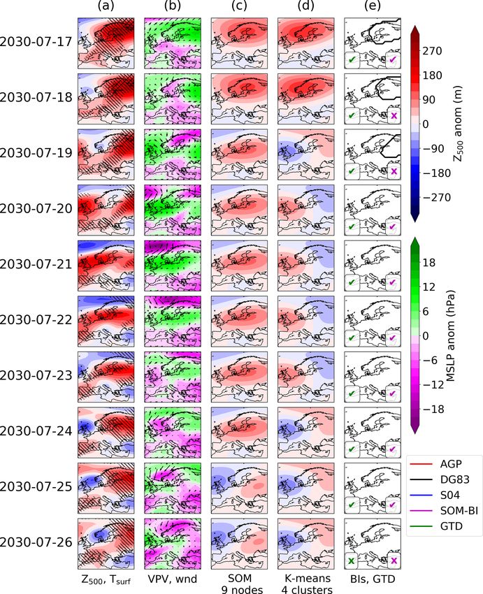
584 C. Thomas et al.: An unsupervised learning approach to identifying blocking events
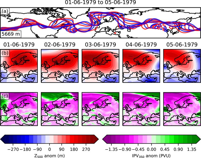
Figure 1. The information used to classify blocks in the ERA5 ground truth dataset (GTD). Panel (a) shows the Z500 contour for the averaged
value across 30–70◦ N, indicated in the bottom left of the panel. The red and blue colours highlight the contours at midnight and midday
respectively. Panels (b) and (c) show the Z500 time detrended anomaly and IPV350 anomaly for each day.
plitude and area has also been used (Rex, 1950; Lejenäs and in Fig. A1. As in Fig. 1, there is a clear quasi-stationary high
Økland, 1983). centred on a region slightly north of the UK. This is indi-
A diagram of the type of information analysed to label cated by the Z500 contours which show a significant north-
each individual day is shown in Fig. 1, for the example period ward protrusion over this region and by the substantial Z500
1–5 June 1979. This period was labelled as blocked, since anomaly across all panels in Fig. 1b. Since PV is not avail-
Fig. 1a clearly shows a continuous north shift in the Z500 able in CMIP6 data and the physical variables used to derive
contours over Europe and Fig. 1b shows a substantial pos- PV are not available at sufficiently high vertical resolution,
itive Z500 anomaly which persists across northern Europe. we instead show the MSLP anomaly field in Fig. A1c, which
The IPV350 maps in Fig. 1c highlight filaments and regions also indicates a high-pressure region consistent with Fig. A1a
where there is fast moving air. Once the total set of all 4001 and b.
consecutive 5 d periods across JJA 1979–2019 has been clas-
sified, persistent blocking events are reconstructed to form 2.3 Blocking indices (BIs)
a time series where each day is labelled as blocked or not.
If a day belongs to any one of the consecutive blocked 5 d One way of describing atmospheric flow and investigating
periods, it is individually labelled as blocked (1), and if a trends in atmospheric dynamics is by using proxy indices
given day does not belong to any of the blocked 5 d periods such as those used to classify if a blocking event is occurring.
it is labelled as not blocked (0). This creates a classification There are many blocking indices (BIs) that have been used
of blocking patterns for each day where each blocking event to create a blocking climatology, and these have been rig-
has a minimum length of 5 d. Blocking events longer than orously compared (Barriopedro et al., 2010; Pinheiro et al.,
5 d are also identified through this approach, since days that 2019). Some BIs are based on measuring persistent anoma-
are part of any consecutive 5 d blocked period are labelled as lies of a relevant pressure field in a particular location. This
blocked. Blocking events longer than 5 d are then identified builds on the pioneering work of Elliot and Smith (1949),
through a series of adjacent 5 d blocked periods. who identified events of persistent sea level pressure (SLP)
A similar approach was adopted to classify 9494 5 d anomalies above a particular threshold. This approach was
periods from 101 years of JJA data in the UKESM pre- extended by Dole and Gordon (1983), who investigated per-
industrial control run, with an example blocked period shown sistent anomalies in the Z500 field. A similar approach was
taken by Schwierz et al. (2004), who identified anomalies in
Weather Clim. Dynam., 2, 581–608, 2021 https://doi.org/10.5194/wcd-2-581-2021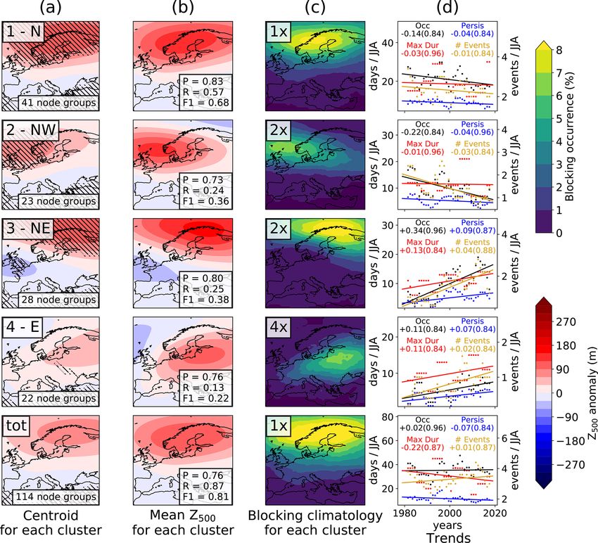
C. Thomas et al.: An unsupervised learning approach to identifying blocking events                                              585

the vertically averaged potential vorticity field (VPV), aver-      that the resulting blocking climatologies shown in Fig. A4
aged over 150–500 hPa. This approach was inspired by the            are broadly consistent with those presented in Fig. 6 of Pin-
work of Pelly and Hoskins (2003), who defined blocking as           heiro et al. (2019), underlining that this regional use of the
the negative latitudinal potential temperature gradient on the      BIs is still valid. Finally, to remove the well-known problem
dynamical tropopause. By taking a vertical average of the po-       of the AGP index identifying anomalous blocking events as-
tential vorticity field from the mid-troposphere to the lower       sociated with the subtropical high in summer (Davini et al.,
stratosphere, Schwierz et al. (2004) formulate a 3-D dynam-         2012), we adopt the extra threshold of the AGP index from
ically based index.                                                 Woollings et al. (2018). The subtropical high feature was not
   Another common approach to studying blocking trends is           observed in UKESM over Europe, since the zonal gradients
to use the absolute gradient of Z500 across fixed latitudes.        have a smaller magnitude, so the standard AGP index is used
This was first developed in Lejenäs and Økland (1983) and           for UKESM.
refined in a commonly applied form by Tibaldi and Molteni              We note that more indices have been proposed, includ-
(1990). This definition focuses on blocking events as persis-       ing hybrid approaches combining the AGP and DG83 in-
tent anticyclones that reverse the Z500 gradient. The method        dices (Barriopedro et al., 2010; Dunn-Sigouin et al., 2013;
has been adopted widely, refined (Diao et al., 2006; Barriope-      Woollings et al., 2018), the PV-θ approach developed by
dro et al., 2010) and extended to a range of latitudes (Scherrer    Pelly and Hoskins (2003) and the finite-amplitude wave ac-
et al., 2006).                                                      tivity (FAWA) method (Huang and Nakamura, 2015). K-
   All of these methods have been further developed by Pin-         means clustering analysis (Diday and Simon, 1980) has also
heiro et al. (2019), who applied four thresholds for each           been extensively used to study the Euro-Atlantic mid-latitude
blocking index: the magnitude of the anomaly, the persis-           variability and to identify weather regimes (Vautard, 1990;
tence of the blocking event (minimum 5 d), a minimum area           Michelangeli et al., 1995; Cassou, 2008; Ullmann et al.,
over which the anomaly takes place and an overlap criterion         2014; Strommen et al., 2019; Fabiano et al., 2021). How-
which measures if there is continuity across the blocked re-        ever, with the three BI methods included here in addition to
gion between different days (an overlap of the blocked con-         the SOM-BI and K-means clustering comparison in the case
tours). We adopt their thresholds and as such study the three       studies, we expect to see results that are sufficiently represen-
indices compared in Pinheiro et al. (2019) including their          tative of the range of blocking detection methods available
modifications:                                                      and to be able to highlight their most important similarities
                                                                    and discrepancies.
  – AGP – the geopotential height gradient method, which
    is the Tibaldi and Molteni (1990) index as adapted by
                                                                    2.4   Self-organizing map (SOM)
    Scherrer et al. (2006) to construct a two-dimensional
    field of geopotential height gradients;
                                                                    The fourth method we used to investigate trends in atmo-
  – DG83 – the Dole and Gordon (1983) method of investi-            spheric circulation regimes in European summer is self-
    gating positive geopotential height anomalies;                  organizing map cluster analysis (SOM; Kohonen, 1982).
                                                                    This is an increasingly popular unsupervised machine learn-
  – S04 – the Schwierz et al. (2004) method of identify-
                                                                    ing technique in synoptic meteorology to learn representative
    ing persistent anomalies in the potential vorticity field
                                                                    patterns of weather regimes and to investigate their trends
    (VPV) averaged over 150–500 hPa (VPV).
                                                                    (Hewitson and Crane, 2002; Liu and Weisberg, 2005; Huth
   We refer the reader to Sect. 2.2 in Pinheiro et al. (2019) for   et al., 2008; Sheridan and Lee, 2011; Johnson, 2013; Hor-
a detailed discussion of these methods and their associated         ton et al., 2015; Xu et al., 2016; Singh et al., 2016; Diff-
thresholds. However, our analysis differs from the method-          enbaugh et al., 2017; Sánchez-Benítez et al., 2019). In our
ology outlined by Pinheiro et al. (2019) in three ways, re-         context here, the SOM algorithm is trained with daily spatial
flecting the fact that our study is regional and seasonal in-       maps of dynamical states of the atmosphere above Europe,
stead of global. Firstly, we apply all thresholds defined by        as for example characterized by maps of geopotential height
Pinheiro et al. (2019) only to those grid cells within the re-      anomalies (Fig. 1b), potential vorticity (Fig. 1c) or sea level
gion of study so that we exclude events that are on the edges       pressure (Fig. A1b). By iteratively cycling through all sam-
of the domain. Such events would be considered blocking             ples of such meteorological maps, the algorithm learns rep-
events if the domain studied was extended. Secondly, Pin-           resentative patterns of atmospheric dynamical states, which
heiro et al. (2019) applied a spatial smoothing to their global     are referred to as “SOM nodes”.
threshold field, which defines the minimum threshold for               First, the number of nodes is specified and the SOM is
each grid cell to be blocked. Although we have applied the          initialized either with random values or with principal com-
LTDM smoothing of the seasonal cycle (which we subtract             ponent analysis patterns. Then for each day from the input
from variables to calculate field anomalies, Sect. 2.1) and we      field, the Euclidean distance between that daily meteorolog-
also use a spatially varying threshold field, we have not ap-       ical pattern and each node pattern is calculated. The node
plied this spatial smoothing to our threshold field. We found       with the smallest Euclidean distance to the sample day is

https://doi.org/10.5194/wcd-2-581-2021                                                Weather Clim. Dynam., 2, 581–608, 2021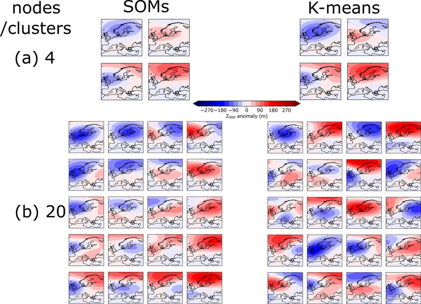
586                                     C. Thomas et al.: An unsupervised learning approach to identifying blocking events

Figure 2. The self-organizing map algorithm. Shown using a 3 × 3 node SOM with ERA5 Z500 JJA 1979–2019. The principal component
analysis (PCA)-initialized SOM pattern (step 1) has a much larger amplitude so it has been multiplied by 10−3 for visualization purposes.
The BMU refers to the best-matching unit, the SOM node which most closely matches the sample day.

known as the best-matching unit (BMU) for that day. Then               particular meteorological problem, is chosen by the user. In
the BMU pattern is updated to shift towards the pattern of             Sect. 3.3, we show how the SOM-BI performance depends
the sample day. The neighbouring SOM nodes (on the grid of             on the number of nodes and how this provides an objective
SOM nodes) are also updated to shift towards the sample day            criterion to select this number.
according to a Gaussian neighbourhood function. For each                  SOMs are of particular relevance in atmospheric science
cycle of iterations through all training samples, the updates          because they maintain the topological properties of the input
tend to become smaller as the SOM nodes converge towards               space. Once optimized, each node pattern represents a pos-
a representative pattern of atmospheric dynamical states. A            sible state of the atmosphere, and the nodes are arranged in
decay function on the updates is additionally applied, which           order of similarity, thus representing a continuum of atmo-
ensures convergence. Finally, a stable SOM is obtained with            spheric states. This contrasts with other methods of dimen-
a set of nodes that each provide a representative composite            sion reduction such as principal component analysis, where
of circulation patterns, arranged according to their similar-          the identified patterns are orthogonal. Such purely mathe-
ity on a row–column grid (i.e. the map). A diagram of the              matical representations are typically less meaningful from
training procedure is shown in Fig. 2. The number of nodes             a physical point of view, whilst each SOM node maintains
to be learned by the algorithm, or in other words the num-             physical significance as it can closely resemble actual atmo-
ber of representative weather patterns one aims to learn for a         spheric states found in meteorological data, with the nodes on

Weather Clim. Dynam., 2, 581–608, 2021                                                     https://doi.org/10.5194/wcd-2-581-2021
C. Thomas et al.: An unsupervised learning approach to identifying blocking events                                                           587

Figure 3. The SOM blocking index (SOM-BI). (a) The trained 3 × 3 SOM for the Z500 time-detrended anomaly. (b) Normalized histograms
showing the distributions of occurrence of BMUs for the days identified as blocked or non-blocked within the GTD. (c) The SOM-BI
optimization of the set of node groups against three different skill scores (precision (P ), recall (R) and F1 score) that are associated with the
GTD blocking events.

the row–column grid representing smooth transitions across                 Figure 3a shows the trained pattern for Z500 anomalies in
those possible atmospheric states (see the similarity of neigh-            ERA5 28 May–4 September 1979–2019 for nine nodes ar-
bouring nodes in the final SOM grid in Fig. 2). We have                    ranged in a 3 × 3 grid. Since each day in the dataset has been
implemented the SOM algorithm using the somoclu Python                     matched to a BMU, we can identify which nodes are asso-
package (Wittek et al., 2017).                                             ciated with blocked days according to our GTD. Figure 3b
   This property of SOMs is also the distinguishing feature                compares the histograms of those nodes which are and are
between SOMs and K-means clustering. In the case of K-                     not associated with the GTD blocking events. As expected,
means clustering, each node is updated at each iteration in-               the three nodes with large positive Z500 anomalies (nodes 1,
dependently and no neighbourhood function is applied. K-                   2 and 3) are most closely associated with blocking events,
means clustering tries to maximize differences between the                 and the nodes with large negative Z500 anomalies (nodes 7
centroids such that it does not learn a topology. This differ-             and 8) are rarely associated with blocking events. However,
ence between K-means clustering and SOMs is minor for                      nodes 1, 2 and 3 still occur on 15 % of non-blocked days, and
low node numbers, since the sharp differences in spatial pat-              28 % of the blocked days are also matched with one of the
terns are imposed on the SOMs and the neighbourhood func-                  other six nodes, including 3 % of blocked days matched with
tion has a limited effect. For larger node numbers, the SOM                nodes 7 and 8. This tells us that while the SOM nodes can
topology becomes smoother and the K-means centroids re-                    indicate the occurrence of blocked events, there is no node or
main distinct rather than representing a continuum of states,              single combination of nodes that can be consistently identi-
whereas a continuum is a more realistic reflection of the ac-              fied with blocking events with high skill.
tual atmosphere (Skific and Francis, 2012). A comparison be-                  However, from every 5 d period within the GTD, we can
tween SOMs and K-means analysis for 4 and 20 node/cluster                  identify an associated “group” of nodes. For example, a 5 d
numbers is shown in Fig. A5.                                               period can be associated with nodes 1 and 4 (any arrange-
                                                                           ment of nodes 1 and 4 across 5 d), and this would mean that
2.5   The self-organizing map blocking index (SOM-BI)                      [1, 4] is the associated group of nodes for that 5 d period.
                                                                           Since each 5 d period has been classified either as blocked or
Once we have created the GTD, this can be used to develop                  not blocked, it raises the possibility that a set of such groups
a new BI using SOM analysis. For a given variable from                     can be more specifically associated with blocking. We iden-
the ERA5 dataset, we can specify a node number and ar-                     tify the optimal set of node groups associated with blocking
rangement of nodes (number of rows and columns, Fig. 2)                    by ordering the list of all possible node groups (e.g. [1, 2, 3],
and then learn the corresponding SOM nodes from that data.

https://doi.org/10.5194/wcd-2-581-2021                                                         Weather Clim. Dynam., 2, 581–608, 2021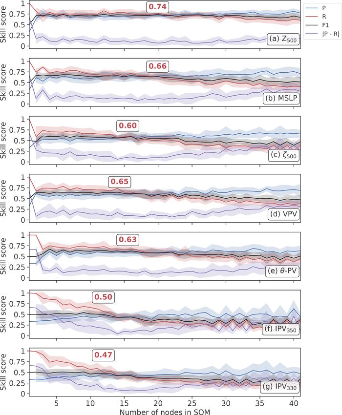
588                                     C. Thomas et al.: An unsupervised learning approach to identifying blocking events

[1, 4], [1], [1, 2, 3, 4, 6] etc.) from the node groups that have    2.7    SOM-BI application
the highest to lowest precision (P ) at identifying blocking
events.                                                              Once an optimal set of node groups has been identified, these
                                                                     can be used to classify days as blocked or not blocked. This
2.6   Classification skill measures                                  creates a time series of blocking events, but it does not pro-
                                                                     duce a spatial climatology. To develop a spatial climatology
Figure 3c shows the binary classification skill according to         for the SOM-BI, we use the BIs described in Sect. 2.3 across
the measures of precision, recall and F1 score when applying         the days that are identified as blocked by the SOM-BI.
the nine-node SOM-BI to ERA5 data. The three skill mea-                 A key advantage of the SOM-BI is that it identifies dis-
sures are shown for consecutive cases where we successively          tinct types of regional blocking events, since each blocked
add node groups as described above in order from highest to          node group within the set of node groups is associated with
lowest precision to the set of groups that we associate with         a set of blocking events. In the example shown in Fig. 3, 14
blocking. In other words, once a new group has been added            node groups are associated with blocking at the intersection
to the set of groups, this new group will define a series of         of precision and recall, which therefore identifies 14 possible
blocked periods within our SOM-BI approach. Precision (P )           distinct types of blocking. For example, the node group [1]
is defined as the ratio of true positives to total detected pos-     describes broad NW European events, [2] describes Scandi-
itives. For example, a precision of 0.8 indicates that 80 %          navian blocking, and [1, 2, 6] describes a more variable set
of the events identified by a method are true positives, and         of blocking patterns that are broadly associated with NE Eu-
the remaining 20 % of the events are false positives. Recall         rope.
(R) is the number of true positives divided by the total num-           To aid in our interpretation of these node groups, we cal-
ber of actual events. A recall of 0.8 indicates that 80 % of         culate the mean of their node codebooks, i.e. the mean of
all total blocking events are captured by the classification         the spatial patterns of the nodes in each node group, which
method, but 20 % of all total blocking events are false neg-         in turn also characterize the corresponding blocking patterns.
atives. A higher recall is typically associated with a loss in       This forms “mean codebooks” for each node group. Figure 4
precision, as identifying more events also means that one typ-       shows four examples of such node groups associated with
ically identifies more false positive events. Therefore, a care-     blocking from ERA5 Z500 for the case of 20 nodes – the
ful balance between precision and recall is usually sought           optimum number of nodes for this case (cf. Fig. 7a). These
after. One widely used skill metric to achieve this balance is       four node groups are chosen since they illustrate the vari-
the F1 score, which is the harmonic mean of precision and            ety of nodes and numbers of nodes present across the set of
recall:                                                              blocked node groups and also represent a variety of spatial
       2·P ·R                                                        patterns in blocking (N, NW, W and E). In Sect. 3.7, these
F1 =            ,                                              (1)
        P +R                                                         mean codebooks are applied to identify distinct categories of
which can vary between 0 (worst case, low detection skill)           blocking and to study their historical trends in ERA5.
and 1 (best score). If either P or R are low, the F1 score
tends towards 0, thus indicating low detection skill in at least
one of the two measures. For example, if there is a small            3     Results
number of node groups selected in the SOM-BI, the preci-
sion is very high but the recall is very low – a small num-          3.1    Case study analyses
ber of blocking events is well described but many blocking
events are missed by the classification. When a larger num-          We compare the blocking identification methods (i.e.
ber of node groups with a decreasing precision is included,          SOMs/SOM-BI, the three conventional BIs and K-means
then precision decreases and recall increases; more events are       clustering) for two examples of well-known 2003 and 2019
described but there is also a higher proportion of false posi-       European heat waves that were linked to blocking states of
tives. For the 3 × 3 SOM learned from ERA5 data, the node            the atmosphere (Figs. 5 and 6). In addition, we study two
group with the highest precision is [1], with P = 0.91 and           blocking events from UKESM to investigate how blocking
R = 0.15, followed by [2] with P = 0.89 and R = 0.19 and             events are described in the climate model. From the 101 years
[1, 2, 6] with P = 0.87 and R = 0.03. If only one node group         investigated in the pre-industrial control run we have found
is included in the set (e.g. [1] or [1, 2, 6]), there is a high P    the largest extent of heat extremes to occur in an extended
and low R, but as more node groups are added to the set of           heat wave shown in Appendix Fig. A2. This is contrasted
node groups (e.g. [1], [2]; then [1], [2], [1, 2, 6]), P decreases   with Fig. A3, which shows the end of a blocking event and a
but R increases. We identify the optimal set of node groups          weaker transitory anticyclone. Both UKESM events are dis-
by the value which maximizes the F1 score (Fig. 3c). We              cussed further in Appendix A.
perform this classification for a range of node numbers and             The 2003 European heat wave was a record-breaking heat
meteorological variables to identify an optimal performance          wave that had significant societal impacts (Robine et al.,
in Sect. 3.3.                                                        2008) and was shown to have been made at least twice

Weather Clim. Dynam., 2, 581–608, 2021                                                  https://doi.org/10.5194/wcd-2-581-2021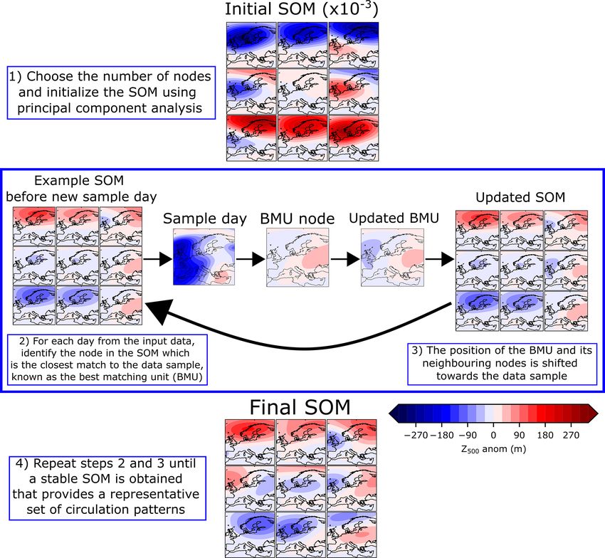
C. Thomas et al.: An unsupervised learning approach to identifying blocking events                                               589

Figure 4. Examples of four blocked node groups identified by the SOM-BI described in Sect. 2.5 averaged to form mean codebooks. Shown
here for Z500 in the optimized case of 20 nodes. There are 114 blocked node groups in total.

as likely due to anthropogenic climate change (Stott et al.,         perature extremes. Figures 5b and 6b show the vertically av-
2004). According to climate change projections, such heat            eraged potential vorticity (VPV) field, used by the S04 index
waves will become commonplace by the 2040s irrespec-                 to identify blocking, and also the 10 m winds. The VPV field
tive of future emissions scenarios (Christidis et al., 2014).        is consistently anti-correlated with the Z500 field and signif-
The most extreme temperatures during this heat wave were             icant negative anomalies in the VPV field tend to be asso-
recorded from the 6–12 August, where the peak tempera-               ciated with stationary surface winds, particularly across 26–
ture recorded was in Southern France at 41 ◦ C. Black et al.         29 June 2019. Figures 5c and 6c show the BMU SOM pattern
(2004) report that atmospheric flow anomalies were recorded          for the case of nine nodes for detrended Z500 anomaly fields.
in early August, although there was a relatively weak signa-         Whilst the SOM nodes clearly track the features shown in the
ture of blocking. The 2003 heat wave remained the Euro-              Z500 maps, a range of BMUs are identified in both case stud-
pean temperature record until 2019, when surface temper-             ies even though there is a consistent extreme weather event
atures of 46 ◦ C were observed in central France. The 2019           across these time periods. In the 2003 case study in ERA5,
heat wave was concurrent with persistent hot air that origi-         three SOM BMUs and four transitions between BMUs are
nated in North Africa (the so-called “Saharan heat bubble”),         shown in Fig. 5c. These all show positive Z500 anomalies in
which was sustained by an omega block centred on western             the northern part of the domain, even though the meteoro-
Europe (Mitchell et al., 2019).                                      logical situation varies meridionally more than zonally, par-
   Figures 5a and 6a show daily maps of detrended Z500               ticularly across 4–9 August 2003. An even greater variety of
anomalies for the two events, the field used by the DG83             BMUs is observed in the 2019 case, where four nodes and
index to identify blocking events. The hatching indicates de-        four transitions between SOM nodes are shown in Fig. 6c.
trended surface temperature extremes at the 90th and 99th               This creates a difficulty of interpretation – whilst the SOM
percentile. It can be seen that across all cases there are signif-   can identify the best-matching spatial pattern of Z500 anoma-
icant positive Z500 anomalies which are associated with tem-         lies, these particular SOM patterns do not correspond to cir-

https://doi.org/10.5194/wcd-2-581-2021                                                 Weather Clim. Dynam., 2, 581–608, 2021
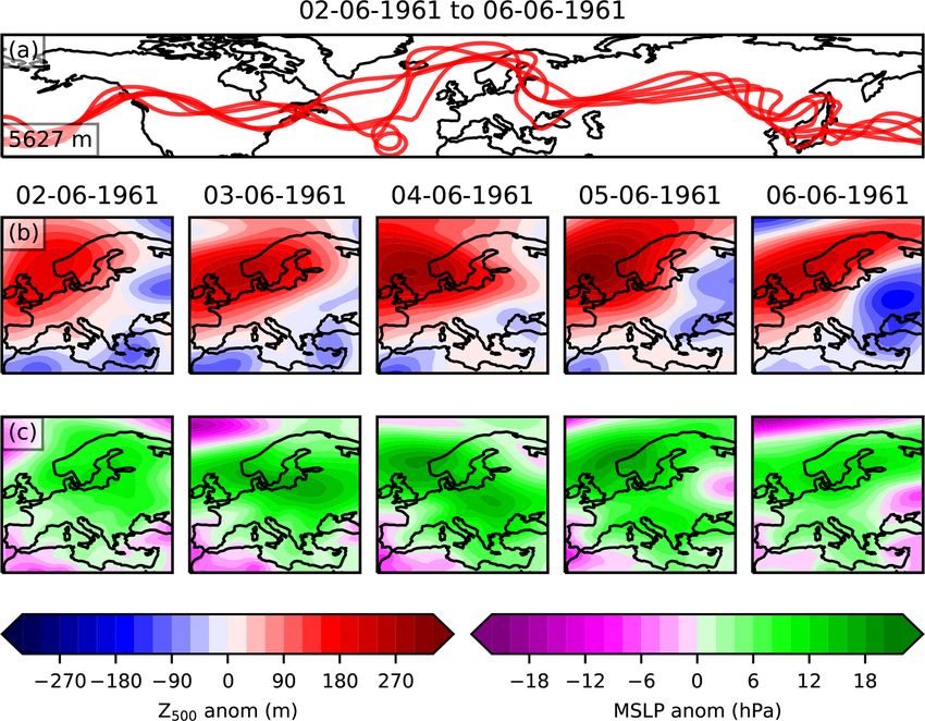
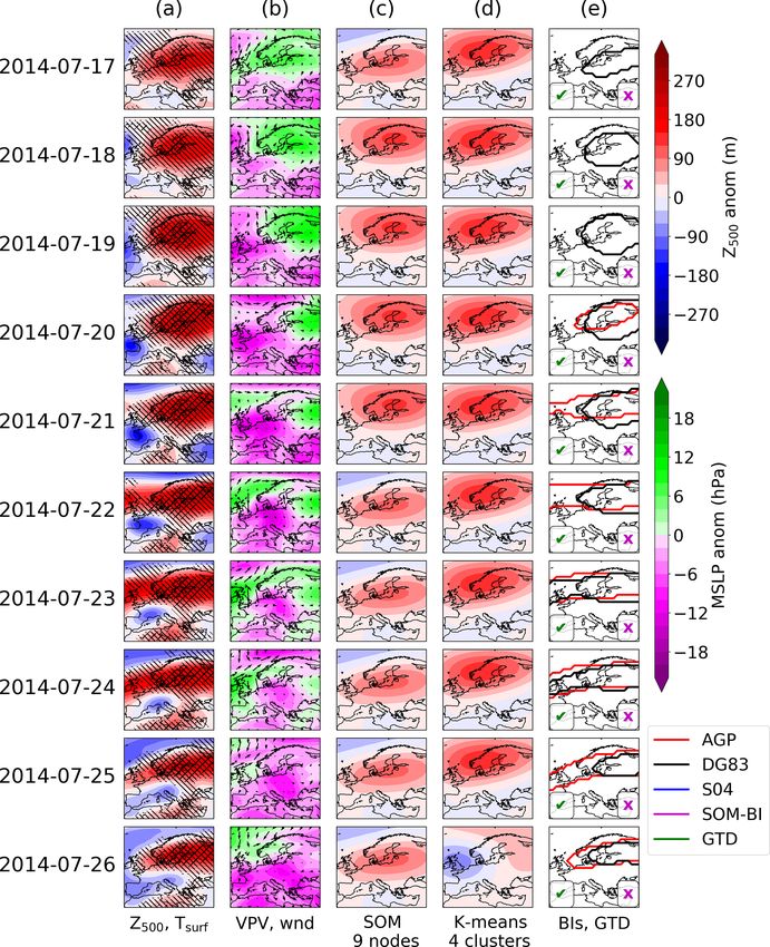
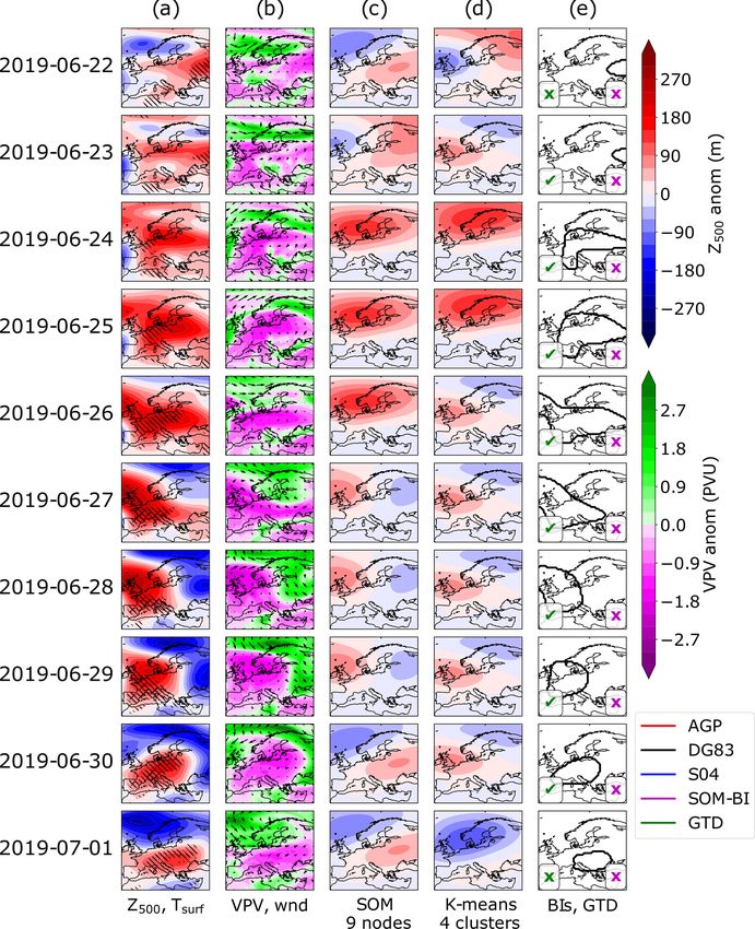
590                                     C. Thomas et al.: An unsupervised learning approach to identifying blocking events

Figure 5. The 2003 European heat wave. Column (a) shows the detrended 500 hPa geopotential height anomaly for each day. Left (right)
hatching indicates where the local surface temperature exceeds the 90th (99th) percentile for the detrended 2 m temperature. Column (b)
shows the potential vorticity anomaly vertically averaged across 150–500 hPa, with arrows showing the 10 m wind field. Column (c) shows
the corresponding SOM pattern for Z500 anomalies from nine nodes. Column (d) similarly shows the corresponding K-means centroid for
four clusters. Column (e) shows the contours identified as blocked in this region in the AGP (red), DG83 (black) and S04 (blue) indices. A
green (magenta) tick or cross indicates if the GTD (SOM-BI) identifies the day as blocked or not.

culation regimes as conventionally understood, since even              the Mediterranean), the SOMs become less distinguishable
minor shifts in the domain (such as the change from the                and lose even more of their explanatory power to represent
2–3 August 2003) can cause the corresponding pattern to                meaningful pattern variations across the domain (not shown).
shift. The frequency of these shifts and sensitivity of the            Overall, the fact that several SOM nodes occur during the
SOM is dependent on both the number of nodes chosen and                case study blocking events shows that individual SOM pat-
the domain size. Smaller domains with fewer SOMs show                  terns will not be able to consistently identify blocking events
more consistency in the synoptic weather patterns, but when            with high precision or recall, contrary to how SOMs are typ-
these are sufficiently reduced (such as for four SOMs over             ically used in many applications in the literature. However,

Weather Clim. Dynam., 2, 581–608, 2021                                                      https://doi.org/10.5194/wcd-2-581-2021
C. Thomas et al.: An unsupervised learning approach to identifying blocking events                                        591

Figure 6. As in Fig. 5 but for the 2019 European heat wave.

well-defined groups of nodes, as we will show below, can in-   on 31 July to the UK on 8 August 2003 is not described
deed achieve this task and can thus be used for the purpose    by four centroids. For the 2019 heat wave in Fig. 6d, all
of our new SOM-BI.                                             four weather regimes are represented, and the blocked pe-
   Figures 5d and 6d show a K-means clustering analysis us-    riod is primarily associated with a mixed weather regime.
ing Z500 anomaly fields for the case of four centroids. As     This shows that the 2019 case is also not described well by
described in Sect. 2.4, the case of K-means clustering with    K-means clustering.
four centroids produces a similar set of weather regimes to       Figures 5e and 6e show the contours denoting blocked re-
SOMs with four nodes. Consequently, the K-means analysis       gions as identified by the three different BIs. A tick or cross
exhibits a similar behaviour to the SOMs discussed above but   in the bottom left and right corners indicates whether the day
distinguishing between fewer weather regimes. One weather      was identified as blocked or not in the GTD or the SOM-BI.
regime indicating Scandinavian blocking consistently repre-    For the SOM-BI labelling, Z500 20 SOM nodes are chosen
sents the 2003 European heat wave across Fig. 5d, but the      on the basis of the optimization of the SOM-BI in Fig. 7a.
westward shift of the high-pressure centre from Scandinavia    Across all case studies the DG83 index clearly tracks regions

https://doi.org/10.5194/wcd-2-581-2021                                          Weather Clim. Dynam., 2, 581–608, 2021
592                                     C. Thomas et al.: An unsupervised learning approach to identifying blocking events

Figure 7. A comparison of the performance of the SOM blocking index for seven variables in the ERA5 1979–2019 historical period with a
varying number of nodes in the SOM. Precision (P ), recall (R) and F1 scores are calculated, and the absolute difference between precision
and recall is also shown. Error bands show the standard deviation (±1σ ) for 10-fold cross-validation. The red number inset into each panel
shows the optimal F1 score, and the position of the box indicates the corresponding optimal node number. The optimal value is defined by
the node number where the F1 score is close to its maximum value and the difference between precision and recall is close to the minimum
value.

of positive Z500 anomalies. The S04 and AGP indices also                27–30 June 2019 indicate mixed patterns which do not ob-
track the same feature in the 2003 heat wave until 3 August             viously correspond to blocking over a consistent area (the
2003 but do not identify any blocking associated with the               positive maxima shift from the British Isles to eastern Eu-
2019 heat wave. The SOM-BI describes the initial period of              rope within a day). This lack of pattern consistency is mostly
the 2003 heat wave well, although it does not capture the               the result of an unfortunate balance between the positive and
western European blocking event during the peak period of               negative Z500 anomalies on these days, where the latter play
extreme temperature across 6–12 August. The SOM-BI also                 a major role in the allocation of the BMU during this pe-
does not capture the 2019 blocking pattern coincident with              riod. We discuss the possibility of ignoring negative anoma-
the 2019 heat wave. This is because the SOM nodes are too               lies in our assignments of the BMUs in Sect. 3.6 but found
variable over the 2019 event such that the set of nodes which           that this modification does not improve the SOM-BI perfor-
best match the Z500 anomaly fields are not generally asso-              mance overall. In summary, there are blocking events such as
ciated with blocking. For example, the SOM nodes across                 these that will also not be described well by the new SOM-

Weather Clim. Dynam., 2, 581–608, 2021                                                       https://doi.org/10.5194/wcd-2-581-2021
C. Thomas et al.: An unsupervised learning approach to identifying blocking events                                                   593

Table 1. A comparison of skill scores of the original BIs and the new SOM-BI against the GTD for ERA5 1979–2018 and UKESM for JJA
over the European domain. Where not indicated the skill scores are measured with respect to the relevant GTD. “BLO” indicates the skill
score for the trivial case of every day labelled as blocked and “RND” where a random allocation of blocked days has occurred with the same
proportion of blocked days as the GTD.

   Dataset    Method      Days blocked     Precision    Recall      F1    F1 wrt AGP    F1 wrt DG83     F1 wrt S04     F1 wrt SOM-BI
   ERA5       GTD                33.4 %            1         1      1            0.56            0.73          0.19               0.74
   ERA5       AGP                19.5 %         0.76      0.44   0.56               1            0.55          0.22               0.51
   ERA5       DG83               34.3 %         0.72      0.75   0.73            0.55               1          0.19               0.69
   ERA5       S04                 5.3 %         0.69      0.11   0.19            0.22            0.19             1               0.15
   ERA5       SOM-BI             34.6 %         0.73      0.75   0.74            0.51            0.69          0.15                  1
   ERA5       BLO                 100 %         0.33         1   0.50            0.33            0.51          0.10               0.51
   ERA5       RND                33.4 %         0.33      0.33   0.33            0.25            0.34          0.09               0.34
   UKESM      GTD                29.0 %            1         1      1            0.34            0.60             –               0.71
   UKESM      AGP                20.8 %         0.41      0.29   0.34               1            0.29             –               0.28
   UKESM      DG83               14.5 %         0.90      0.45   0.60            0.29               1             –               0.55
   UKESM      SOM-BI             29.6 %         0.70      0.72   0.71            0.28            0.55             –                  1
   UKESM      BLO                 100 %         0.29         1   0.45            0.34            0.25             –               0.46
   UKESM      RND                29.0 %         0.29      0.29   0.29            0.24            0.19             –               0.29

BI, but as we show below the SOM-BI performs as good as                  ERA5 and UKESM, the best blocking index is the SOM-BI,
or even better than many conventional BIs in most cases.                 with a F1 score of 0.74 in ERA5 and 0.71 in UKESM. All
                                                                         of the indices consistently perform worse in UKESM than
3.2   Blocking index comparison in ERA5 and UKESM                        in ERA5. This is because blocking is less frequent in the
      with GTD                                                           model, and several of those blocking patterns identified in
                                                                         UKESM are less distinct (Fig. A3). This is probably asso-
A climatological comparison of the BIs over JJA Europe                   ciated with mean biases in the representation of Z500 that
confirms what has been discussed in the case study analy-                have been observed across several climate models (Scaife
ses above and is consistent with the results of Pinheiro et al.          et al., 2010; Schaller et al., 2018). The DG83 index performs
(2019), which are broadly consistent with other BI clima-                almost as well as the SOM-BI in ERA5 with an F1 score
tologies. We show the spatial distribution of blocking clima-            of 0.73, but there is a significant reduction in performance
tologies according to three conventional blocking indices in             to 0.60 when applied to UKESM data. The AGP index in
Fig. A4. Where our analysis substantially differs from the lit-          turn shows an even weaker skill than DG83 in both reanaly-
erature is in our regional approach and consideration of direct          sis and model, with a larger drop in skill from 0.56 to 0.34
time series comparisons among the BIs as well as to our new              in ERA5 and UKESM, respectively. The fact that SOM-BI
SOM-BI. We do not explicitly consider the time-averaged                  still shows a relatively good score for UKESM of 0.71 sug-
climatological distributions of blocking events over Europe              gests that the SOM-BI can be particularly useful in studying
(as shown in Fig. A4). For our comparison, we first apply all            regional blocking in climate models. In particular, since a
BIs to the historical ERA5 data over the European domain.                model ensemble may exhibit a variety of intensities of block-
Each day for each BI is labelled as blocked if a blocking                ing, the SOM-BI would be able to overcome the limitations
event has been identified within the European sector and per-            of BIs, where (particularly in the case of AGP) thresholds
sists for at least 5 d. A blocking event is not identified if the        are defined with respect to the observational record. Since
thresholds for amplitude, persistence, area and overlap dis-             the anomalous flow patterns associated with blocking will
cussed in Sect. 2.3 are not met within the European domain.              be more consistent across datasets, the SOM-BI can identify
This results in a binary dataset for each BI that identifies pe-         blocking events across a model ensemble with greater accu-
riods of at least 5 consecutive days where blocking patterns             racy. The consistent skill of the SOM-BI across both ERA5
exist within the European sector. We then compare these bi-              and UKESM has been further verified by swapping the train-
nary BI datasets to our manually labelled GTD.                           ing and test datasets between each dataset, as described in
   Table 1 compares the precision, recall and F1 scores of               Sect. 3.5.
these BIs and our new SOM-BI against the GTD for this                       A case where every day in Europe is labelled as blocked
domain-based comparison in both ERA5 and UKESM. We                       (“BLO”) is also compared, which represents the case of per-
further compare the time series of blocking classifications              fect recall (= 1) but a low precision. This case gives an
among the BIs themselves to quantify how consistent the BIs              F1 score of 0.53 for the GTD for ERA5 and 0.45 for the
are with each other. The key results are underlined. In both             GTD of UKESM and provides a useful benchmark of ba-

https://doi.org/10.5194/wcd-2-581-2021                                                    Weather Clim. Dynam., 2, 581–608, 2021
594 C. Thomas et al.: An unsupervised learning approach to identifying blocking events
sic performance. Surprisingly, the AGP index only performs
marginally better than BLO for ERA5 and performs worse in
the UKESM case. Whilst S04 has a higher precision than
BLO, because the recall is so low the total F1 score is
much lower (0.19). Finally, we compare a random labelling
of blocked and non-blocked days, where the proportion of
blocked days is equal to that of the GTD (“RND”). This gives
an equal precision and recall because the number of true pos-
itives is equal to the number of false negatives. The F1 score
of RND still exceeds that of S04, with 0.33 for ERA5 and
0.29 for UKESM, and is comparable to the F1 score of AGP
in UKESM.
3.3 SOM-BI skill dependence on the choice of SOM
node number and the meteorological variable
The key hyperparameter in the SOM-BI is the number of
nodes (k), which here is similar to identifying the optimal
number of circulation patterns required to effectively clas-
sify European summer weather regimes. In addition, there Figure 8. A comparison of the SOM blocking index performance
for three variables in 101 years from the UKESM pre-industrial
are a number of meteorological variables from which we
control period with a varying number of nodes in the SOM. Pre-
could learn the SOM patterns, which in turn will also in-
cision (P ), recall (R) and F1 scores are calculated, and the absolute
fluence the skill of our SOM-BI method. The dependency difference between precision and recall is also shown. Error bands
of the skill of our BI on these two factors is quantified in show the standard deviation (±1σ ). The red number inset into each
the following. Figures 7 and 8 show how precision (P ), re- panel shows the optimal F1 score, and the position of the box in-
call (R) and F1 score depend on k and the meteorological dicates the corresponding node number. As above, the largest F1
variable in ERA5 and UKESM, respectively. Specifically, we score is for Z500 , indicating that Z500 is the best variable tested for
compare the skill metrics for cases where we learn the SOM analysing blocking patterns using the SOM-BI in UKESM.
nodes from Z500 , MSLP and ζ500 anomalies. For ERA5, we
additionally consider four PV-related variables (VPV, θ -PV,
IPV350 and IPV330 ) shown in Fig. 7d–g.
Another hyperparameter related to the number of nodes is
the row x column (n × m) arrangement of nodes. For exam-
ple, 16 nodes can be arranged as 16×1, 4×4, 8×2, 2×8 or
1 × 16. These different arrangements affect the topology of
the SOM, the initialization of the nodes and which nodes are
counted in the neighbourhood of other nodes during the up-
date process of the SOM (Fig. 2). For each k in Figs. 7–9 we
have used the arrangement of nodes that maximizes the av-
erage number of nearest neighbours between each node (e.g.
using 4 × 4 nodes for k = 16). This approach maximally ex- Figure 9. The number of node groups that are identified as blocked
ploits the SOM topology. We have also used n>m (for exam- in the SOM-BI for ERA5 and UKESM for a range of node numbers
ple using a 9 × 2 arrangement instead of a 2 × 9 arrangement and variables. The panels separate the variables available in both
of nodes for k = 18) to preferentially arrange the SOM topol- models from those only available in ERA5. Error bands show the
ogy zonally across the domain rather than meridionally. This standard deviation (±1σ ).
is done because there is greater variability in the occurrence
of blocking patterns zonally than meridionally across Europe
(Fig. A4). This ensures that the SOM-BI has not been tuned to the data
The results are shown for 1 ≤ k ≤ 41. To measure out- we measure our skill against, which could give it an unfair
of-sample skill, we used 10-fold cross-validation, where the advantage compared to the other BIs. For ERA5 we used
GTD was split into 10 separate sections for testing the SOM- 4-year periods (1980–1984,. . . , 2015–2019 inclusive) to test
BI. The SOM-BI is trained on 9 of the 10 data sections, and on and trained on the remaining 37 years, with each 4-year
its skill is evaluated on the remaining section. The skill scores period once serving as the independent test set. In UKESM
shown only indicate how well the SOM-BI is able to predict 10-year periods (1960–1959,. . . , 2050–2059 inclusive) were
the test period in question, which was not used for training. used for testing the SOM-BI, and it was trained on the re-
Weather Clim. Dynam., 2, 581–608, 2021 https://doi.org/10.5194/wcd-2-581-2021C. Thomas et al.: An unsupervised learning approach to identifying blocking events 595
maining 91-year period. This 10-fold cross-validation proce- test data to ensure that the skill evaluation is truly indepen-
dure produces a range of precision, recall and F1 scores for dent, following the idea of statistical cross-validation (see
each node number. Figures 7 and 8 show the mean values for e.g. Nowack et al., 2018; Mansfield et al., 2020). Figure 10
precision, recall, F1 and the absolute difference between pre- shows the results of this analysis for Z500 and 20 nodes
cision and recall. Figure 9 compares the number of groups across both (a) ERA5 and (b) UKESM datasets, which is the
of nodes identified as blocked for each variable. Error bands best-performing case according to our analysis above. Since
indicate the standard deviation of each skill metric (±1σ ). the datasets have different lengths (41 years vs. 101 years),
Common features are observed for each variable for a very we tested the model on 4 and 10 years for each dataset re-
small or large number of SOM nodes. For small k the SOM- spectively. For a small number of years, the algorithm only
BI identifies more days as blocked, such that R
P . This sees a few blocking events and so only identifies the par-
indicates that the SOM is under-fitting the data for European ticular node groups that are associated with these blocking
circulation patterns across the domain, and so the algorithm events rather than identifying node groups that are in general
lacks a precise delineation of blocking events. In other words, associated with blocking events. This leads to a high preci-
it could be beneficial to increase k to be able to represent sion for a small number of training years, particularly in the
a larger number of dynamical states and thus to detect and ERA5 data, since the SOM-BI is effectively overfitting on a
describe blocking events more precisely. For large k, R
P , few events, but the recall and overall F1 score are low. This
showing that the SOM-BI is trending towards overfitting the behaviour is confirmed by Fig. 10c, which shows that there
training data. We deduce that the optimal k occurs when the is a small set of node groups associated with blocking for a
difference between P and R is small and the F1 score is close small number of training years.
to its maximum value. Figure 10a and b both show that the recall and F1 scores
From Figs. 7 and 8 we find that for both ERA5 and increase asymptotically for a larger number of training years,
UKESM the Z500 anomaly is the best variable to use with the and the precision decreases asymptotically. These varia-
SOM-BI, with a mean F1 score of 0.74 and 0.71 for k = 20 tions become very small after 20 years for both ERA5 and
and 21 in ERA5 and UKESM respectively. From Fig. 9a, UKESM, which indicates that for around 20 years the SOM-
Z500 also shows the lowest number of blocked node groups BI seems to have achieved an optimal performance. Figure 9c
for a given k, which shows that the blocked node groups are shows that the number of node groups associated with block-
physically more explanatory in Z500 than the blocked node ing continues to increase in both ERA5 and UKESM even
groups associated with other variables, making the SOM- after this point, with 120 node groups identified with block-
BI results easier to interpret physically. MSLP is the second ing for UKESM over 91 years compared to 95 node groups
most effective variable, with an optimum F1 score of 0.66 over 37 years. However, these extra node groups occur rarely
and 0.64 for ERA5 and UKESM respectively. This lower in the blocking datasets since they do not significantly affect
peak performance is because the MSLP field has a lower either the precision or recall of the algorithm and are there-
signal-to-noise ratio as it is influenced by effects within the fore not physically meaningful.
boundary layer such as heat lows. The PV-related variables
exhibit a variety of lower skills, where the VPV field per- 3.5 Cross-comparison of SOM-BI skill
forms at a similar level to MSLP, since the vertical integra-
tion of the VPV variable enables it to capture the pattern For the SOM-BI to be effectively applied to understand fu-
of blocking better than other PV-based variables (Schwierz ture trends in atmospheric blocking, we need to verify that
et al., 2004). the training of the SOM-BI on the observational record is
consistent with CMIP6 models. This step is necessary to en-
3.4 SOM-BI skill dependence on number of training sure that the SOM-BI can identify blocking patterns in the
years models. If it is possible for the SOM-BI to identify block-
ing patterns in a CMIP6 model from training on the obser-
One important verification for the SOM-BI is to ensure its vations, then this shows potential for the SOM-BI to be ap-
robustness over long timescales. Contrary to the other BIs, plied consistently across a model ensemble. Furthermore, if
the SOMs learn from training data. Therefore, the SOM-BI the SOM-BI can be trained on a CMIP6 model and tested
skill on test data will also be a function of how representative on the observations, differences in the skill of the SOM-BI
the training samples are of general states of the atmosphere. would highlight limitations in that model’s ability to repre-
Here we investigate if the observational record, for exam- sent blocking patterns. This could be applied across a model
ple, is long enough to indeed ensure the same performance ensemble to compare the skill of different models at repre-
of the SOM-BI described above over longer timescales. For senting blocking patterns.
this purpose, we train the SOM-BI algorithm on a range of To investigate the feasibility of such studies, we test the
different numbers of training years, while keeping the num- skill of the SOM-BI algorithm by training Z500 data on the
ber of years to test the algorithm performance consistent. 41 years from the ERA5 dataset and testing on the UKESM
Importantly, there is no overlap between the training and and vice versa. Table 2 shows the differences in the opti-
https://doi.org/10.5194/wcd-2-581-2021 Weather Clim. Dynam., 2, 581–608, 2021You can also read