Drivers of diffusive CH4 emissions from shallow subarctic lakes on daily to multi-year timescales
←
→
Page content transcription
If your browser does not render page correctly, please read the page content below
Biogeosciences, 17, 1911–1932, 2020
https://doi.org/10.5194/bg-17-1911-2020
© Author(s) 2020. This work is distributed under
the Creative Commons Attribution 4.0 License.

Drivers of diffusive CH4 emissions from shallow subarctic lakes on
daily to multi-year timescales
Joachim Jansen1,2,z , Brett F. Thornton1,2 , Alicia Cortés3 , Jo Snöälv4 , Martin Wik1,2 , Sally MacIntyre3 , and
Patrick M. Crill1,2
1 Department  of Geological Sciences, Stockholm University, Stockholm, Sweden
2 Bolin Centre for Climate Research, Stockholm, Sweden
3 Marine Science Institute, University of California at Santa Barbara, Santa Barbara, USA
4 Department of Geography, University of Exeter, Exeter, UK
z Invited contribution by Joachim Jansen, recipient of the EGU Biogeosciences Outstanding

Student Poster and PICO Award 2017.

Correspondence: Joachim Jansen (joachim.jansen@geo.su.se)

Received: 15 August 2019 – Discussion started: 23 August 2019
Revised: 2 March 2020 – Accepted: 6 March 2020 – Published: 8 April 2020

Abstract. Lakes and reservoirs contribute to regional car-        supply to the water column. Spectral analysis indicated that
bon budgets via significant emissions of climate forcing trace    on timescales shorter than a month, emissions were driven
gases. Here, for improved modelling, we use 8 years of float-     by wind shear whereas on longer timescales variations in wa-
ing chamber measurements from three small, shallow subarc-        ter temperature governed the flux. Long-term monitoring ef-
tic lakes (2010–2017, n = 1306) to separate the contribution      forts are essential to identify distinct functional relations that
of physical and biogeochemical processes to the turbulence-       govern flux variability on timescales of weather and climate
driven, diffusion-limited flux of methane (CH4 ) on daily to      change.
multi-year timescales. Correlative data include surface wa-
ter concentration measurements (2009–2017, n = 606), total
water column storage (2010–2017, n = 237), and in situ me-
teorological observations. We used the last to compute near-      1   Introduction
surface turbulence based on similarity scaling and then ap-
                                                                  Inland waters are an important source of the radiatively ac-
plied the surface renewal model to compute gas transfer ve-
                                                                  tive trace gas methane (CH4 ) to the atmosphere (Bastviken
locities. Chamber fluxes averaged 6.9±0.3 mg CH4 m−2 d−1
                                                                  et al., 2011; Cole et al., 2007). On regional to global scales,
and gas transfer velocities (k600 ) averaged 4.0 ± 0.1 cm h−1 .
                                                                  an estimated 21 %–46 % of ice-free season CH4 emissions
Chamber-derived gas transfer velocities tracked the power-
                                                                  from lakes, ponds, and reservoirs occur via turbulence-driven
law wind speed relation of the model. Coefficients for the
                                                                  diffusion-limited gas exchange (Bastviken et al., 2011; Del-
model and dissipation rates depended on shear production
                                                                  Sontro et al., 2018; Wik et al., 2016b) (hereafter abbrevi-
of turbulence, atmospheric stability, and exposure to wind.
                                                                  ated to “diffusive fluxes”). Diffusive fluxes are often mea-
Fluxes increased with wind speed until daily average val-
                                                                  sured with floating chambers (Bastviken et al., 2004), but
ues exceeded 6.5 m s−1 , at which point emissions were sup-
                                                                  gas transfer models are increasingly used, for example in
pressed due to rapid water column degassing reducing the
                                                                  regional emission budgets (Holgerson and Raymond, 2016;
water–air concentration gradient. Arrhenius-type tempera-
                                                                  Weyhenmeyer et al., 2015). Fluxes computed with modelled
ture functions of the CH4 flux (Ea0 = 0.90 ± 0.14 eV) were
                                                                  gas transfer velocities agree to a certain extent with floating
robust (R 2 ≥ 0.93, p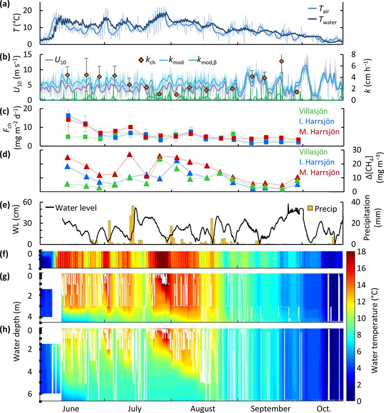
1912                                                                     J. Jansen et al.: Drivers of diffusive CH4 emissions

parisons are needed to identify weather- and climate-related         CH4 emissions to the atmosphere also depend on the rates
controls on the flux that are appropriate for seasonal assess-    of methane metabolism regulated by substrate availability
ments. Considering the increased use of process-based ap-         and temperature-dependent shifts in enzyme activity and mi-
proaches in regional emission estimates (Tan and Zhuang,          crobial community structure (Borrel et al., 2011; McCalley et
2015), understanding the mechanisms that drive the compo-         al., 2014; Tveit et al., 2015). Arrhenius-type relationships of
nents of the diffusive flux is imperative for improving emis-     CH4 fluxes have emerged from field studies (DelSontro et al.,
sion estimates.                                                   2018; Natchimuthu et al., 2016; Wik et al., 2014) and across
                                                                  latitudes and aquatic ecosystem types in synthesis reports
Drivers of diffusive CH4 emissions                                (Rasilo et al., 2015; Yvon-Durocher et al., 2014). However,
                                                                  the temperature sensitivity is modulated by biogeochemical
Diffusive fluxes at the air–water interface are estimated with    factors that differ between lake ecosystems, such as nutri-
a two-layer model (Liss and Slater, 1974):                        ent content (Davidson et al., 2018; Sepulveda-Jauregui et
                                                                 al., 2015), methanotrophic activity (Duc et al., 2010; Lofton
F = k Caq − Cair,eq .                                      (1)    et al., 2014), predominant emission pathway (DelSontro et
                                                                  al., 2016; Jansen et al., 2019), and warming history (Yvon-
   The flux F (mg CH4 m−2 d−1 , hereafter abbreviated             Durocher et al., 2017). In lakes, the air–water concentration
mg m−2 d−1 ) depends on the concentration difference across       difference driving the flux (Eq. 1) is further affected by fac-
a thin layer immediately below the air–water interface            tors that dissociate production from emission rates. These in-
(1[CH4 ], mg m−3 ), of which the upper boundary is in equi-       clude biotic factors, such as aerobic and anaerobic methan-
librium with the atmosphere (Cair,eq ) and the base represents    otrophy, and abiotic factors such as hydrologic inputs of ter-
the bulk liquid (Caq ) and is limited by the gas transfer ve-     restrially produced CH4 (Miettinen et al., 2015; Paytan et al.,
locity k (m d−1 ). k has been conceptualized as characterizing    2015) and storage-and-release cycles associated with tran-
transfer across the diffusive boundary layer. Other models        sient stratification (Czikowsky et al., 2018; Jammet et al.,
envision exchange as driven by parcels of water intermit-         2017; Vachon et al., 2019). Given these interacting functional
tently in contact with the atmosphere. In these surface re-       dependencies, the magnitude of fluxes has complex patterns
newal models, k depends on the frequency of the renewal           of temporal variability.
events (Csanady, 2001; Lamont and Scott, 1970). The result-          Disentangling the physical and biogeochemical drivers of
ing calculation for k is based on the Kolmogorov velocity         the diffusive CH4 flux remains a challenge. The component
scale uη = (εν)1/4 , where ε is dissipation rate of turbulent     drivers respond differently to slow and fast changes in mete-
kinetic energy (TKE) and ν is kinematic viscosity (Tennekes       orological covariates (Baldocchi et al., 2001; Koebsch et al.,
and Lumley, 1972). Progress has been made in understand-          2015) such that different mechanisms may explain the diel
ing how to compute ε and gas transfer rates as a function         and seasonal variability of the flux. For example, tempera-
of wind speed and the heating and cooling at the lake’s sur-      ture affects emissions through convective mixing on short
face (Tedford et al., 2014). Comparisons between models and       timescales and through the rate of sediment methanogene-
other flux estimation methods, such as the eddy covariance        sis on longer timescales; the diurnal cycle of insolation may
technique, illustrate the improved accuracy when computing        have a limited effect on production because the heat capacity
gas transfer velocities using turbulence-based as opposed to      of the water buffers the temperature signal (Fang and Stefan,
wind-based models (Czikowsky et al., 2018; Heiskanen et           1996). Similar phase lags and amplifications may lead to hys-
al., 2014; Mammarella et al., 2015).                              teretic flux patterns, such as cold season emission peaks due
   The supply of sparingly soluble trace gases to the air–        to release of gases from the hypolimnion in dimictic lakes
water interface moderates fluxes when concentrations are          (Encinas Fernández et al., 2014; López Bellido et al., 2009)
higher within the water column than in the atmosphere. Trace      or thermal inertia of lake sediments (Zimov et al., 1997).
gases such as CH4 are produced in the sediments and diffuse       Spectral analysis of the flux and its components can improve
into the overlying water. During stratification, these gases      our understanding of the flux variability by quantifying how
may accumulate if the density gradient restricts the efficacy     much power is associated with key periodicities (Baldocchi
of wind mixing. Thermal convection associated with surface        et al., 2001).
cooling can deepen the mixed layer and transfer stored gas to        Here we present a high-resolution, long-term dataset
the surface, enhancing emissions (Crill et al., 1988; Eugster     (2010–2017) of diffusive CH4 fluxes from three subarctic
et al., 2003). Temporal patterns of stratification and mixing     lakes estimated with floating chambers (n = 1306) and fluxes
contribute to variability in diffusive CH4 fluxes (López Bel-     obtained by modelling using in situ meteorological observa-
lido et al., 2009; Podgrajsek et al., 2016) and concentrations    tions and surface water concentrations (n = 535). The sur-
(Loken et al., 2019; Natchimuthu et al., 2016). Periodic emis-    face renewal model is used to compute gas transfer veloci-
sions from storage at depth have been particularly difficult to   ties. Arrhenius relationships of 1[CH4 ] and fluxes of CH4
resolve in lake emission budgets (Bastviken et al., 2004; Wik     are also calculated. Using spectral analysis of our time series
et al., 2016b).                                                   data, we distinguish the temporal dependency of abiotic and

Biogeosciences, 17, 1911–1932, 2020                                                   www.biogeosciences.net/17/1911/2020/
J. Jansen et al.: Drivers of diffusive CH4 emissions                                                                      1913

biotic controls on the flux. The effects of lake size and wind   turbulent processes such as convection, we compared fluxes
exposure are illustrated by comparing results from the three     from shielded and unshielded chambers on days when the
different lakes.                                                 lake mean bubble flux was < 1 % of the lake mean diffusive
                                                                 flux (bubble traps, 2009–2017; Jansen et al., 2019; Wik et al.,
                                                                 2013). Averaged over the three lakes, the difference was sta-
2     Materials and methods                                      tistically significant (0.20 ± 0.16 mg m−2 d−1 , n = 58, mean
                                                                 ±95 % CI), but small in relative terms (6 % of the mean flux).
2.1    Field site
                                                                 Conversely, some types of floating chambers can enhance
CH4 emissions were measured from three subarctic lakes           gas transfer by creating artificial turbulence when dragging
of postglacial origin (Kokfelt et al., 2010), located around     through the water (Matthews et al., 2003; Vachon et al., 2010;
the Stordalen Mire in northern Sweden (68◦ 210 N, 19◦ 020 E,     Wang et al., 2015). Ribas-Ribas et al. (2018), Banko-Kubis
Fig. 1), a palsa mire complex underlain by discontinuous per-    et al. (2019), and Gålfalk et al. (2013) assessed gas trans-
mafrost (Malmer et al., 2005). The Mire (350 m a.s.l.) is part   fer velocities in floating chambers of similar design, size,
of a catchment that connects Mt. Vuoskoåiveh (920 m a.s.l.)      and flotation depth as those used in this study. Ribas-Ribas
in the south to Lake Torneträsk (341 m a.s.l.) in the north      et al. (2018) and Banko-Kubis et al. (2019) measured TKE
(Lundin et al., 2016; Olefeldt and Roulet, 2012). Villasjön      dissipation rates with acoustic Doppler velocimetry (ADV)
is the largest and shallowest of the lakes (0.17 km2 , 1.3 m     inside and outside the chamber perimeter and concluded that
max. depth) and drains through fens into a stream feeding        the chambers did not cause artificial turbulence. Gålfalk et
Mellersta Harrsjön and Inre Harrsjön, which are 0.011 and        al. (2013) similarly found good agreement between k600 de-
0.022 km2 in size and have maximum depths of 6.7 m and           rived from free-floating chamber observations with a CH4
5.2 m, respectively (Wik et al., 2011). The lakes are normally   tracer and k600 computed independently from nearby ADV
ice-free from the beginning of May through the end of Octo-      measurements and an infrared (IR) imaging technique.
ber. Manual observations were generally conducted between
mid-June and the end of September. Diffusion accounts for        2.3   Water samples
17 %, 52 %, and 34 % of the ice-free CH4 flux in Villasjön,
Inre, and Mellersta Harrsjön, respectively, with the remain-     Surface water samples were collected 0.2–0.4 m below the
der emitted via ebullition (2010–2017; Jansen et al., 2019).     surface at two to three different locations in each lake, at
                                                                 1- to 2-week intervals from June to October (Fig. 1). Sam-
2.2    Floating chambers                                         ples were collected from the shore with a 4 m Tygon tube
                                                                 attached to a float to avoid disturbing the sediments (2009–
We used floating chambers to directly measure the                2014) and from a rowboat over the deepest points of Inre
turbulence-driven diffusive CH4 flux across the air–water        and Mellersta Harrsjön (2010–2017) and at shallows (< 1 m
interface (Fig. 1). They consisted of plastic tubs covered       water depth) on either end of the lakes (2015–2017) using
with aluminium tape to reflect incoming radiation and were       a 1.2 mL × 3.2 mm i.d. Tygon tube. In addition, water sam-
equipped with polyurethane floats and flexible sampling          ples were collected at the deepest point of Inre and Meller-
tubes capped at one end with three-way stopcocks (Bastviken      sta Harrsjön at 1 m intervals down to 0.1 m from the sedi-
et al., 2004). Depending on flotation depth, each chamber        ment surface with a 7.5 mL × 6.4 mm i.d. fluorinated ethy-
covered an area between 610 and 660 cm2 and contained            lene propylene (FEP) tube. Subsequently, 60 mL polypropy-
a headspace of 4 to 5 L. Chambers were deployed in pairs         lene syringes were rinsed thrice with sample water before du-
with a plastic shield mounted 30 cm below one chamber of         plicate bubble-free samples were collected and were capped
each pair to deflect methane bubbles rising from the sedi-       with airtight three-way stopcocks. The 30 mL samples were
ment. Every 1–2 weeks during the ice-free seasons of 2010        equilibrated with 30 mL headspace and shaken vigorously by
to 2017, two to four chamber pairs were deployed in Vil-         hand for 2 min (2009–2014) or on a mechanical shaker at
lasjön and four to seven chamber pairs were deployed in Inre     300 rpm for 10 min (2015–2017). Prior to 2015, outside air –
and Mellersta Harrsjön in different depth zones (Fig. 1). The    with a measured CH4 content – was used as headspace. From
number of chambers and deployment intervals exceeded the         2015 on we used an N2 5.0 headspace (Air Liquide). Water
minimum needed to resolve the spatio-temporal variability of     sample conductivity was measured over the ice-free season
the flux (Wik et al., 2016a). Over a 24 h period, two to four    of 2017 (n = 323) (S230, Mettler-Toledo) and converted to
60 mL headspace samples were collected from each chamber         specific conductance using a temperature-based approach.
using polypropylene syringes, and the flotation depth and air
temperature were noted in order to calculate the headspace       2.4   Concentration measurements
volume. The 24 h deployment period integrates diel varia-
tions in the gas transfer velocity (Bastviken et al., 2004).     Gas samples were analysed within 24 h after collection at
   The fluxes reported here are from the shielded chambers       the Abisko Scientific Research Station, 10 km from the
only. To check that the shields were not reducing fluxes from    Stordalen Mire. Sample CH4 contents were measured on a

www.biogeosciences.net/17/1911/2020/                                                    Biogeosciences, 17, 1911–1932, 2020
1914                                                                        J. Jansen et al.: Drivers of diffusive CH4 emissions

Figure 1. Map of the Stordalen Mire field site (a). Chamber and sampling locations are shown as they were in 2015–2017. A schematic of
the floating chamber pairs is shown in (b). Lake bathymetry from Wik et al. (2011). Satellite imagery: ©Google, DigitalGlobe, 2017.

Shimadzu GC-2014 gas chromatograph which was equipped                and Millero, 1977), using lake-averaged specific conductiv-
with a flame ionization detector (GC–FID) and a 2.0 m long,          ity and a salinity factor (mS cm−1 ) × (g kg−1 )−1 of 0.57. The
3 mm i.d. stainless-steel column packed with 80/100 mesh             salinity factor was based on a linear regression of simul-
HayeSep Q and used N2 > 5.0 as a carrier gas (Air Liquide).          taneous measurements of conductivity and dissolved solids
For calibration we used standards of 2.059 ppm CH4 in N2             (R 2 = 0.99, n = 7) in five lakes in the Torneträsk catchment
(Air Liquide). A total of 10 standard measurements were              (Miljödata-MVM, 2017). We defined the depth of the surface
made before and after each run. After removing the highest           mixing layer (zmix ) at a density gradient threshold (dρ / dz)
and lowest values, relative standard deviations of the stan-         of 0.03 kg m−3 m−1 (Rueda et al., 2007).
dard runs were generally less than 0.25 %.
                                                                     2.6   Meteorology
2.5    Water temperature, pressure, density, and
       mixed-layer depth                                             Meteorological data were collected from four different masts
                                                                     on the Mire and collectively covered a period from June 2009
Water temperature was measured every 15 min from 2009                to October 2018 with half-hourly measurements of wind
to 2018 with temperature loggers (HOBO Water Temp Pro                speed, air temperature, relative humidity, air pressure, and
v2, Onset Computer) in Villasjön and at the deepest loca-            irradiance (Fig. 1, Table 1). Wind speed was measured with
tions within Inre and Mellersta Harrsjön. Sensors were de-           3D sonic anemometers at the Palsa tower (z = 2.0 m), the
ployed at 0.1, 0.3, 0.5, and 1.0 m depth in all lakes, with          Villasjön shore tower (z = 2.9 m), the InterAct Lake tower
additional sensors at 3.0, 5.0 m (IH and MH), and 6.7 m              (z = 2.0 m), and the Integrated Carbon Observation Sys-
(MH). Sensors were intercalibrated prior to deployment in            tem (ICOS) site (z = 4.0 m). Air temperature and relative
a well-mixed water tank and by comparing readouts just be-           humidity were measured at the Palsa tower, at the Vil-
fore and during the onset of freezing when the water col-            lasjön shore tower (Rotronic MP100a (2012–2015)/Vaisala
umn was isothermal. In this way a precision of < 0.05 ◦ C was        HMP155 (2015–2017)), and at the InterAct lake tower. In-
achieved. The bottom sensors were buried in the surface sed-         coming and outgoing shortwave and long-wave radiation
iment and were excluded from in situ intercalibration. Water         were monitored with net radiometers at the Palsa tower (Kipp
pressure was measured in Mellersta Harrsjön (5.5 m) with             & Zonen CNR1) and at the InterAct lake tower (Kipp & Zo-
a HOBO U20 water level logger (Onset Computer). Water                nen CNR4). Precipitation data were collected with a Weath-
density was computed from temperature and salinity (Chen             erHawk 500 at the ICOS site. Overlapping measurements

Biogeosciences, 17, 1911–1932, 2020                                                       www.biogeosciences.net/17/1911/2020/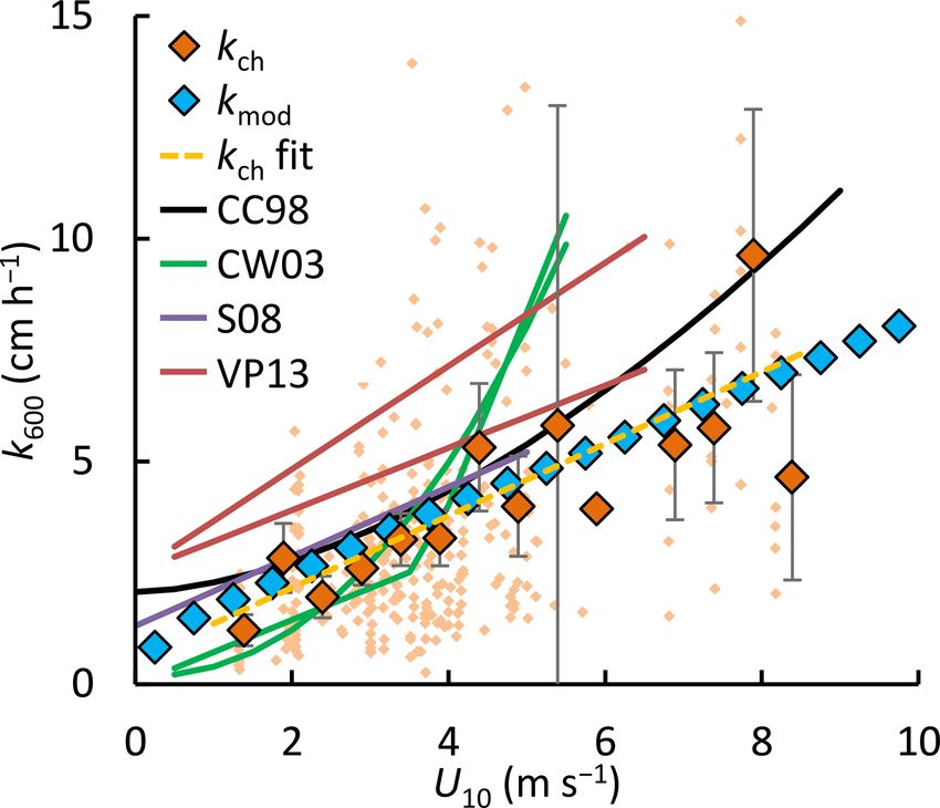
J. Jansen et al.: Drivers of diffusive CH4 emissions                                                                            1915

were cross-validated and averaged to form a single time se-
ries.

2.7   Computation of CH4 storage and residence time

The amount of CH4 stored in the water column (g CH4 m−2 )
was computed by weighting and then adding each concen-
tration measurement by the volume of the 1 m depth inter-
val within which it was collected. For the upper 2 m of the
two deeper lakes, we separately computed storage in the veg-
etated littoral zone from nearshore concentration measure-
ments, as these values could be different from those further
from shore due to outgassing and oxidation during horizontal
transport (DelSontro et al., 2017). We computed the average
residence time of CH4 in the lake by dividing the amount
stored by the lake mean surface flux. Residence times com-
puted with this approach should be considered upper lim-          Figure 2. Example of chamber headspace CH4 concentrations ver-
its, because in this calculation we assumed that removal pro-     sus deployment time. Measured concentrations (dots) are averages
cesses other than surface emissions, such as microbial oxi-       from 2015 to 2017 (0.1 h) and 2011 (1–24 h); error bars repre-
dation, were negligible or took place at the sediment–water       sent the 95 % confidence intervals. Linear regressions (dashed black
                                                                  lines) show the rate increase over 1 h (two measurements) and over
interface with minimal effect on water column CH4 .
                                                                  24 h (five measurements). The solid red line represents chamber
2.8   Flux calculations                                           concentrations computed with Eq. (2). The rate increase associated
                                                                  with the mean 24 h flux corrected for headspace accumulation is
In order to calculate the chamber flux with Eq. (1), we es-       shown as a dashed red line (Eq. 1 with kch from Eq. 2, or Eq. 3 with
                                                                  c1 = 1.21). Labels denote fluxes calculated from the linear regres-
timated the gas transfer velocity, kch (cm h−1 ), from the
                                                                  sion slopes (Eq. 3, black) and from Eq. (2) (red).
time-dependent equilibrium chamber headspace concentra-
tion Ch,eq (t) (mg m−3 ) (Bastviken et al., 2004):
                                      KH RTwater A k t              Figure 2 shows that the headspace correction is necessary
 Caq − Ch,eq (t) = Caq − Ch,eq (t0 ) e−

                                              V      ch , (2)     to avoid underestimating fluxes. The headspace-corrected
where KH is Henry’s law constant for CH4 (mg m−3 Pa−1 )           flux (dashed red line) equals the initial slope of Eq. (2) (solid
(Wiesenburg and Guinasso, 1979), R is the universal gas con-      red line) and is about 21 % higher than the non-corrected flux
stant (m3 Pa mg−1 K−1 ), Twater is the surface water tempera-     (lower dashed black line in Fig. 2). However, both Eq. (2)
ture (K), and V and A are the chamber volume (m3 ) and            (solid red line) and Eq. (3) with c1 = 1 (dashed black lines) fit
area (m2 ), respectively. This method accounts for gas accu-      the concentration data (R 2 ≥ 0.98 for 94 % of 24 h flux mea-
mulation in the chamber headspace, which reduces the con-         surements). This similarity results partly because the fluxes
centration gradient and limits the flux (Eq. 1) (Fig. 2). For a   were low enough to keep headspace concentrations well be-
subset of chamber measurements where simultaneous water           low equilibrium with the water column. Short-term mea-
concentration measurements were unavailable (n = 949) we          surements (upper dashed black line) may omit the need for
computed the flux from the headspace concentrations alone:        headspace correction (Bastviken et al., 2004). Because con-
           ∂xh PV                                                 centration measurements were not available for all chamber
F = c1 M               .                                    (3)   observations, we used multi-year mean values of 1[CH4 ]
            ∂t RTair A
                                                                  and kch to compute c1 as a function of chamber deployment
∂xh /∂t is the headspace CH4 mole fraction change                 time. For 24 h chamber deployments, c1 = 1.21.
(mol mol−1 d−1 ) computed with ordinary least-squares
(OLS) linear regression (Fig. 2), M is the molar mass of          2.9   Computing gas transfer velocities with the surface
CH4 (0.016 mg mol−1 ), P is the air pressure (Pa), and Tair             renewal model
is the air temperature (K). Scalar c1 corrects for the accu-
mulation of CH4 gas in the chamber headspace and increases        We used the surface renewal model (Lamont and Scott, 1970)
over the deployment time. Comparing both chamber flux cal-        formulated for small eddies at Reynolds numbers > 500
culation methods, we find c1 = 1.21 for 24 h deployments          (MacIntyre et al., 1995; Theofanous et al., 1976) to estimate
(OLS, R 2 = 0.85, n = 357). Chambers were sampled up to           k:
four times during their 24 h deployment (at 10 min, 1–5 h,                       1      1
                                                                  kmod = α(εν) 4 Sc− 2 ,                                          (4)
and 24 h), which allowed us to compute fluxes at time inter-
vals of 1 and 24 h. P and Tair were averaged over the relevant    where the hydrodynamic and thermodynamic forces driving
time interval.                                                    gas transfer are expressed, respectively, as the TKE dissipa-

www.biogeosciences.net/17/1911/2020/                                                        Biogeosciences, 17, 1911–1932, 2020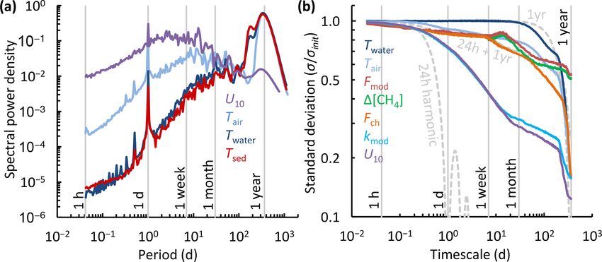
1916                                                                              J. Jansen et al.: Drivers of diffusive CH4 emissions

Table 1. Location and instrumentation of meteorological observations on the Stordalen Mire, 2009–2018.

 Identifier    Period         Location              Wind                       Air temp. and humidity    Radiation       Reference
 Palsa tower   2009–2011      68◦ 210 19.6800 N     C-SAT 3                    HMP-45C                   CNR-1           Olefeldt et al. (2012)
                              19◦ 20 52.4400 E      Campbell Scientific        Campbell Scientific       Kipp & Zonen
 Villasjön     2012–2018      68◦ 210 14.5800 N     R3-50                      MP100a, Rotronic          REBS Q7.1       Jammet et al. (2015)
 shore tower                  19◦ 30 1.0700 E       Gill                       HMP155, Vaisala           Campbell Sci.
 InterAct      2012–2018      68◦ 210 16.2200 N     uSonic-3 Scientific        CS215                     CNR-4           –
 Lake tower                   19◦ 30 14.9800 E      Metek                      Campbell Scientific       Kipp & Zonen
 ICOS site     2013–2018      68◦ 210 20.5900 N                              WeatherHawk 500                             –
                              19◦ 20 42.0800 E                               Campbell Scientific

tion rate ε (m2 s−3 ) and the dimensionless Schmidt number
Sc, defined as the ratio of the kinematic viscosity v (m2 s−1 )
to the free solution diffusion coefficient D0 (m2 s−1 ) (Jähne
et al., 1987; Wanninkhof, 2014). The scaling parameter α
has a theoretical value of 0.37 (Katul et al., 2018) but
is often estimated empirically (α 0 ) to calibrate the model
(e.g. Wang et al., 2015). To allow for a qualitative com-
parison between model and chamber fluxes, we took ratios
                                      1     1
of kch (floating chambers) and (εν) 4 Sc− 2 (surface renewal
model, half-hourly values of kmod averaged over each cham-
ber deployment period) and determined α 0 = 0.23 ± 0.02 for
all lakes (mean ±95 % CI, n = 334) (Fig. 3), α 0 = 0.31 ±
0.06 (n = 67) for Villasjön, α 0 = 0.25 ± 0.03 (n = 136) for
Inre Harrsjön, and α 0 = 0.17 ± 0.02 (n = 131) for Meller-
sta Harrsjön (Supplement Fig. S1). Calibrating the model
in this way allowed us to assess whether chamber flux rela-
                                                                          Figure 3. Determination of the model scaling parameter α 0 via
tionships with wind speed and temperature were reproduced
                                                                          comparison between gas transfer velocities from floating cham-
by the model. For similar comparative purposes, k values                  bers (Eq. 2) and the surface renewal model (Eq. 4 with α 0 = 1 and
were normalized to a Schmidt number of 600 (CO2 at 20 ◦ C)                Sc = 600, half-hourly values averaged over each chamber’s 24 h
(Wanninkhof, 1992): k600 = (600/Sc)−0.5 k. The wind speed                 deployment period) for all three lakes. Dots represent individual
at 10 m (U10 ) was computed from measured wind speed fol-                 chamber deployments (grey) and multi-chamber means for each
lowing Smith (1988), assuming a neutral atmosphere.                       weekly deployment in 2016 and 2017, when concentration mea-
   We used a parametrization by Tedford et al. (2014) based               surements were taken simultaneously with, and in close proximity
on Monin–Obukhov similarity theory to estimate the TKE                    to, the chamber measurements (black). Mean ratios, and therefore
dissipation rate at half-hourly time intervals:                           α 0 , are represented by the slopes of the dotted lines. Error bars rep-
                                                                          resent 95 % confidence intervals of the means.
        0.56u3∗w /κz + 0.77β if β > 0 (cooling)

ε=                                                          (5)
        0.6u3∗w /κz              if β ≤ 0 (heating),
                                                                          (J kg−1 K−1 ) is the water specific heat, and ρw (kg m−3 )
where u∗w is the water friction velocity (m s−1 ), κ is the               is the water density. Qeff (W m−2 ) represents the net heat
von Kármán constant, and z is depth below the water sur-                  flux into the mixing layer and is the sum of net short-
face (0.15 m, the depth for which Eq. 5 was calibrated). We               wave and long-wave radiation and sensible and latent heat
determined u∗w from the air friction velocity u∗a assum-                  fluxes. Penetration of radiation into the water column was
ing equal shear stresses (τ ) on both sides of the air–water              evaluated across seven wavelength bands via Beer’s law
interface, τ = ρa u2∗a = ρw u2∗w , and taking into account at-            (Jellison and Melack, 1993). An attenuation coefficient of
mospheric stability (MacIntyre et al., 2014; Tedford et al.,              0.74 was computed for the visible portion of the spec-
2014). β is the buoyancy flux (m2 s−3 ), which accounts for               trum from Secchi depth (2.3 m; Karlsson et al., 2010) fol-
turbulence generated by convection (Imberger, 1985):                      lowing Idso and Gilbert (1974). Net long-wave radiation
β = αT gQeff /cpw ρw .                                         (6)        (LWnet = LWout − LWin ) was computed via measurements of
                                                                          LWin (Table 1) and LWout = σ T 4 , where σ is the Stefan–
  Here, αT is the thermal expansion coefficient (m3 K−1 )                 Boltzmann constant (5.67 × 10⁻⁸ W m−2 K−4 ) and T is the
(Kell, 1975), g is the standard gravity (m s−2 ), cpw                     surface water temperature in kelvin. LWnet time series were

Biogeosciences, 17, 1911–1932, 2020                                                                  www.biogeosciences.net/17/1911/2020/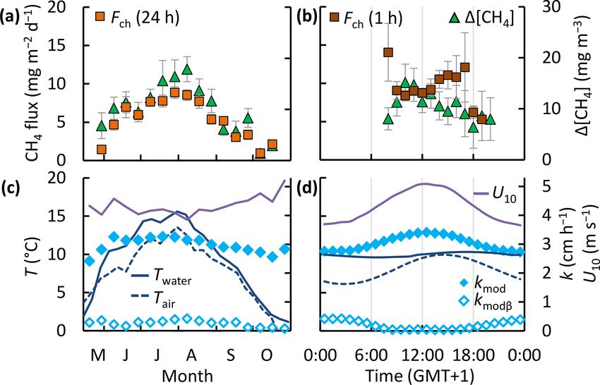
J. Jansen et al.: Drivers of diffusive CH4 emissions                                                                        1917

gap-filled with ice-free mean values for each lake. Sensible      1989). Data gaps were filled by linear interpolation. We re-
and latent heat fluxes were computed with the bulk aerody-        moved the linear trend from the original time series to reduce
namic formula (MacIntyre et al., 2002). Both Qeff and β are       red noise, and we block-averaged spectra (eight segments
here defined as positive when the heat flux is directed out of    with 50 % overlap) to suppress aliasing at higher frequen-
the water, for example when the surface water cools.              cies. We normalized the spectral densities by multiplying by
   Direct measurements of ε in an Arctic pond (1 m depth,         the frequency and dividing by the variance of the original
0.005 km2 surface area) demonstrate that Eq. (5) can charac-      time series (Baldocchi et al., 2001).
terize near-surface turbulence in small, sheltered water bod-        We evaluated our discontinuous (fluxes, concentrations)
ies similar to the lakes studied here (MacIntyre et al., 2018).   and continuous (meteorology) time series with a cli-
When the near surface was strongly√stratified at instrument       macogram, an intuitive way to visualize a continuum of vari-
depth (buoyancy frequencies (N = g/ρw × dρw /dz) > 25             ability (Dimitriadis and Koutsoyiannis, 2015). It displays
cycles per hour, cph), the required assumption of homoge-         the change of the standard deviation (σ ) with averaging
neous isotropic turbulence was not met and Eq. (5) could not      timescale (tavg ). Variables were normalized by lake to cre-
be evaluated. We observed cases with N >25 cph < 3 % of the       ate a single time series at half-hourly resolution (e.g. 48
time.                                                             entries for each 24 h chamber flux). To compute each stan-
                                                                  dard deviation (σ (tavg )) data were binned according to aver-
2.10   Calculation of binned means                                aging timescale, which ranged from 30 min to 1 year. Be-
                                                                  cause of the discontinuous nature of the datasets, n bins
We binned data to assess correlations between the flux and        were distributed randomly across the time series. We chose
environmental covariates. Half-hourly values of water tem-        n = 100 000 to ensure that the 95 % confidence interval of
perature and wind speed were averaged over the deployment         the standard deviation at the smallest bin size was less than
period of each chamber (fluxes) and over 24 h prior to the        1 % of the value of σ (Sheskin, 2007). To allow for compar-
collection of each water sample (concentrations), reflecting      ison between variables, we normalized each σ series by its
the mean residence time of CH4 in the water column. Fluxes,       initial smallest-bin value: σnorm = σ/σinit . For timescales < 1
concentrations, and k values were then binned in 10 d, 1 ◦ C,     week we used 1 h chamber observations, noting that sparse
and 0.5 m s−1 bins to obtain relationships with time, water       daytime-only observations of concentrations and 1 h fluxes
temperature, and wind speed, respectively. The 10 d bins typ-     may underestimate short-term variability (σinit ). We use the
ically contained at least 1 sampling day for each overlap-        climacogram to test whether the variability of the diffusive
ping year and enabled representative averaging across years.      CH4 flux is contained within meteorological variability, as
Lake-dependent variables (e.g. flux) were normalized by lake      for terrestrial ecosystem processes (Pappas et al., 2017).
to obtain a single time series (divided by the lake mean, mul-
tiplied by the overall mean).                                     2.13   Statistics

2.11   Calculation of the empirical activation energy             We used analysis of variance (ANOVA) and the t test to com-
                                                                  pare means of different groups. The use of means, rather than
Chamber and modelled fluxes as well as concentrations were        medians, was necessary because annual emissions can be de-
fitted to an Arrhenius-type temperature function (e.g. Wik et     termined by rare high-magnitude emission events. Paramet-
al., 2014; Yvon-Durocher et al., 2014):                           ric tests were justified because of the large number of sam-
          0                                                       ples in each analysis, in accordance with the central limit the-
F = e−Ea /kB T +b ,                                        (7)    orem. Linear regressions were performed with the ordinary
                                                                  least-squares method (OLS): reported p values refer to the
where kB is the Boltzmann constant (8.62 × 10⁻⁵ eV K−1 )          significance of the regression slope. Non-linear regressions
and T is the water temperature in kelvin. The em-                 were optimized with the Levenberg–Marquardt algorithm for
pirical activation energy (Ea 0 , in electron volts (eV),         non-linear least squares with confidence intervals based on
1 eV = 96 kJ mol−1 ) was computed with a linear regression        bootstrap replicates (n = 1999). Computations were carried
of the natural logarithm of the fluxes and concentrations onto    out in MATLAB 2018a and in PAST v3.25 (Paleontological
the inverse temperature (K−1 ), of which b is the intercept.      Statistics software package) (Hammer et al., 2001).
2.12   Timescale analysis: power spectra and
       climacogram

We computed power spectra for near-continuous time series
of the surface sediment, water and air temperature, and wind
speed according to Welch’s method (pwelch in MATLAB
2018a), which splits the signal into overlapping sections and
applies a cosine tapering window to each section (Hamming,

www.biogeosciences.net/17/1911/2020/                                                     Biogeosciences, 17, 1911–1932, 2020
1918 J. Jansen et al.: Drivers of diffusive CH4 emissions
3 Results layer depth and water temperature in the deeper lakes, along
with wind speed, air temperature, and precipitation for the
3.1 Measurements and models ice-free period of 2017. The ice-free period consisted of
two phases. In the first, air and surface water temperatures
Chamber fluxes averaged 6.9 mg m−2 d−1 (range 0.2–32.2, were higher and the two deeper lakes were stratified. Wind
n = 1306) and closely tracked the temporal evolution of the speeds increased to mean values approaching 5 m s−1 for a
surface water concentrations (mean 11.9 mg m−3 , range 0.3– few days at a time and then decreased for a day or two. Deep
120.8, n = 606), with the higher values in each lake mea- mixing events followed surface cooling and heavy rainfall.
sured in the warmest months (July and August, Fig. 4a, e). Water level maxima and surface temperature minima were
Diffusive fluxes increased with wind speed and water tem- observed 2–3 d after rainfall events, for example between
perature (Fig. 4b,c). Reduced emissions were measured in 15 and 18 July 2017 (Fig. 5e). In the second phase, wind
the shoulder months (June and September) and were associ- speeds were persistently higher (U10 >5 m s−1 ), air and sur-
ated with lower water temperatures. We also observed abrupt face water temperatures declined, and all lakes were mixed
reductions of the flux at wind speeds lower than 2 m s−1 to the bottom. Strong nocturnal cooling on 16 August 2017
and higher than 6.5 m s−1 . Surface water concentrations gen- broke up stratification and the lakes remained well-mixed un-
erally increased with temperature and peaked in the sum- til ice formation (20 October). Throughout the ice-free sea-
mer months, but unlike the chamber fluxes they decreased sons from 2009 to 2018, stratified periods (zmix ≤ 1 m) lasted
with increasing wind speed (Fig. 4f, g). Relationships with for 7 h on average and were common (31 % and 45 % of the
wind speed were approximately linear, while relationships time in Inre and Mellersta Harrsjön, respectively), but were
with temperature fitted an Arrhenius-type exponential func- frequently disrupted by deeper mixing events. Shallow mix-
tion (Eq. 7). Activation energies were not significantly dif- ing (zmix ≤ zmean ) occurred on diel timescales. Deeper mix-
ferent when using either surface water or sediment tempera- ing occurred at longer intervals (days to weeks) and more
ture (Ea0 = 0.90 ± 0.14 eV, R 2 = 0.93 and Ea0 = 1.00 ± 0.17, frequently toward the end of the ice-free season (Fig. 5g, h)
R 2 = 0.93, respectively, mean ±95 % CI). The fluxes, con- in association with higher wind speeds.
centrations, and wind speed were non-normally distributed Fluxes and near-surface concentrations also varied within
(Fig. 4d, h, o). Surface water temperatures (0.1–0.5 m) were these periods. CH4 concentrations and fluxes were higher in
normally distributed around the mean of each individual the warmer, stratified period and lower in the colder, mixed
month of the ice-free season (Fig. 4n), but the composite dis- periods. In 2017, the highest concentrations and fluxes oc-
tribution was bimodal. curred earlier in the season, with the initial high values in
Fluxes computed with the surface renewal model (Eq. 1 the two deeper lakes indicative of residual CH4 that had
using kmod ) closely resembled the chamber fluxes (Eq. 3) in not escaped to the atmosphere immediately after ice melt,
terms of temporal evolution (Fig. 4a) and correlation with around 1 June 2017 (Fig. 5c, d). As residual CH4 was emit-
environmental drivers (Fig. 4b, c). Mean model fluxes were ted, near-surface concentrations declined and then in the first
slightly higher than the chamber fluxes in Villasjön and Inre half of the stratified period (July 2017, Fig. 5d), particularly
Harrsjön and slightly lower in Mellersta Harrsjön (Table 2). in Mellersta Harrsjön, increased with increased rainfall and
Model fluxes were significantly different between littoral and with temperature. During this period, kch and kmod were sim-
pelagic zones in Inre and Mellersta Harrsjön (paired t tests, ilar. Decreases in kch were coupled to increases in thermal
p ≤ 0.02), reflecting spatial differences in the surface wa- energy input via two mechanisms: (1) when the air tempera-
ter concentration (Table 2). Similar to the chamber fluxes, ture increased above the surface water temperature in the day,
the air–water concentration difference (1[CH4 ]) explained leading to a stable atmosphere over the lakes, and (2) when
most of the temporal variability of the modelled emissions; the near-surface temperature was warmer and the water col-
both kmod (Eq. 4) and kch (Eq. 2) were functions of U10 umn was stratified to the surface. Thus, lower fluxes occurred
(Fig. 4k) and did not display a distinctive seasonal pattern during the second part of the stratified period (August 2017,
(Fig. 4i). Modelled fluxes decreased at higher wind speeds Fig. 5c) when surface concentrations increased during warm-
when surface concentrations decreased and displayed a cut- ing periods when winds were light, the atmosphere was sta-
off at daily mean U10 ≥ 6.5 m s−1 , similar to the chamber ble during the day, and the upper water column was strongly
fluxes, but not at U10J. Jansen et al.: Drivers of diffusive CH4 emissions 1919
Table 2. CH4 fluxes from floating chambers and the surface renewal model as well as surface CH4 concentrations. Data from 2014 were
excluded from the model flux means because of a substantial bias in the timing of sample collection. Model fluxes for each lake were
computed with lake-specific scaling parameter values (Fig. S1).
Chamber flux (mg m−2 d−1 ) Modelled flux (mg m−2 d−1 ) Surface concentration (mg m−3 )
Location Mean ±95 % CI n Mean ±95 % CI n Mean ±95 % CI n
Overall 6.9 ± 0.3 1306 7.6 ± 0.5 501 11.9 ± 0.9 606
Villasjön 5.2 ± 0.5 249 7.0 ± 0.9 149 8.3 ± 1.1 183
Inre Harrsjön 6.6 ± 0.4 532 7.6 ± 0.7 176 10.2 ± 1.0 211
Shallow (< 2 m) 6.0 ± 0.6 219 8.4 ± 0.9 113 11.1 ± 1.3 133
Intermediate (2–4 m) 7.1 ± 0.6 212
Deep (> 4 m) 6.6 ± 0.8 101 7.0 ± 0.9 63 8.6 ± 1.4 78
Mellersta Harrsjön 8.0 ± 0.4 525 7.7 ± 0.7 176 16.7 ± 2.0 212
Shallow (< 2 m) 8.1 ± 0.6 272 8.3 ± 0.9 113 18.2 ± 2.7 134
Intermediate (2–4 m) 7.8 ± 0.7 154
Deep (> 4 m) 8.0 ± 1.0 99 6.8 ± 0.9 63 14.1 ± 2.7 78
Table 3. Lake morphometry, temperature of the surface mixing layer, buoyancy frequency, and CH4 residence time. Mean values were
calculated over the ice-free seasons of 2009–2017.
Lake Area (ha) Depth (m) Mixing-layer temp. (◦ C) N (cycles h−1 ) CH4 residence time (d)
Mean Max Mean ± SD n Mean ± SD n Mean ± SD n
Villasjön 17.0 0.7 1.3 9.9 ± 5.5 148 976 5.7 ± 8.0 59 552 1.0 ± 0.4 72
Inre Harrsjön 2.3 2.0 5.2 10.1 ± 5.2 278 752 5.2 ± 6.9 66 757 3.4 ± 1.9 73
Mellersta Harrsjön 1.1 1.9 6.7 9.2 ± 4.9 278 014 5.3 ± 9.0 61 268 3.7 ± 1.7 72
match between 24 h integrated chamber fluxes and surface as low as 10−8 m2 s−3 when winds were light. Comparison
concentrations measured at a single point in time. For exam- of these two terms indicated that buoyancy flux during cool-
ple, measuring a low surface concentration in the de-gassed ing was typically 2 orders of magnitude less than ε and was
water column after a windy period during which the surface only equal to it during the lightest winds (Fig. 4k). Conse-
flux was high led to an overestimated kch on 21 Septem- quently, its contribution to the gas transfer coefficient was
ber 2017. Contrastingly, kch was lower than kmod on 3 Au- minor (Fig. 7). Averaged over all ice-free seasons (2009–
gust 2017 due to elevated surface concentrations and a low 2017), the buoyancy flux contributed only 8 % to the TKE
chamber flux associated with a warm and stratified period dissipation rate, but up to 90 % during rare, very calm pe-
preceding water sampling. riods (U10 ≤ 0.5 m s−1 , Fig. 4k) and up to 25 % during the
The temperature of the surface mixed layer exceeded the warmest periods (Tsurf ≥ 18 ◦ C, Fig. 4j).
air temperature by 1.6 ◦ C on average (Fig. 5a), such that the
atmospheric boundary layer over the lakes was often un- 3.3 CH4 storage and residence times
stable, particularly at night during warm periods as well as
during the many cold fronts. We computed an unstable at- Residence times of stored CH4 varied between 12 h and 7 d
mosphere over the lakes (z/LMO,a < 0, where z is the mea- and were inversely correlated with wind speed in all three
surement height and LMO,a is the air-side Monin–Obukhov lakes (OLS: R 2 ≥ 0.57, Fig. 6). The mean residence time was
length; Foken, 2006) ∼76 % of the time during ice-free sea- shortest in the shallowest lake and was not significantly dif-
sons. Atmospheric instability increases sensible and latent ferent between the two deeper lakes (paired t test, p1920 J. Jansen et al.: Drivers of diffusive CH4 emissions
Figure 4. Scatter plots of the CH4 flux (a–c), CH4 air–water concentration difference (e–g), and gas transfer velocity (i–k) versus time,
surface water temperature, and wind speed, as well as the histograms of the aforementioned variables (d, h, l, m, n, o). In each scatter
plot binned means of the flux (squares, a–c), concentrations (triangles, e–g), and gas transfer velocities (rhombuses, i–k) are represented by
large symbols with 95 % confidence intervals (error bars). Orange and light blue symbols reflect chamber-derived and model-derived binned
values, respectively. Model k was computed with α 0 = 0.23. Bin sizes were 10 d, 1 ◦ C, and 0.5 m s−1 for time, surface water temperature,
and U10 , respectively. Small green, blue, and red dots represent individual measurements in Villasjön, Inre Harrsjön, and Mellersta Harrsjön,
respectively. Open rhombus symbols in panels (i–k) represent the buoyancy component of the gas transfer velocity; closed rhombus symbols
include both the wind-driven and buoyancy-driven components. Dashed lines in panels (b) and (f) represent fitted Arrhenius functions
(Eq. 7). Histograms of modelled (light blue) and measured (light orange) quantities (d, h, l) overlap. Histograms of the surface water
temperature (m) and U10 (o) are stacked by month, from June (darkest shade) to October (lightest shade).
3.4 Variability sta Harrsjön (ANOVA, p = 0.90, n = 293) or between zones
of high and low CH4 ebullition in Villasjön (paired t test,
p = 0.27, n = 89). The similar fluxes inshore and offshore
Chamber fluxes and surface water concentrations differed present a contrast with ebullition, for which the highest fluxes
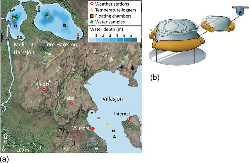
significantly between lakes (ANOVA, pJ. Jansen et al.: Drivers of diffusive CH4 emissions 1921 Figure 5. Time series of air and surface mixed-layer temperature (three-lake mean) (a), wind speed, gas transfer velocity from the surface renewal model (kmod and its buoyancy component, kmod,β ) and from chamber observations (kch ) (three-lake mean values, error bars repre- sent 95 % confidence intervals) (b), chamber CH4 flux (c), air–water CH4 concentration difference (d), precipitation and changes in water level in Mellersta Harrsjön (e), and the water temperature in Villasjön (f), Inre Harrsjön (g), and Mellersta Harrsjön (h) during the ice-free season of 2017 (1 June to 20 October). The white lines in panels (f–h) represent the depth of the surface mixed layer. Thin and thick lines in panels (a) and (b) represent half-hourly and daily means, respectively. In panel (a) only the half-hourly time series of Twater was plotted. iment temperature varied primarily on a seasonal timescale fer velocity reached its maximum value (Fig. 7b, d). How- (CV = 52 % and 45 %, n = 17) and less on diel timescales ever, binned means of the 1 h chamber fluxes (Fch (1 h)) were (CV = 3 % and 2 %, n = 24). Similar to the wind speed not significantly different at the 95 % confidence level (error the gas transfer velocity varied primarily on diel timescales bars) and did not show a clear diel pattern (Fig. 7b). Tem- (Fig. 7), albeit with a lower amplitude. This was in part poral patterns of fluxes and concentrations were very similar because kmod ∝ u3/4 (Eq. 4) and because the drag coeffi- between the lakes (Figs. S2 and S3). cient, used to compute the water-side friction velocity in Eq. 5, increases at lower wind speeds and under an unsta- 3.5 Timescale analysis ble atmosphere, which was typically the case. The surface concentration was correlated with wind speed and temper- The spectral density plot (Fig. 8a) disentangles dominant ature (Fig. 4f, g) and showed both seasonal and diel vari- timescales of variability of the drivers of the flux. The power ability. On diel timescales 1[CH4 ] and kmod were out of spectra of wind speed and temperature peaked at periods of phase; 1[CH4 ] peaked just before noon, when the gas trans- 1 d and 1 year, following well-known diel and annual cycles www.biogeosciences.net/17/1911/2020/ Biogeosciences, 17, 1911–1932, 2020
1922                                                                              J. Jansen et al.: Drivers of diffusive CH4 emissions

Figure 6. Scatter plots of the CH4 residence time (a–c) and storage (d–f) versus time, surface water temperature, and wind speed. Symbol
colours represent the different lakes. Large symbols represent binned means, and small symbols represent individual estimates. Bin sizes were
10 d, 1 ◦ C, and 0.5 m s−1 for time, water temperature, and U10 , respectively. Each storage observation was paired with T and U10 averaged
over the 24 h (Villasjön) and 72 h (Inre and Mellersta Harrsjön) prior to water sampling, reflecting average conditions during CH4 residence
times. The linear regressions of the residence time onto time (a) and temperature (b) were not statistically significant (p = 0.07–0.10). Linear
relations of binned quantities and U10 were statistically significant (c: p ≤ 0.002; f: p ≤ 0.04). Arrhenius-type functions (Eq. 7) adequately
described the storage-temperature relation in each lake (e: R 2 ≥ 0.70, p
J. Jansen et al.: Drivers of diffusive CH4 emissions                                                                         1923

of both the variability at < 1-week timescales (Fig. 7b) and      4.2   Drivers of flux
the value of σinit . Finally, the climacogram shows that kmod
retains about 72 % of its variability at 24 h timescales, which   Methane emitted from lakes in wetland environments can be
justifies our averaging over chamber deployment periods for       produced in situ or be transported in from the surrounding
comparison with kch and the computation of the model scal-        landscape (Paytan et al., 2015). The distinction is impor-
ing parameter α 0 (Fig. 3).                                       tant because some controls on terrestrial methane production,
                                                                  such as water table depth (Brown et al., 2014), are irrelevant
                                                                  in lakes. In the Stordalen Mire lakes, the Arrhenius-type re-
4     Discussion                                                  lation of CH4 fluxes and concentrations (Fig. 4b, f) together
                                                                  with short CH4 residence times (Fig. 6) suggest that efficient
4.1    Magnitudes of fluxes and gas transfer velocities
                                                                  redistribution of dissolved CH4 strongly coupled emissions
Overall, diffusive CH4 emissions from the Stordalen Mire          to sediment methane production. High CH4 concentrations
lakes (6.9 ± 0.3 mg m−2 d−1 , mean ±95 % CI) were lower           in the stream (Sect. 3.4) further suggest that external inputs
than the average of postglacial lakes north of 50◦ N,             of CH4 – produced in the fens and transported into the stream
but within the interquartile range (mean 12.5, IQR 3.0–           with surface runoff, or produced in stream sediments – may
17.9 mg m−2 d−1 ; Wik et al., 2016b). Emissions are also at       have elevated emissions in Mellersta Harrsjön (Lundin et
the lower end of the range for northern lakes of similar size     al., 2013). However, although the Mire exports substantial
(0.01–0.2 km2 ) (1–100 mg m−2 d−1 ; Wik et al., 2016b). As        quantities of dissolved organic carbon (DOC) and presum-
emissions of the Stordalen Mire lakes do not appear to be         ably CH4 from the waterlogged fens to the lakes (Olefeldt
limited by substrate quality or quantity (Wik et al., 2018),      and Roulet, 2012), after rainy periods we observed either
but strongly depend on temperature (Fig. 4b), the difference      no significant change in 1[CH4 ] (3–6 July and 21–27 Au-
is likely because a majority of flux measurements from other      gust 2017, Fig. 5) or a decrease (13–19 July 2017, Fig. 5). It
postglacial lakes were conducted in the warmer, subarctic bo-     remains unclear whether such reduced storage resulted from
real zone. Boreal lake CH4 emissions are generally higher         lower methanogenesis rates associated with the temperature
for lakes of similar size: 20–40 mg m−2 d−1 (binned means),       drop after rainfall, convection-induced degassing, or lake wa-
n = 91 (Rasilo et al., 2015) and ∼ 12 mg m−2 d−1 , n = 72         ter displacement or dilution by surface runoff.
(Juutinen et al., 2009).                                             Turbulent transfer was dominated by wind shear, and we
   The gas transfer velocity in the Stordalen Mire lakes was      computed a minor contribution (∼ 8 %) of the buoyancy-
similar to that predicted from wind-based models of Cole and      controlled fraction of k. Our result differs from that in Read
Caraco (1998) and Crusius and Wanninkhof (2003) at low            et al. (2012), who found that buoyancy flux dominated tur-
wind speeds (Fig. 9). Both were based on tracer experiments       bulence production in temperate lakes 0.1 km2 in size and
with sampling over several days and thus, like our approach,      smaller. For the Stordalen Mire lakes we computed higher
are integrative measures. The slope of the linear wind–kch        ice-free season mean values of u∗w , as well as lower values
relation (OLS: 0.81 ± 0.21, slope ±95 % CI, R 2 = 0.20 and        of the water-side vertical friction velocity, w∗w = (βzmix )1/3 ,
p
1924 J. Jansen et al.: Drivers of diffusive CH4 emissions
Figure 8. Timescale analysis of the diffusive CH4 flux and its drivers. (a) Normalized spectral density of whole-year near-continuous time
series of the air temperature (Tair ), temperature of the surface water and ice (0.1–0.5 m, Twater ), temperature of the surface sediment in
Mellersta Harrsjön (Tsed ), and wind speed (U10 ). (b) Climacogram of the measured and modelled CH4 flux (Fch , Fmod ), air and surface
water temperature (Tair , Twater ), water–air concentration difference (1[CH4 ]), modelled gas transfer velocity (kmod ), and wind speed (U10 )
during the ice-free seasons of 2009–2017. Dashed, light-grey curves represent (combinations of) trigonometric functions of mean 0 and
amplitude 1 with a specified period. The 24 h and 1-year harmonic functions were continuous over the dataset period while the 24 h + 1-
year harmonic was limited to periods when chamber flux data were available. Panel (a) is based on continuous time series that include the
ice-cover seasons: Fig. S4 shows spectral density plots for individual ice-free seasons.
implications for the choice of models or proxies of the flux in lasted from 23 June to 30 July 2014. Emissions during this
predictive analyses. For lakes that mix frequently and have a period comprised 29 %–56 % (depending on the lake) of
climatology similar to that of the Stordalen Mire (Malmer the 2014 ice-free diffusive flux, while the peak quantity of
et al., 2005), temperature-based proxies (e.g. Thornton et accumulated CH4 comprised < 5 %. Two mechanisms may
al., 2015) would resolve most of the variability of the ice- explain the lack of CH4 accumulation. First, stratification
free diffusive CH4 flux at timescales longer than a month. was frequently disrupted by vertical mixing (Fig. 5g–h), and
Advanced gas transfer models that account for atmospheric concurrent hypolimnetic CH4 concentrations were not sig-
stability and rapid variations in wind shear, such as we nificantly different from (Inre Harrsjön, 2010–2017, paired
have used here, allowed us to resolve variability in flux at t test, p = 0.12, n = 32) or lower than (Mellersta Harrsjön,
timescales shorter than about a month. Our results are repre- 2010–2017, paired t test, p25 and by
fluxes during heating and cooling are higher. 2 orders of magnitude for N >40 (MacIntyre et al., 2018),
kmod was only slightly lower (2.8 cm h−1 ) than the multi-
4.3 Storage and stability year mean (3.0 cm h−1 ). Thus, in weakly stratified lakes with
strong wind mixing, the temperature sensitivity of diffusive
The robust temperature sensitivity of lake methane emissions CH4 emissions may be observed without significant modula-
(Fig. 4b,f) (Wik et al., 2014; Yvon-Durocher et al., 2014) is tion by stratification.
driven by biotic and abiotic mechanisms. Lake mixing can Degassing (Fig. 4c, g) prevented an unlimited increase in
modulate temperature relations by periodically decoupling the emission rate with the gas transfer velocity. In this way,
production from emission rates (Engle and Melack, 2000). 1[CH4 ] acted as a negative feedback that maintained a quasi-
Here, enhanced CH4 accumulation during periods of strati- steady state between CH4 production and removal processes
fication may have contributed to concentration and storage throughout the ice-free season. In all three lakes CH4 resi-
maxima in July and August (Figs. 4e, 6d). However, as the dence times were inversely proportional to the wind speed
CH4 residence time was invariant over the season and with (Fig. 6c), indicating an imbalance between production and
temperature (Fig. 6a, b), the storage–temperature relation removal processes. We hypothesize that the imbalance ex-
(Fig. 6e) likely reflects rate changes in sediment methano- ists because the variability of wind speed peaked on shorter
genesis rather than inhibited mixing. For example, the high- timescales than that of the water temperature (Fig. 8a).
est CH4 concentrations in our dataset (59.1 ± 26.4 mg m−3 , Changes in wind shear periodically pushed the system out
n = 37) were measured during a period with exceptionally of production–emission equilibrium, allowing for transient
high surface water temperatures (Twater = 18.5 ± 3.6 ◦ C) that degassing and accumulation of dissolved CH4 . The temporal
Biogeosciences, 17, 1911–1932, 2020 www.biogeosciences.net/17/1911/2020/J. Jansen et al.: Drivers of diffusive CH4 emissions 1925
4.4 Timescales of variability
Overall, the short-term variability of the flux due to wind
speed (1.1–13.2 mg m−2 d−1 ) was similar to the long-
term variability due to temperature (0.7–12.2 mg m−2 d−1 )
(ranges of the binned means, Fig. 4b–c). The diel patterns
in the mixed-layer depth (Fig. 5) and the gas transfer veloc-
ity (Fig. 7d) and daytime variation in the surface concentra-
tion (Fig. 7b) were indicative of daily storage-and-release cy-
cles, resulting in a flux difference of about 5 mg m−2 d−1 be-
tween morning and afternoon, about half the mean seasonal
range (Fig. 7a). Diel variability of lake methane fluxes has
been observed at Villasjön (eddy covariance, Jammet et al.,
2017) and elsewhere (Bastviken et al., 2004, 2010; Crill et
al., 1988; Erkkilä et al., 2018; Eugster et al., 2011; Hamil-
Figure 9. Normalized gas transfer velocities (k600 ) versus the ton et al., 1994; Podgrajsek et al., 2014). Similarly, diel pat-
wind speed at 10 m (U10 ). Binned values (large rhombuses, kch terns in the gas transfer velocity have been inferred from
and kmod , bin size = 0.5 m s−1 ) and individual observations (small eddy covariance observations (Podgrajsek et al., 2015) and
rhombuses, kch ) from floating chambers (kch ) and the surface re- in model studies (Erkkilä et al., 2018). Apparent offsets be-
newal model (kmod with α 0 = 0.23). Error bars represent 95 % con- tween the diurnal peaks of the flux, surface concentrations,
fidence intervals of the binned means. Solid lines represent mod- and drivers (Fig. 7b, d) have been noted previously (Koeb-
els from the literature: Cole and Caraco (1998) (CC98), Crusius sch et al., 2015), but have yet to be explained. Continuous
and Wanninkhof (2003) (bilinear and power-law models) (CW03), eddy covariance measurements in lakes where the dominant
Soumis et al. (2008) (S08) and Vachon and Prairie (2013) (VP13)
emission pathway is turbulence-driven diffusion could help
for lake surface areas of 0.01 and 0.15 km2 . Supplement Table S1
lists the model equations and calibration ranges. A power-law re-
characterize flux variability on short timescales (e.g. Bar-
gression model is shown for the individual kch datapoints (n = 334): tosiewicz et al., 2015).
k600 = 0.77 × U101.02 + 0.62 (dashed yellow line). The CH4 residence times (1–3 d) were not much longer
than the diel timescale of vertical mixing (Fig. 5g, h). As
a result, horizontal concentration gradients developed in the
variability of dissolved gas concentrations is likely higher in deeper lakes (Table 2). The 23 ± 11 % concentration differ-
shallow wind-exposed systems with limited buffer capacity ence between depth zones in the deeper lakes (mean ±95 %
(Natchimuthu et al., 2016, 2017) and should be taken into Cl) fits transport model predictions of DelSontro et al. (2017)
account when applying gas transfer models to small lakes for small lakes (< 1 km2 ) that highlight the role of outgassing
and ponds. and oxidation during transport from production zones in the
Rapid degassing occurred at U10 ≥ 6.5 m s−1 (Fig. 4c). shallow littoral zones or the deeper sediments (Hofmann,
Gas fluxes at high wind speeds may have been enhanced by 2013). Concentration gradients may also have been caused
the kinetic action of breaking waves (Terray et al., 1996) or by physical processes, such as upwelling due to thermocline
through microbubble-mediated transfer. Wave breaking was tilting (Heiskanen et al., 2014). Higher-resolution measure-
observed on the Stordalen lakes at wind speeds ≥ 7 m s−1 . ments, for example with automated equilibration systems
Microbubbles of atmospheric gas (diameter < 1 mm) can (Erkkilä et al., 2018; Natchimuthu et al., 2016), are needed
form due to photosynthesis, rain, or wave breaking (Woolf to assess how much of the spatial and diel patterns of the
and Thorpe, 1991) and remain entrained for several days CH4 concentration can be explained by physical drivers such
(Turner, 1961). Due to their relatively large surface area, they as gas transfer and mixed-layer deepening (Eugster et al.,
quickly equilibrate with sparingly soluble gases in the water 2003; Vachon et al., 2019), or by biological processes such as
column, providing an efficient emission pathway to the at- methanogenesis and microbial oxidation (Ford et al., 2002).
mosphere when the bubbles rise to the surface (Merlivat and Gas transfer models can only deliver accurate fluxes if they
Memery, 1983). In inland waters microbubble emissions of are combined with measurements that capture the full spatio-
CH4 have only been indirectly inferred from differences in temporal variability of the surface concentration (Erkkilä et
CO2 and CH4 gas transfer velocities (McGinnis et al., 2015; al., 2018; Hofmann, 2013; Natchimuthu et al., 2016; Schilder
Prairie and del Giorgio, 2013), and more work is needed to et al., 2016). The short CH4 residence times and diel pattern
evaluate their significance in relatively sheltered systems. of 1[CH4 ] suggest that weekly sampling did not capture the
full temporal variability of the surface concentrations. Espe-
cially after episodes of high wind speeds and lake degassing
(Fig. 4c, g), concentrations may not have been representative
of the 24 h chamber deployment period.
www.biogeosciences.net/17/1911/2020/ Biogeosciences, 17, 1911–1932, 2020You can also read