Exploring how groundwater buffers the influence of heatwaves on vegetation function during multi-year droughts
←
→
Page content transcription
If your browser does not render page correctly, please read the page content below
Earth Syst. Dynam., 12, 919–938, 2021
https://doi.org/10.5194/esd-12-919-2021
© Author(s) 2021. This work is distributed under
the Creative Commons Attribution 4.0 License.

             Exploring how groundwater buffers the influence of
                 heatwaves on vegetation function during
                            multi-year droughts
              Mengyuan Mu1 , Martin G. De Kauwe1,2 , Anna M. Ukkola1 , Andy J. Pitman1 , Weidong Guo3 ,
                                       Sanaa Hobeichi1 , and Peter R. Briggs4
                   1 ARC Centre of Excellence for Climate Extremes and Climate Change Research Centre,
                                   University of New South Wales, Sydney 2052, Australia
                  2 School of Biological Sciences, University of Bristol, Bristol, BS8 1TQ, United Kingdom
           3 School of Atmospheric Sciences and Joint International Research Laboratory of Atmospheric and Earth

                                System Sciences, Nanjing University, Nanjing 210023, China
                  4 Climate Science Centre, CSIRO Oceans and Atmosphere, Canberra 2601, ACT, Australia

                               Correspondence: Mengyuan Mu (mu.mengyuan815@gmail.com)

                                        Received: 5 May 2021 – Discussion started: 6 May 2021
                           Revised: 29 July 2021 – Accepted: 3 August 2021 – Published: 13 September 2021

       Abstract. The co-occurrence of droughts and heatwaves can have significant impacts on many socioeconomic
       and environmental systems. Groundwater has the potential to moderate the impact of droughts and heatwaves by
       moistening the soil and enabling vegetation to maintain higher evaporation, thereby cooling the canopy. We use
       the Community Atmosphere Biosphere Land Exchange (CABLE) land surface model, coupled to a groundwater
       scheme, to examine how groundwater influences ecosystems under conditions of co-occurring droughts and heat-
       waves. We focus specifically on south-east Australia for the period 2000–2019, when two significant droughts
       and multiple extreme heatwave events occurred. We found groundwater plays an important role in helping veg-
       etation maintain transpiration, particularly in the first 1–2 years of a multi-year drought. Groundwater impedes
       gravity-driven drainage and moistens the root zone via capillary rise. These mechanisms reduced forest canopy
       temperatures by up to 5 ◦ C during individual heatwaves, particularly where the water table depth is shallow. The
       role of groundwater diminishes as the drought lengthens beyond 2 years and soil water reserves are depleted.
       Further, the lack of deep roots or stomatal closure caused by high vapour pressure deficit or high temperatures
       can reduce the additional transpiration induced by groundwater. The capacity of groundwater to moderate both
       water and heat stress on ecosystems during simultaneous droughts and heatwaves is not represented in most
       global climate models, suggesting that model projections may overestimate the risk of these events in the future.

1   Introduction                                                     2005), potentially accelerating tree die-off (Allen et al., 2010,
                                                                     2015; Birami et al., 2018), and setting conditions conducive
Droughts and heatwaves are important socioeconomic and               to wildfires (Jyoteeshkumar reddy et al., 2021). One region
environmental phenomena, impacting regional food produc-             experiencing severe coincident heatwaves and drought is
tion (Kim et al., 2019; Lesk et al., 2016), water resources          Australia (Mitchell et al., 2014). Drought in Australia is asso-
(Leblanc et al., 2009; Orth and Destouni, 2018), and the             ciated with large-scale modes of variability, including the El
resilience of ecosystems (Ibáñez et al., 2019; Ruehr et al.,         Niño–Southern Oscillation and the Indian Ocean Dipole (van
2019; Sandi et al., 2020). When droughts and heatwaves co-           Dijk et al., 2013), and periods of below-average rainfall can
occur (a “compound event”) the consequences can be partic-           extend for multiple years (Verdon-Kidd and Kiem, 2009).
ularly severe, reducing the terrestrial carbon sink (Ciais et al.,   Heatwaves are commonly synoptically driven, associated

Published by Copernicus Publications on behalf of the European Geosciences Union.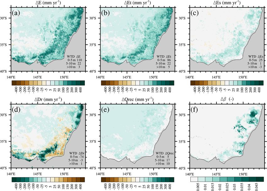
920                                             M. Mu et al.: Exploring how groundwater buffers the influence of heatwaves

with blocking events that can be sustained over many days         the influence of groundwater on droughts and heatwaves oc-
(Perkins-Kirkpatrick et al., 2016; Perkins, 2015). Modes of       curring at the same time (Keune et al., 2016; Zipper et al.,
variability and synoptic situations are important in setting      2019). Our key goal in this paper is therefore to examine the
up conditions conducive to drought and heatwave. However,         timescales and extent to which vegetation utilises ground-
once a heatwave or drought has become established, land–          water during drought and heatwaves and determine the de-
atmosphere interactions can intensify and prolong both heat-      gree to which groundwater can mitigate the impacts of com-
waves and droughts (Miralles et al., 2019), affect their inten-   pound extremes. We focus on droughts and heatwaves occur-
sity, and influence the risk of their co-occurrence (Mukher-      ring over south-eastern (SE) Australia during 2000–2019 us-
jee et al., 2020). The role of the land surface in amplifying     ing the Community Atmosphere Biosphere Land Exchange
or dampening heatwaves and droughts is associated with the        (CABLE) LSM. SE Australia is an ideal case study since
partitioning of available energy between sensible and latent      its forest and woodland ecosystems are known to be depen-
heat (Fischer et al., 2007; Hirsch et al., 2019) and is regu-     dent on groundwater (Eamus and Froend, 2006; Kuginis et
lated by subsurface water availability (Teuling et al., 2013;     al., 2016; Zencich et al., 2002), and it has experienced two
Zhou et al., 2019). As soil moisture becomes more limiting,       multi-year droughts and record-breaking heatwaves over the
more of the available energy is converted into sensible heat,     last 2 decades. By examining the role of groundwater in in-
reducing evaporative cooling via latent heat. Changes in the      fluencing droughts and heatwaves and by understanding how
surface turbulent energy fluxes influence the humidity in the     well CABLE can capture the relevant processes, we aim to
boundary layer, the formation of clouds, incoming solar ra-       build confidence in the simulations of land–atmosphere in-
diation, and the generation of rainfall (D’Odorico and Porpo-     teractions for future droughts and heatwaves.
rato, 2004; Seneviratne et al., 2010; Zhou et al., 2019). The
sensible heat fluxes warm the boundary layer, leading to heat
                                                                  2     Methods
that can accumulate over several days and exacerbate heat
extremes (Miralles et al., 2014), which can in turn increase      2.1    Study area
the atmospheric demand for water and intensify drought (Mi-
ralles et al., 2019; Schumacher et al., 2019).                    The climate over SE Australia varies from humid temper-
   Vegetation access to groundwater has the potential to al-      ate near the coast to semi-arid in the interior. In the last
ter these land–atmosphere feedbacks by maintaining vegeta-        20 years, SE Australia experienced the 9-year Millennium
tion function during extended dry periods, supporting tran-       Drought during 2001–2009 (van Dijk et al., 2013), where
spiration and moderating the impact of droughts and heat-         rainfall dropped from a climatological average (1970–1999)
waves (Marchionni et al., 2020; Miller et al., 2010). Where       of 542 to 449 mm yr−1 , and a 3-year intense recent drought
the water table is relatively shallow, capillarity may bring      during 2017–2019 where rainfall dropped to 354 mm yr−1
water from the groundwater towards the surface root zone,         (Fig. S1). It has also suffered record-breaking summer heat-
increasing plant water availability. Where the water table is     waves in 2009, 2013, 2017, and 2019 (Bureau of Meteo-
deeper, phreatophytic vegetation with tap roots can directly      rology, 2013, 2017, 2019; National Climate Centre, 2009).
access groundwater (Zencich et al., 2002). The presence of        Here we investigate groundwater interactions during the pe-
groundwater and the access to groundwater by vegetation are       riod 2000–2019, focusing on the Millennium Drought (MD,
therefore likely to buffer vegetation drought and heatwave        2001–2009) and the recent drought (RD, 2017–2019).
stress. For example, groundwater may help vegetation sus-
tain transpiration and consequently cool plant canopies via       2.2    Overview of CABLE
evaporation. This is particularly critical during compound
events where cessation of transpiration would increase the        CABLE is a process-based LSM that simulates the inter-
risk of impaired physiological function and the likelihood        actions between climate, plant physiology, and hydrology
that plants would exceed thermal limits and risk mortality        (Wang et al., 2011). Above ground, CABLE simulates the
(Geange et al., 2021; O’sullivan et al., 2017; Sandi et al.,      exchange of carbon, energy, and water fluxes, using a single-
2020).                                                            layer, two-leaf (sunlit and shaded) canopy model (Wang and
   Quantifying the influence of groundwater on vegetation         Leuning, 1998), with a treatment of within-canopy turbu-
function has remained challenging as concurrent observa-          lence (Raupach, 1994; Raupach et al., 1997). CABLE in-
tions of groundwater dynamics, soil moisture, and energy          cludes a six-layer soil model (down to 4.6 m) with soil hy-
and water fluxes are generally lacking over most of Australia     draulic and thermal characteristics dependent on the soil type
and indeed many parts of the world. Land surface models           and soil moisture content. CABLE has been extensively eval-
(LSMs) provide an alternative tool for studying the interac-      uated (e.g. Abramowitz et al., 2008; Wang et al., 2011; Zhang
tions between groundwater, vegetation, and surface fluxes in      et al., 2013) and benchmarked (Abramowitz, 2012; Best et
the context of heatwaves and droughts (Gilbert et al., 2017;      al., 2015) at global and regional scales.
Martinez et al., 2016a; Maxwell et al., 2011; Shrestha et al.,       Here we adopt a version of CABLE (Decker, 2015; Decker
2014). However, there has been very little work focused on        et al., 2017) which includes a dynamic groundwater compo-

Earth Syst. Dynam., 12, 919–938, 2021                                                 https://doi.org/10.5194/esd-12-919-2021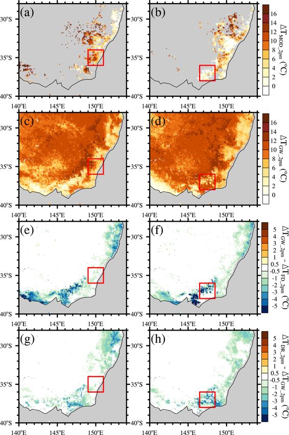
M. Mu et al.: Exploring how groundwater buffers the influence of heatwaves                                                    921

nent with aquifer water storage. This version, CABLE-GW,           where ddzl is the mean subgrid-scale slope, q̂sub is the maxi-
has been previously evaluated by Decker (2015), Ukkola et          mum rate of subsurface drainage (mm s−1 ), and fp is a tun-
al. (2016b), and Mu et al. (2021) and shown to perform well        able parameter. qsub is generated from the aquifer and the
for simulating water fluxes. CABLE code is freely available        saturated deep soil layers (below the third soil layer).
upon registration (https://trac.nci.org.au/trac/cable/wiki, last
access: 29 August 2021); here we use CABLE SVN revision
                                                                   2.4     Experiment design
7765.
                                                                   To explore how groundwater influences droughts and heat-
2.3   Hydrology in CABLE-GW                                        waves, we designed two experiments, with and without
                                                                   groundwater dynamics, driven by the same 3 h time-evolving
The hydrology scheme in CABLE-GW solves the vertical               meteorology forcing and the same land surface properties
redistribution of soil water via a modified Richards equation      (see Sect. 2.5 for datasets) for the period 1970–2019 at a
(Zeng and Decker, 2009):                                           0.05◦ spatial resolution with a 3 h time step. To correct a ten-
∂θ    ∂  ∂                                                         dency for high soil evaporation, we implemented a param-
   = − K (9 − 9E ) − Fsoil ,                                (1)    eterisation of soil evaporation resistance that has previously
∂t    ∂z ∂z
                                                                   been shown to improve the model (Decker et al., 2017; Mu
where θ is the volumetric water content of the soil                et al., 2021).
(mm3 mm−3 ), K is the hydraulic conductivity (mm s−1 ), z
is the soil depth (mm), 9 and 9E are the soil matric poten-        2.4.1    Groundwater experiment (GW)
tial (mm) and the equilibrium soil matric potential (mm), and
Fsoil is a sink term related to subsurface runoff and transpi-     This simulation uses the default CABLE-GW model, which
ration (s−1 ) (Zeng and Decker, 2009; Decker, 2015). To sim-       includes the unconfined aquifer to hold the groundwater stor-
ulate groundwater dynamics, an unconfined aquifer is added         age and simulates the water flux between the bottom soil
to the bottom of the soil column with a simple water balance       layer and the aquifer. We first ran the default CABLE-GW
model:                                                             with fixed CO2 concentrations at 1969 levels for 90 years by
                                                                   looping the time-evolving meteorology forcing over 1970–
dWaq                                                               1999. At the end of the 90-year spin-up, moisture in both the
     = qre − qaq,sub ,                                      (2)
 dt                                                                soil column and the groundwater aquifer reached an effec-
where Waq is the mass of water in the aquifer (mm), qaq,sub        tive equilibrium when averaged over the study area. We then
is the subsurface runoff in the aquifer (mm s−1 ), and qre is      ran the model from 1970 to 2019 with time varying CO2 . We
the water flux between the aquifer and the bottom soil layer       omit the first 30 years of this period and analyse the period
(mm s−1 ) computed by the modified Darcy’s law:                    2000–2019 to allow for further equilibrium with the time-
                                                                 evolving CO2 .
       (Kaq + Kbot ) 9aq − 9n − 9E,aq − 9E,n
qre =                                              ,      (3)
            2                 zwtd − zn                            2.4.2    Free drainage experiment (FD)

where Kaq and Kbot are the hydraulic conductivity in the           Many LSMs, including those used in the Coupled Model In-
aquifer and in the bottom soil layer (mm s−1 ), 9aq and 9E,aq      tercomparison Project 5 (CMIP5), still use a free drainage as-
are the soil matric potentials for the aquifer (mm), and 9n        sumption and neglect the parameterisation of the unconfined
and 9E,n are the soil matric potentials for the bottom soil        aquifer. To test the impact of this assumption we decoupled
layer (mm). zwtd and zn are the depth of the water table           the aquifer from the bottom soil layer and thus removed the
(mm) and the lowest soil layer (mm), respectively. The posi-       influence of groundwater dynamics (experiment FD). In FD,
tive qre refers to the downward water flow from soil column        at the interface between the bottom soil layer and the aquifer,
to aquifer (i.e. vertical drainage, Dr ), and the negative qre     soil water can only move downwards as vertical drainage at
is the upward water movement from the aquifer to the soil          the rate defined by the bottom soil layer’s hydraulic conduc-
column (i.e. recharge, Qrec ). CABLE-GW assumes that the           tivity:
groundwater aquifer sits above impermeable bedrock, giving
a bottom boundary condition of                                     qre = Kbot .                                                (6)

qout = 0.                                                   (4)    This vertical drainage is added to the subsurface runoff flux:

CABLE-GW computes the subsurface runoff (qsub , mm s−1 )           qsub = qsub + qre .                                         (7)
using
                                                                   The simulated water table depth (WTD, i.e. zwtd ) in CABLE-
             dz            z
                          − wtd
                             fp
                                                                   GW affects the water potential gradient between the soil lay-
qsub = sin      q̂sub e           ,                         (5)    ers via 9E (Zeng and Decker, 2009) and impacts qsub (Eq. 5).
             dl

https://doi.org/10.5194/esd-12-919-2021                                                  Earth Syst. Dynam., 12, 919–938, 2021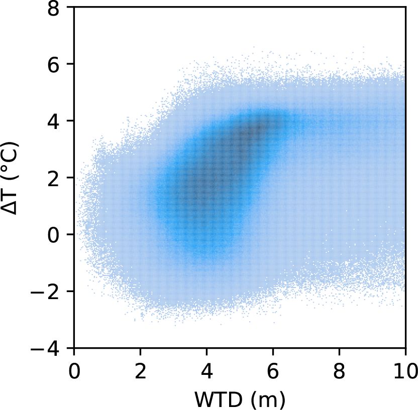
922                                               M. Mu et al.: Exploring how groundwater buffers the influence of heatwaves

However, in FD, decoupling the soil column from the aquifer         2.5   Datasets
and adding vertical drainage directly to subsurface runoff
causes an artificial and unrealistic decline in WTD. To solve       Our simulations are driven by the atmospheric forcing from
this problem, we assume a fixed WTD in the FD simulations           the Australian Water Availability Project (AWAP), which
at 10 m in order to remove this artefact from the simulation        provides daily gridded data covering Australia at 0.05◦ spa-
of 9E and qsub .                                                    tial resolution (Jones et al., 2009). This dataset has been
   The FD simulations are initialised from the near-                widely used to force LSMs for analysing the water and car-
equilibrated state at the end of the 90-year spin-up used in        bon balances in Australia (Haverd et al., 2013; De Kauwe et
GW. The period 1970–2019 is then simulated using varying            al., 2020; Raupach et al., 2013; Trudinger et al., 2016). The
CO2 and the last 20 years are used for analysis.                    AWAP forcing data include observed fields of precipitation,
                                                                    solar radiation, minimum and maximum daily temperatures,
2.4.3   Deep root experiment (DR)                                   and vapour pressure at 09:00 and 15:00. Since AWAP forcing
                                                                    does not include wind and air pressure we adopted the near-
The parameterisation of roots, including the prescription           surface wind speed data from McVicar et al. (2008) and as-
of root parameters in LSMs, is very uncertain (Arora and            sume a fixed air pressure of 1000 hPa. Due to missing obser-
Boer, 2003; Drewniak, 2019) and LSMs commonly employ                vations before 1990, the solar radiation input for 1970–1989
root distributions that are too shallow (Wang and Dickinson,        was built from the 1990–1999 daily climatology. Similarly,
2012). The vertical distribution of roots influences the de-        wind speeds for 1970–1974 are built from the 30-year clima-
gree to which plants can utilise groundwater, and potentially       tology from 1975 to 2004. We translated the daily data into
the role groundwater plays in influencing droughts and heat-        3-hourly resolution using a weather generator (Haverd et al.,
waves. To explore the uncertainty associated with root dis-         2013).
tribution, we added a “deep root” (DR) experiment by in-               The land surface properties for our simulations are
creasing the effective rooting depth in CABLE for tree areas.       prescribed based on observational datasets. Land cover type
In common with many LSMs, CABLE-GW defines the root                 is derived from the National Dynamic Land Cover Data of
distribution following Gale and Grigal (1987):                      Australia (DLCD) (https://www.ga.gov.au/scientific-topics/
             z                                                      earth-obs/accessing-satellite-imagery/landcover,          last
froot = 1 − βroot ,                                          (8)    access: 29 August 2021). We classify DLCD’s
                                                                    land cover types to five CABLE PFTs: crop (irri-
where froot is the cumulative root fraction (between 0 and
                                                                    gated/rainfed crop, pasture, and sugar DLCD classes),
1) from the soil surface to depth z (cm), and βroot is a fit-
                                                                    broadleaf evergreen forest (closed/open/scattered/sparse
ted parameter specified for each plant functional type (PFT)
                                                                    tree), shrub (closed/open/scattered/sparse shrubs and
(Jackson et al., 1996). In CABLE, the tree areas in our study
                                                                    open/scattered/sparse     chenopod      shrubs),    grassland
region are simulated as evergreen broadleaf PFT (Fig. S2a)
                                                                    (open/sparse herbaceous), and barren land (bare areas).
with a βroot = 0.962, implying that only 8 % of the simulated
                                                                    We then resample the DLCD dataset from the 250 m res-
roots are located below the soil depth of 0.64 m (Fig. S2b).
                                                                    olution to the 0.05◦ resolution. The leaf area index (LAI)
However, field observations (Canadell et al., 1996; Eberbach
                                                                    in CABLE is prescribed using a monthly climatology
and Burrows, 2006; Fan et al., 2017; Griffith et al., 2008)
                                                                    derived from the Copernicus Global Land Service product
suggest that the local trees tend to have a far deeper root sys-
                                                                    (https://land.copernicus.eu/global/products/lai, last access:
tem, possibly to help cope with the high climate variability.
                                                                    29 August 2021). The climatology was constructed by first
We therefore increased βroot for the evergreen broadleaf PFT
                                                                    creating a monthly time series by taking the maximum of
to 0.99, which assumes 56 % of roots are located at depths
                                                                    the 10 daily time steps each month and then calculating a
below 0.64 m and 21 % of roots below 1.7 m (Fig. S2b). This
                                                                    climatology from the monthly data over the period 1999–
enables the roots to extract larger quantities of deep soil water
                                                                    2017. The LAI data were resampled from the original 1 km
moisture, which is more strongly influenced by groundwater.
                                                                    resolution to the 0.05◦ resolution following De Kauwe et
   Given that we lack the detailed observations to set root dis-
                                                                    al. (2020). Soil parameters are derived from the soil texture
tributions across SE Australia, we undertake the DR exper-
                                                                    information (sand, clay, and silt fraction) from SoilGrids
iment as a simple sensitivity study. We only run this exper-
                                                                    (Hengl et al., 2017) via the pedotransfer functions in Cosby
iment during January 2019, when the record-breaking heat-
                                                                    et al. (1984) and resampled from 250 m to 0.05◦ resolution.
waves compound with the severe recent drought. The DR ex-
                                                                       To evaluate the model simulations, we use monthly to-
periment uses identical meteorology forcing and land surface
                                                                    tal water storage anomaly (TWSA) at 0.5◦ spatial resolu-
properties as GW and FD and is initialised by the state of the
                                                                    tion from the Gravity Recovery and Climate Experiment
land surface on the 31 December 2018 from the GW experi-
                                                                    (GRACE) and GRACE Follow On products (Landerer et al.,
ment.
                                                                    2020; Watkins et al., 2015; Wiese et al., 2016, 2018). The
                                                                    RLM06M release is used for February 2002–June 2017 and
                                                                    for June 2018–December 2019. We also use total land evap-

Earth Syst. Dynam., 12, 919–938, 2021                                                 https://doi.org/10.5194/esd-12-919-2021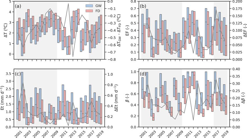
M. Mu et al.: Exploring how groundwater buffers the influence of heatwaves                                                 923

otranspiration from the 2000–2018 monthly Derived Opti-         pared to GRACE (47.74 mm) or GW (47.67 mm), particu-
mal Linear Combination Evapotranspiration (DOLCE ver-           larly during the wetter periods (2000, 2011–2016) and the
sion 2, Hobeichi et al., 2021a) at 0.25◦ resolution, as well    first ∼ 2 years of the droughts (2001–2002, 2017–2018)
as the 2000–2019 daily Global Land Evaporation Amster-          (Fig. 1a). This underestimation in FD compared to GW is
dam Model (GLEAM version 3.5, https://www.gleam.eu/;            linked to the lack of aquifer water storage in the FD sim-
Martens et al., 2017; Miralles et al., 2011) at 0.5◦ spa-       ulations, which provides a reservoir of water that changes
tial resolution. For daytime land surface temperature (LST)     slowly and has a memory of previous wet/dry climate condi-
we use the Moderate Resolution Imaging Spectroradiometer        tions (Fig. 1a).
(MODIS) datasets from Terra and Aqua satellites (products          Figure 1b shows the accumulated precipitation (P ) minus
MOD11A1 and MYD11A1, Wan and Li, 1997; Wan et al.,              evapotranspiration (E) over the two drought periods. GW in-
2015a, b) at 1 km spatial resolution. We only consider pix-     creases the evapotranspiration relative to FD such that the
els and time steps identified as good quality (QC flags 0).     accumulated P –E decreases from about 786 to 455 mm dur-
Only the daytime LST values are used due to the lack of         ing the Millennium Drought, which is within the range of
good-quality nighttime LST data. The Terra overpass occurs      DOLCE (460 mm) and GLEAM (97 mm) estimates. A sim-
at 10:00 and Aqua at 14:00 local time. To analyse the com-      ilar result, although over a much shorter period, is also ap-
pound events in January 2019, we linearly interpolate the 3-    parent for the recent drought (Fig. 1b). The lower P –E in
hourly model outputs to 14:00 to match the overpass time of     GW suggests that the presence of groundwater storage can
the Aqua LST. The GRACE, GLEAM, and MODIS datasets              alleviate the vegetation water stress during droughts and re-
were resampled to the AWAP resolution using bilinear inter-     duces the reliance of E on P , indicated by a small reduction
polation.                                                       in the correlation (r) between E and P from 0.28 in FD to
   To evaluate model performance during heatwaves, we           0.24 in GW for MD and a reduction from 0.42 to 0.37 for
identify heatwave events using the excess heat factor index     RD (Fig. 1b). Although the evapotranspiration products dis-
(EHF, Nairn and Fawcett, 2014). EHF is calculated using the     play some differences, the GW simulations are closer overall
daily AWAP maximum temperature, as the product of the dif-      to both the DOLCE and the GLEAM observationally con-
ference of the previous 3 d mean to the 90th percentile of      strained estimates. The better match of GW than FD to the
the 1970–1999 climatology and the difference of the previ-      two evapotranspiration products implies that adding ground-
ous 3 d mean to the preceding 30 d mean. A heatwave occurs      water improves the simulations during droughts, whilst the
when the EHF index is greater than 0 for at least 3 consec-     remaining mismatch would tend to suggest further biases in
utive days. We only focus on summer heatwaves occurring         simulated evapotranspiration arising from multiple sources
between December and February of the following year.            (e.g. a mismatch in leaf area index or contributions from the
                                                                understorey). The difference in E is also demonstrated spa-
                                                                tially in Fig. S3. During the Millennium Drought, the GW
3     Results
                                                                simulations show a clear improvement over FD in two as-
3.1    Simulations for the Millennium Drought and the
                                                                pects. GW shows smaller biases in E along the coast where
       recent drought
                                                                FD underestimates E strongly (Fig. S3b–c). The areas where
                                                                E is underestimated are also smaller in extent in GW, sug-
Previous studies have shown that simulations by LSMs di-        gesting that GW overall reduces the dry bias. The magni-
verge as the soil dries (Ukkola et al., 2016a), associated      tude of the bias in GW reaches around 300 mm over small
with systematic biases in evaporative fluxes and soil mois-     areas of SE Australia, while in the FD simulations biases are
ture states in the models (Mu et al., 2021; Swenson and         larger, reaching 400 mm over a larger area. Plant photosyn-
Lawrence, 2014; Trugman et al., 2018). We therefore first       thesis assimilation rates are associated with transpiration via
evaluate how well CABLE-GW captures the evolution of ter-       stomata conductance. Figure S4 presents the spatial maps of
restrial water variability during two recent major droughts.    gross primary productivity (GPP) during the two droughts.
   Figure 1a shows the total water storage anomaly during       GW simulations increase carbon uptake by 50–300 g C yr−1
2000–2019 observed by GRACE and simulated in GW and             along the coasts (Fig. S4c, f). However, since CABLE uses a
FD. Both GW and FD accurately capture the interannual           prescribed LAI and does not simulate any feedback between
variability in total water storage for SE Australia (r = 0.96   water availability and plant growth (e.g. defoliation) and its
in GW and 0.90 in FD). Both model configurations simulate       impact on GPP, we only focus on how GW influences evap-
a decline in TWSA through the first drought period (up to       otranspiration and the surface energy balance in the subse-
2009, see Fig. S1), the rapid increase in TWSA from 2010 as-    quent sections.
sociated with higher rainfall, a decline from around 2012 due      Overall, Figs. 1 and S3 indicates that representing ground-
to the re-emergence of drought conditions, and the rapid de-    water in the model improves the simulation of the interannual
cline during the recent drought after conditions had eased in   variability in the terrestrial water cycle and storage, particu-
2016 (Fig. S1). FD underestimates the magnitude of monthly      larly during droughts.
TWSA variance (standard deviation, SD = 37.18 mm) com-

https://doi.org/10.5194/esd-12-919-2021                                            Earth Syst. Dynam., 12, 919–938, 2021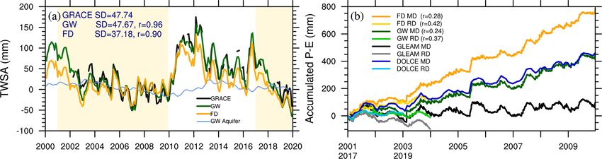
924                                                M. Mu et al.: Exploring how groundwater buffers the influence of heatwaves

Figure 1. (a) Total water storage anomaly (TWSA) during 2000–2019 and (b) accumulated P –E for the two droughts over SE Australia. In
panel (a), observations from GRACE are shown in black, the GW simulation in green, FD in orange, and the aquifer water storage anomaly
in GW in blue. The shading in panel (a) highlights the two drought periods. The left top corner of panel (a) displays the correlation (r)
between GRACE and GW/FD, as well as the standard deviation (SD, mm) of GRACE, GW, and FD over the periods when GRACE and the
simulations coincide. Panel (b) shows the accumulated P –E for two periods; the dark lines show the 2001–2009 Millennium Drought (MD)
and the light lines show the 2017–2019 recent drought (RD). The correlation (r) between the P and E is shown in the legend of panel (b).

3.2   The role of groundwater in sustaining                            areas where WTD is ∼ 5 m. This is associated with the WTD
      evapotranspiration during droughts                               being slightly below the bottom of the soil column (4.6 m).
                                                                       When the groundwater aquifer is nearly full in GW, the wet-
We next explore the mechanisms by which including ground-              ter soil in the bottom layer leads to a much higher hydraulic
water modifies the simulation of evapotranspiration. Figure 2          conductivity in GW than in FD, leading to higher vertical
displays the overall influence of groundwater on water fluxes          drainage in GW and a positive 1Dr . Inland, where the WTD
during the recent drought. GW simulates 50–200 mm yr−1                 tends to be much deeper there is no significant difference in
more E over coastal regions where there is high tree cover             Dr between GW and FD.
(Fig. 2a; see Fig. S2a for land cover). Adding groundwa-                  Figure 2e shows the difference in recharge into the
ter also increases E in most other regions, although the               upper soil column (1Qrec ) between GW and FD. The
impact is negligible in many inland and non-forested re-               recharge from the aquifer into the bottom soil layer provides
gions (i.e. west of 145◦ E). We identified a clear connec-             17 mm yr−1 of extra moisture in GW, where the WTD is be-
tion between E (Fig. 2a) and the simulated WTD in the                  tween 5–10 m, and 10 mm yr−1 where the WTD is < 10 m,
GW simulations (Fig. S5). GW simulates 110 mm yr−1 more                partially explaining the changes in E and Et in areas with
E when the WTD is shallower than 5 m deep, 22 mm yr−1                  a deep WTD. However, there is no significant 1Qrec in re-
when the WTD is 5–10 m deep, but only 3 mm yr−1 more                   gions with a shallow WTD (∼ 5 mm yr−1 ), suggesting the
when the WTD is below 10 m. Higher transpiration (Et )                 influence of groundwater is mainly via reduced drainage in
in GW explains 78 % of the evapotranspiration difference               these locations. Recharge from the aquifer to the soil column
between GW and FD where WTD is shallower than 5 m                      can only occur when WTD is below the soil column (bot-
(Fig. 2b). This is confirmed by the change in the soil evapo-          tom boundary at 4.6 m depth). If WTD is shallow and within
ration (1Es ) (Fig. 2c) where adding groundwater increases             the soil column, the interface is saturated and no recharge
Es by negligible amounts over most of SE Australia but by              from the aquifer to the soil column can occur and water only
up to 25 mm yr−1 in regions underlain by shallow ground-               moves downwards by gravity.
water (Fig. S5), which is consistent with field observations              The combined impact of reduced drainage in GW (Fig. 2d)
that indicate that Es can be substantial under conditions of a         and recharge from the aquifer into the root zone (Fig. 2e)
very shallow water table (Thorburn et al., 1992). In the very          is an increased water potential gradient between the drier
shallow WTD areas, the excess Es in GW results from the                top soil layers and the wetter deep soil layers, encouraging
capillary rise of moisture from the shallow groundwater to             overnight capillary rise. Taking the hot and dry January 2019
the surface.                                                           as an example, when the compound events occurred, Fig. 2f
   A significant factor in explaining how groundwater influ-           shows the maximum water stress factor difference (1β)
ences E is through changes in vertical drainage and recharge           overnight (between 21:00 and 03:00, i.e. predawn when soil
from the aquifer to the soil column. Figure 2d shows that the          is relatively moist following capillary lift overnight). We only
vertical drainage (Dr ) both increases and decreases depend-           consider rainless nights to exclude the impact of drainage in-
ing on the location. The addition of groundwater reduces ver-          duced by precipitation. The water stress factor (β) is based
tical drainage by 74 mm yr−1 where WTD is shallower than               on the root distribution and moisture availability in each soil
5 m. In some regions, the drainage increases with the inclu-           layer and represents the soil water stress on transpiration as
sion of groundwater by up to 100 mm yr−1 , especially in the           water becomes limiting. Figure 2f implies that while the re-

Earth Syst. Dynam., 12, 919–938, 2021                                                     https://doi.org/10.5194/esd-12-919-2021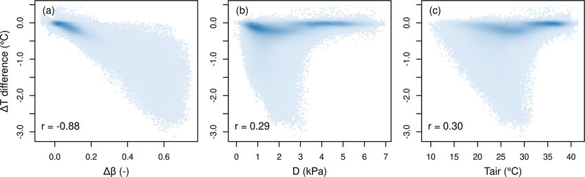
M. Mu et al.: Exploring how groundwater buffers the influence of heatwaves 925
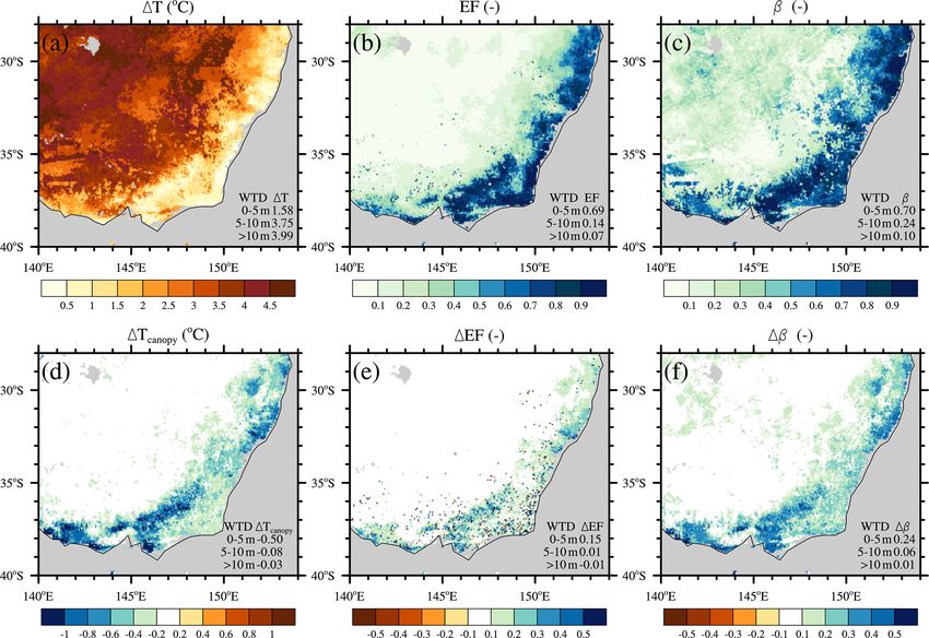
Figure 2. The overall influence of groundwater during the recent drought. Panels (a)–(e) are the difference (GW–FD) in evapotranspiration
(1E), transpiration (1Et ), soil evaporation (1Es ), vertical drainage (1Dr ) and recharge from the aquifer to soil column (1Qrec ), respec-
tively. In the bottom right of panels (a)–(e), the average of each variable over selected water table depths (WTDs) is provided. Panel (f) is the
maximum nighttime water stress factor difference (1β) between 03:00 (i.e. predawn when the soil is relatively moist following capillary lift
overnight) and 21:00 the previous day. We only include rainless nights in January 2019 to calculate 1β to remove any influence of overnight
rainfall.
distribution of moisture is small overall, in some locations it fect, from an average reduction of 0.52 ◦ C of the first 3 years
can reduce moisture stress by up to 4 %–6 %. to 0.16 ◦ C of the last 3 years in the Millennium Drought
(Fig. 3a). The impact of groundwater is clear in the evapora-
tive fraction (Fig. 3b) where in periods of higher rainfall (e.g.
3.3 The impact of groundwater during heatwaves 2010–2011; Fig. S1) and at the beginning of a drought (2001,
We next explore whether the higher available moisture due to 2017) the evaporative fraction (EF) is higher (0.03 to 0.18).
the inclusion of groundwater enables the canopy to cool itself This implies that more of the available energy is exchanged
via evapotranspiration during heatwaves by examining the with the atmosphere in the form of latent rather than sensible
temperature difference between the simulated canopy tem- heat. However, the strength of the cooling effect decreases
perature (Tcanopy , ◦ C) and the forced air temperature (Tair , as the droughts extend and the transpiration difference (1Et ,
◦ C). We focus on the forested regions (Fig. S2a) as the role of mm d−1 ) diminishes quickly (Fig. 3c) because the vegetation
groundwater in enhancing plant water availability was shown becomes increasingly water-stressed (Fig. 3d) which conse-
to be largest in these regions (Fig. 2). quently limits transpiration. For all variables (1T , EF, Et ,
Figure 3a shows the average Tcanopy − Tair (1T , ◦ C) over and β), the difference between GW and FD is greatest during
the forested regions for summer heatwaves from the GW and the wetter periods (e.g. 2013) and in the first 1–2 years of the
FD simulations, with the grey line indicating the median 1T multi-year drought (2001–2002 for the Millennium Drought
difference. During heatwaves, the inclusion of groundwater or 2017–2018 for the recent drought). After the drought be-
moistens the soil and supports higher transpiration, cooling comes well established, the FD and GW simulations con-
the canopy and reducing 1T relative to FD by up to 0.76 ◦ C verge as depleting soil moisture reservoirs reduce the impact
(e.g. summer heatwaves in 2013). As the drought lengthens of groundwater on canopy cooling and evaporative fluxes.
in time, the depletion of moisture gradually reduces this ef-
https://doi.org/10.5194/esd-12-919-2021 Earth Syst. Dynam., 12, 919–938, 2021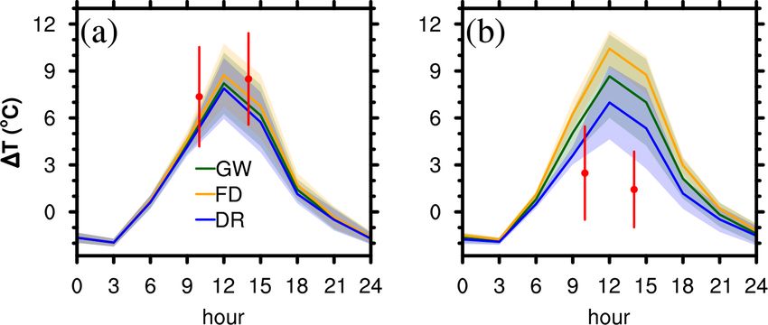
926                                                   M. Mu et al.: Exploring how groundwater buffers the influence of heatwaves

Figure 3. Groundwater-induced differences in (a) Tcanopy − Tair (1T ), (b) evaporative fraction (EF), (c) transpiration (Et ), and (d) water
stress factor (β) during 2000–2019 summer heatwaves over forested areas (the green region in Fig. S2a). The left y axis is the scale for boxes.
The blue boxes refer to the GW experiment and the red boxes to FD. For each box, the middle line is the median, the upper border is the 75th
percentile, and the lower border is 25th percentile. The right y axis is the scale for the grey lines which display the difference in the medians
(GW–FD). The shadings highlight the two drought periods.

   Figure 4a shows the spatial map of 1T simulated in GW                   less implies a threshold of ∼ 6 m, whereafter there is a de-
during heatwaves in the 2017–2019 drought. It indicates that               coupling and little influence from groundwater during heat-
both land cover type (Fig. S2a) and WTD (Fig. S5) contribute               waves. However, the absolute value of the threshold is likely
to the 1T pattern. The evaporative cooling via transpiration               CABLE-specific and associated with the assumption of a
is stronger over the forested areas compared to cropland or                4.6 m soil depth, which also sets the maximum rooting depth
grassland and stronger in the regions with a wetter soil as-               (roots can only extend to the bottom of the soil and cannot di-
sociated with a shallower WTD. However, EF is mainly de-                   rectly access the groundwater aquifer in CABLE). The CA-
termined by WTD (compare Figs. 4b and S5). Inland, where                   BLE soil depth comes from observational evidence of most
the WTD is deeper and the soil is drier, most of the net radia-            roots being situated within the top 4.6 m (Canadell et al.
tion absorbed by the land surface is partitioned into sensible             1996). Since the model assumes no roots exist in the ground-
rather than latent heat (Fig. 4b). However, in the coastal re-             water aquifer, when the water table is below this depth, the
gions with a shallow WTD, the wetter soil reduces the water                water fluxes become largely uncoupled between the soil col-
stress (Fig. 4c), enables a higher EF (Fig. 4b), and alleviates            umn and the groundwater aquifer, leading to a negligible im-
heat stress on the leaves (Fig. 4a). Along the coast where                 pact of GW below ∼ 6 m depth.
WTD is shallow, GW simulates a cooler canopy temperature
due to the higher evaporative cooling (Fig. 4e), which is the
consequence of a lower soil water stress (Fig. 4f) linked to
the influence of groundwater (Fig. S5).                                    3.4   The impact of groundwater during the drought and
   Figure 5 shows the density scatter plot of 1T versus WTD                      heatwave compound events
in SE Australia forested areas during heatwaves in 2000–
2019. A shallow WTD moderates the temperature difference                   To examine the influence of groundwater on heatwaves oc-
between the canopy and the ambient air during heatwaves                    curring simultaneously with drought, we focus on a case
leading to a smaller temperature difference. Meanwhile, as                 study of the record-breaking heatwaves in January 2019,
the WTD increases, due to the limited rooting depth in the                 which is the hottest month on record for the study region (Bu-
model, the ability of the groundwater to support transpira-                reau of Meteorology, 2019). The unprecedented prolonged
tion and offset the impact of high air temperatures is reduced.            heatwave period started in early December 2018 and contin-
Figure 5 shows a large amount of variations but nonethe-                   ued through January 2019 with three peaks. We select 2 d
                                                                           (15 and 25 January 2019), when heatwaves spread across

Earth Syst. Dynam., 12, 919–938, 2021                                                           https://doi.org/10.5194/esd-12-919-2021
M. Mu et al.: Exploring how groundwater buffers the influence of heatwaves 927
Figure 4. Land response to heatwaves during the recent drought. Panels (a)–(c) are the mean Tcanopy − Tair (1T ), evaporative fraction (EF),
and soil water stress factor (β) in GW, respectively, during 2017–2019 summer heatwaves. Panels (d)–(f) are the difference (GW–FD) of
Tcanopy , EF, and β. In the bottom right of each plot, the average of each variable over selected water table depths (WTDs) is provided. Note
that the colour bar is switched between (d) and (e)–(f).
atures, but note that this comparison is not direct as the
satellite estimate will contain contributions from the under-
storey and soil. Figure 6a–b show the good-quality MODIS
LST minus Tair at 14:00 (1TMOD_14:00 ) over forested regions
on the 15 and 25 January 2019, and Fig. 6c–d display the
matching GW-simulated 1T at 14:00 (1TGW_14:00 ). Overall,
1TGW_14:00 increases from the coast to the interior in both
heatwaves, consistent with the 1TMOD_14:00 pattern in both
heatwaves, although 1TGW_14:00 appears to be biased high
relative to 1TMOD_14:00 along the coastal forests (Fig. S7a–
b).
Figure 6e–f show the 1T14:00 difference between GW and
FD. Access to groundwater can reduce canopy temperature
Figure 5. A density scatter plot of Tcanopy −Tair (1T ) versus water
by up to 5 ◦ C, in particular where the WTD is shallow. While
table depth (WTD) in GW simulations over forested areas in all
reductions of 5 ◦ C are clearly limited in spatial extent, the
heatwaves during 2000–2019. Every tree pixel on each heatwave
day accounts for one record, and the darker colours show higher overall pattern of cooling is quite widespread and coincident
recorded densities. with the groundwater-induced Et increase (Fig. S8a–b), im-
plying a reduction in heat stress along coastal regions with
a shallow WTD during heatwaves. Generally, GW matches
the study region, from the second and third heatwave phases MODIS LST better than FD despite the bias in both simu-
(Fig. S6). lations (compare Figs. S7a–b and S7c–d). Nevertheless, the
We evaluate CABLE Tcanopy against MODIS LST ob- temperature reduction between GW and FD is still modest
servations, concentrating on forested areas where MODIS (< 1 ◦ C) for most of the forested regions. This may be re-
LST should more closely reflect vegetation canopy temper- lated to the shallow root distribution assumed in many LSMs,
https://doi.org/10.5194/esd-12-919-2021 Earth Syst. Dynam., 12, 919–938, 2021928 M. Mu et al.: Exploring how groundwater buffers the influence of heatwaves Figure 6. The simulation of two heatwaves on 15 (left column) and 25 January 2019 (right column). The first row shows the difference between MODIS land surface temperature (LST) and Tair at 14:00 (1TMOD_14:00 ) (only forested areas with good LST quality data are displayed). The second row is the GW simulation of 1T at 14:00 (1TGW_14:00 ). The third row is the difference of 1T at 14:00 between GW and FD simulations (1TGW_14:00 − 1TFD_14:00 ). The last row is the same as the third row but for the difference between the DR and GW simulations (1TDR_14:00 − 1TGW_14:00 ). Note that the comparison between GW/FD/DR and MODIS LST is shown in Fig. S7. Earth Syst. Dynam., 12, 919–938, 2021 https://doi.org/10.5194/esd-12-919-2021
M. Mu et al.: Exploring how groundwater buffers the influence of heatwaves                                                      929

                                                                      3.5    Constraints on groundwater mediation during the
                                                                             compound events

                                                                      We finally probe the reasons for the apparent contradic-
                                                                      tion between the large impact of groundwater on E during
                                                                      drought (Fig. 2a) but a smaller impact on 1T during the
                                                                      compound events (Fig. 7). Figure 8 shows three factors (β,
                                                                      vapour pressure deficit (D), and Tair ) that constrain the im-
                                                                      pact of groundwater on 1T in CABLE during heatwaves in
                                                                      January 2019. Figure 8a shows the difference in 1T between
Figure 7. Diurnal cycle of 1T on 15 (left column) and 25 January      GW and FD as a function of 1β, suggesting that the inclu-
2019 (right column) over the selected regions shown in Fig. 6. The    sion of groundwater has a large impact on 1T when there
shadings show the uncertainty in every simulation defined as one
                                                                      is a coincidental and large difference in β between the GW
standard deviation (SD) among the selected pixels. The red dots are
MODIS LST minus Tair with the uncertainty shown by the red error
                                                                      and FD simulations. Figure 8b indicates a clear threshold at
bars. For both regions, only pixels available in MODIS are shown.     D = 3 kPa where GW and FD converge, while Fig. 8c shows
                                                                      a convergence threshold when Tair exceeds 32 ◦ C. Above
                                                                      these two thresholds, access to groundwater seemingly be-
which prevents roots from directly accessing the moisture             comes less important in mitigating plant heat stress. There
stored in the deeper soil (note, CABLE assumes 92 % of a              are two mechanisms in CABLE that explain this behaviour.
forest’s roots are in the top 0.64 m, Fig. S2b). To examine           First, as D increases, CABLE predicts that stomata begin
this possibility, we performed the deep root (DR) sensitivity         to close following a square root dependence (De Kauwe et
experiment which prescribed more roots in the deeper soil             al., 2015; Medlyn et al., 2011). Second, as Tair increases,
for forests (56 % below 0.64 m depth). Figure 6g–h illustrate         photosynthesis becomes inhibited as the temperature exceeds
the difference between 1T14:00 in DR and 1TGW_14:00 . By              the optimum for photosynthesis. In both instances, evapora-
enabling access to moisture in the deeper soil, the LSM sim-          tive cooling is reduced, regardless of the root zone moisture
ulates further cooling by 0.5–5 ◦ C across the forests associ-        state dictated by groundwater access. That is to say, access
ated with an Et increase of 25–250 W m−2 (Fig. S8c–d). The            to groundwater has limited capacity to directly mediate the
prescribed deeper roots also lead to an overall better simula-        heat stress on plants during a compound event when the air
tion of 1T at 20:00 relative to the MODIS LST (Figs. S7e–f            is very dry or very hot.
vs. Fig. S7a–b).
   Figure 7 shows the diurnal cycles of 1T for the two                4     Discussion
selected regions (red boxes in Fig. 6) compared with the
MODIS LST estimates. The region highlighted for the                   In the absence of direct measurements, we used the CABLE-
15 January (Fig. 7a) has a WTD of 4–7 m, while the region             GW LSM, constrained by satellite observations to investi-
highlighted for the 25 January (Fig. 7b) has a WTD < 4 m              gate how groundwater influences ecosystems under condi-
(Fig. S5). In both regions, the simulated 1T is highest in            tions of co-occurring droughts and heatwaves. We found
FD, lower in GW and lowest in DR. Where the WTD is                    that the influence of groundwater was most important dur-
4–7 m (Fig. 7a), the three simulated 1T are slightly lower            ing the wetter periods and the first ∼ 2 years of a multi-year
than 1T calculated by MODIS LST (red squares). How-                   drought (∼ 2001–2002 and 2017–2018; Figs. 1 and 3). This
ever, in the shallower WTD region (Fig. 7b), the simulated            primarily occurred via impedance of gravity-driven drainage
1T between experiments is more dispersed across experi-               (Fig. 2d) but also via capillary rise from the groundwater
ments and exceeds the MODIS 1T at both time points, im-               aquifer (Fig. 2e). This moistening enabled the vegetation to
plying that neglecting groundwater dynamics and deep roots            sustain higher E for at least a year (Fig. S9). As the droughts
is more likely to cause an overestimation of heat stress in the       progressed into multi-year events, the impact of groundwater
shallower WTD region. The shallower WTD region (Fig. 7b)              diminished due to a depletion of soil moisture stores regard-
tends to have a high LAI coverage, implying that the MODIS            less of whether groundwater dynamics were simulated.
LST represents a good approximation of the canopy temper-                When a heatwave occurs during a drought, and in partic-
ature over this region. Consequently, the lower MODIS 1T              ular early in a drought, the extra transpiration enabled by
implies that CABLE is likely underestimating transpiration,           representing groundwater dynamics helps reduce the heat
leading to an overestimation of 1T in all three simulations.          stress on vegetation (e.g. the reduction of 0.64 ◦ C of 1T
                                                                      over the forests in 2002, Fig. 3a). This effect is particularly
                                                                      pronounced in regions with a shallower WTD (e.g. where
                                                                      the groundwater was within the first 5 m, there was a 0.5 ◦ C
                                                                      mean reduction in 1T in the recent drought; Fig. 4d). Im-
                                                                      portantly, the role played by groundwater diminishes as the

https://doi.org/10.5194/esd-12-919-2021                                                  Earth Syst. Dynam., 12, 919–938, 2021
930 M. Mu et al.: Exploring how groundwater buffers the influence of heatwaves
Figure 8. Density scatter plots showing the three factors that influence the difference in Tcanopy − Tair between GW and FD (1T , expressed
as GW–FD difference). Panel (a) is 1T difference against the β difference (GW–FD) (1β), (b) is 1T difference against vapour pressure
deficit (D), and (c) is 1T difference against Tair . Each point corresponds to a tree pixel on a heatwave day in January 2019. The darker
colours illustrate where the records are denser. The correlation (r) between the x and y axes is shown in the bottom left of each panel.
drought lengthens beyond 2 years (Fig. 3). Additionally, ei- 2019; Seneviratne et al., 2010). Our results add to the knowl-
ther the lack of deep roots or stomatal closure caused by edge by quantifying the extent of the groundwater control,
high D/Tair can reduce the additional transpiration induced and eliciting the timescales of influence and the mechanisms
by groundwater. The latter plant physiology feedback dom- at play. The importance of vegetation–groundwater interac-
inates during heatwaves co-occurring with drought, even if tions on multi-year timescales has been identified previously.
the groundwater’s influence has increased root zone water Humphrey et al. (2018) hypothesised that climate models
availability. may underestimate the amplitude of global net ecosystem
Our results highlight the impact of groundwater on both exchange because of a lack of deep-water access. Our re-
land surface states (e.g. soil moisture) and on surface fluxes gionally based results support this hypothesis and in partic-
and how this impact varies with the length and intensity of ular highlight the importance of groundwater for explaining
droughts and heatwaves. The results imply that the dominant the amplitude of fluxes in wet periods as well as sustaining
mechanism by which groundwater buffered transpiration was evapotranspiration during drought (Fig. 1).
through impeding gravity-driven drainage. We found a lim-
ited role for upward water movement from the aquifer due
to simulated shallow WTD (which was broadly consistent 4.2 Implications for land–atmosphere feedbacks during
with the observations in Fan et al., 2013). Further work will compound events
be necessary to understand how groundwater interacts with Our results show that during drought–heatwave compound
droughts and heatwaves and what these interactions mean for events, the existence of groundwater eases the heat stress on
terrestrial ecosystems and the occurrence of the compound the forest canopy and reduces the sensible heat flux to the
extreme events, particularly under the projection of intensi- atmosphere. This has the potential to reduce heat accumulat-
fying droughts (Ukkola et al., 2020) and heatwaves (Cowan ing in the boundary layer and help ameliorate the intensity
et al., 2014). of a heatwave (Keune et al., 2016; Zipper et al., 2019). The
presence of groundwater helps dampen a positive feedback
4.1 Changes in the role of groundwater in multi-year loop whereby during drought–heatwave compound events,
droughts the high exchange of sensible and low exchange of latent
heat can heat the atmosphere and increase the atmospheric
Groundwater is the slowest part of the terrestrial water cy- demand for water (De Boeck et al., 2010; Massmann et al.,
cle to change (Condon et al., 2020) and can have a mem- 2019), intensifying drying (Miralles et al., 2014). The lack
ory of multi-year variations in rainfall (Martínez-de la Torre of groundwater in many LSMs suggests a lack of this mod-
and Miguez-Macho, 2019; Martinez et al., 2016a). Our re- erating process and consequently a risk of overestimating the
sults show that the effect of groundwater on the partitioning positive feedback on the boundary layer in coupled climate
of available energy between latent and sensible heat fluxes is simulations. Our results show that neglecting groundwater
influenced by the length of drought. As the drought extends leads to an average overestimate in canopy temperature by
in time, the extra E sustained by groundwater decreases (e.g. 0.2–1 ◦ C where the WTD is shallow (Fig. 4d) but as much
during the Millennium Drought, Fig. S9). The role of a dry- as 5 ◦ C in single heatwave events (Fig. 6e–f), leading to an
ing landscape in modifying the partitioning of available en- increase in the sensible heat flux (Fig. 4e).
ergy between latent and sensible heat fluxes is well known The capacity of groundwater to moderate this positive
and has been extensively studied (Fan, 2015; Miralles et al., land–atmosphere feedback is via modifying soil water avail-
Earth Syst. Dynam., 12, 919–938, 2021 https://doi.org/10.5194/esd-12-919-2021M. Mu et al.: Exploring how groundwater buffers the influence of heatwaves 931
ability. Firstly, soil water availability influenced by WTD af- response to D for moderate ranges (< 2 kPa), which leads
fects how much water is available for E. In the shallow WTD to significant biases at high D (Yang et al., 2019), a fea-
regions, the higher soil water is likely to suppress the mutual ture common in Australia and during heatwaves in general.
enhancement of droughts and heatwaves (Keune et al., 2016; New theory is needed to ensure that models adequately cap-
Zipper et al., 2019), particularly early in a drought. How- ture the full range of stomatal response to variability in D
ever, this suppression becomes weaker as the WTD deepens, (low and high ranges). Similarly, while there is strong ev-
in particular at depths beneath the root zone (e.g. 4.6 m in idence to suggest that the optimum temperature for pho-
CABLE-GW) or as a drought lengthens. Our results imply tosynthesis does not vary predictably with the climate of
that the land amplification of heatwaves is likely stronger in species origin (Kumarathunge et al., 2019) (implying model
the inland regions (Hirsch et al., 2019), where the WTD is parameterisations do not need to vary with species), find-
lower than 5 m and the influence of groundwater diminishes ings from studies do vary (Cunningham and Reed, 2002; Re-
(Fig. S5), and once a drought has intensified significantly. ich et al., 2015). Moreover, evidence that plants acclimate
On a dry and hot heatwave afternoon, plant physiology their photosynthetic temperature response is strong (Kattge
feedbacks to high D and high Tair dominate transpiration and Knorr, 2007; Kumarathunge et al., 2019; Mercado et al.,
and reduce the influence of groundwater in moderating heat- 2018; Smith et al., 2016; Smith and Dukes, 2013). As a re-
waves. In CABLE, stomatal closure occurs either directly sult, it is likely that LSMs currently underestimate ground-
due to high D (> 3 kPa) (De Kauwe et al. 2015) or indirectly water influence during heatwaves due to the interaction with
due to biochemical feedbacks on photosynthesis at high Tair plant physiology feedbacks. This is a key area requiring fur-
(> 32 ◦ C) (Kowalczyk et al., 2006); both processes reduce ther investigation. For example, Drake et al. (2018) demon-
transpiration to near zero, eliminating the buffering effect of strated that during a 4 d heatwave > 43 ◦ C, Australian Euca-
groundwater on canopy temperatures. While the timing of lyptus parramattensis trees did not reduce transpiration to
the onset of these physiology feedbacks varies across LSMs zero as models would commonly predict, allowing the trees
due to different parameterised sensitivities of stomatal con- to persist unharmed in a whole-tree chamber experiment. Al-
ductance to atmospheric demand (Ball et al., 1987; Leuning though De Kauwe et al. (2019) did not find strong support for
et al., 1995) and different temperature dependence parame- this phenomenon across eddy covariance sites, if this phys-
terisations (Badger and Collatz, 1977; Bernacchi et al., 2001; iological response is common across Australian woodlands,
Crous et al., 2013), importantly, stomatal closure during heat it would change our view on the importance of soil water
extremes would be model invariant. availability (therefore groundwater) for the evolution of heat-
wave or even compound events. Coupled model sensitivity
4.3 Uncertainties and future directions
experiments may be important to determine the magnitude
that such a physiological feedback would present and could
Our study uses a single LSM, and consequently the parame- guide the direction of future field/manipulation experiments.
terisations included in CABLE-GW influence the quantifica- Root distribution and root function and thereby how roots
tion of the role of groundwater on droughts and heatwaves. utilise groundwater are uncertain in models (Arora and Boer,
We note CABLE-GW has been extensively evaluated for wa- 2003; Drewniak, 2019; Wang et al., 2018; Warren et al.,
ter cycle processes (Decker, 2015; Decker et al., 2017; Mu et 2015) and indeed in observations (Fan et al., 2017; Jack-
al., 2021; Ukkola et al., 2016b), but evaluation for ground- son et al., 1996; Schenk and Jackson, 2002). Models often
water interactions remains limited due to the lack of suit- ignore how roots forage for water and respond to moisture
able observations (e.g. regional WTD monitoring or detailed heterogeneity, limiting the model’s ability to accurately re-
knowledge of the distribution of root depths). Figure 1 gives flect the plant usage of groundwater (Warren et al., 2015).
us confidence that CABLE-GW is performing well, based on In LSMs, roots are typically parameterised using a fixed dis-
the evaluation against the GRACE, DOLCE, and GLEAM tribution and normally ignore water uptake from deep roots.
products, as well as previous work that showed the capacity This assumption neglects any climatological impact of root
of CABLE-GW to simulate E well (Decker, 2015; Decker distribution and the differentiation in root morphology and
et al., 2017). However, we also note that key model param- function (fine roots vs. tap roots), leading to a potential un-
eterisations that may influence the role of groundwater are derestimation of groundwater utilisation in LSMs (see our
particularly uncertain. deep root experiment, Fig. 6g–h). This assumption may be
We need to be cautious about the “small” groundwater im- particularly problematic in Australia where vegetation has
pact on the canopy temperature and associated turbulent en- developed significant adaptation strategies to cope with both
ergy fluxes during high D or high Tair (Figs. 3, 4, 6 and 7). extreme heat and drought, including deeply rooted vegetation
The thresholds of D and Tair currently assumed by LSMs that can access groundwater (Bartle et al., 1980; Dawson and
are in fact likely to be species specific. Australian trees in Pate, 1996; Eamus et al., 2015; Eberbach and Burrows, 2006;
particular have evolved a series of physiological adaptations Fan et al., 2017). We also note that CABLE does not directly
to reduce the negative impact of heat extremes. It is im- consider hydraulic redistribution, defined as the passive wa-
portant to note that most LSMs parameterise their stomatal ter movement via plant roots from moister to drier soil lay-
https://doi.org/10.5194/esd-12-919-2021 Earth Syst. Dynam., 12, 919–938, 2021You can also read