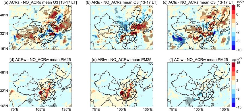
WRF-GC (v2.0): online two-way coupling of WRF (v3.9.1.1) and GEOS-Chem (v12.7.2) for modeling regional atmospheric chemistry-meteorology ...
←
→
Page content transcription
If your browser does not render page correctly, please read the page content below
Geosci. Model Dev., 14, 3741–3768, 2021
https://doi.org/10.5194/gmd-14-3741-2021
© Author(s) 2021. This work is distributed under
the Creative Commons Attribution 4.0 License.

WRF-GC (v2.0): online two-way coupling of WRF (v3.9.1.1) and
GEOS-Chem (v12.7.2) for modeling regional atmospheric
chemistry–meteorology interactions
Xu Feng1 , Haipeng Lin2 , Tzung-May Fu3,4 , Melissa P. Sulprizio2 , Jiawei Zhuang2 , Daniel J. Jacob2 , Heng Tian1 ,
Yaping Ma5 , Lijuan Zhang6 , Xiaolin Wang1 , Qi Chen7 , and Zhiwei Han8
1 Department  of Atmospheric and Oceanic Sciences, School of Physics, Peking University, Beijing, China
2 John  A. Paulson School of Engineering and Applied Sciences, Harvard University, Cambridge, MA, USA
3 State Environmental Protection Key Laboratory of Integrated Surface Water-Groundwater Pollution Control, School of

Environmental Science and Engineering, Southern University of Science and Technology, Shenzhen, Guangdong, China
4 Shenzhen Institute of Sustainable Development, Southern University of Science and Technology,

Shenzhen, Guangdong, China
5 National Meteorological Information Center, China Meteorological Administration, Beijing, China
6 Shanghai Central Meteorological Observatory, Shanghai, China
7 State Key Joint Laboratory of Environmental Simulation and Pollution Control, College of Environmental Sciences

and Engineering, Peking University, Beijing, China
8 Key Laboratory of Regional Climate-Environment for Temperate East Asia, Institute of Atmospheric Physics,

Chinese Academy of Sciences, Beijing, China

Correspondence: Tzung-May Fu (fuzm@sustech.edu.cn)

Received: 29 December 2020 – Discussion started: 8 February 2021
Revised: 10 May 2021 – Accepted: 25 May 2021 – Published: 23 June 2021

Abstract. We present the WRF-GC model v2.0, an on-               microphysics calculations. WRF-GC is computationally effi-
line two-way coupling of the Weather Research and Fore-          cient and scalable to massively parallel architectures. We use
casting (WRF) meteorological model (v3.9.1.1) and the            WRF-GC v2.0 to conduct sensitivity simulations with differ-
GEOS-Chem model (v12.7.2). WRF-GC v2.0 is built on the           ent combinations of ARI and ACI over China during January
modular framework of WRF-GC v1.0 and further includes            2015 and July 2016. Our sensitivity simulations show that in-
aerosol–radiation interaction (ARI) and aerosol–cloud inter-     cluding ARI and ACI improves the model’s performance in
action (ACI) based on bulk aerosol mass and composition,         simulating regional meteorology and air quality. WRF-GC
as well as the capability to nest multiple domains for high-     generally reproduces the magnitudes and spatial variability
resolution simulations. WRF-GC v2.0 is the first implemen-       of observed aerosol and cloud properties and surface meteo-
tation of the GEOS-Chem model in an open-source dynamic          rological variables over East Asia during January 2015 and
model with chemical feedbacks to meteorology. In WRF-            July 2016, although WRF-GC consistently shows a low bias
GC, meteorological and chemical calculations are performed       against observed aerosol optical depths over China. WRF-
on the exact same 3-D grid system; grid-scale advection of       GC simulations including both ARI and ACI reproduce the
meteorological variables and chemical species uses the same      observed surface concentrations of PM2.5 in January 2015
transport scheme and time steps to ensure mass conserva-         (normalized mean bias of −9.3 %, spatial correlation r of
tion. Prescribed size distributions are applied to the aerosol   0.77) and afternoon ozone in July 2016 (normalized mean
types simulated by GEOS-Chem to diagnose aerosol opti-           bias of 25.6 %, spatial correlation r of 0.56) over eastern
cal properties and activated cloud droplet numbers; the re-      China. WRF-GC v2.0 is open source and freely available
sults are passed to the WRF model for radiative and cloud        from http://wrf.geos-chem.org (last access: 20 June 2021).

Published by Copernicus Publications on behalf of the European Geosciences Union.
3742                        X. Feng et al.: WRF-GC v2.0: online two-way coupled regional meteorology–chemistry model

1   Introduction                                                     by offline meteorological data. As such, these stand-alone
                                                                     CTMs may be independently developed by a wider atmo-
Interactions between atmospheric constituents and meteoro-           spheric chemistry community, and the resulting CTM ad-
logical processes greatly impact regional weather and atmo-          vancement may be quickly incorporated into the coupled
spheric chemistry (Zhang, 2008; Baklanov et al., 2014). Me-          model via the online-access structure (Yu et al., 2014).
teorological conditions affect the emissions of chemical con-           Alternatively, regional coupled models may adopt an
stituents into the atmosphere from natural and anthropogenic         online-integrated structure, where the chemical module is
sources, as well as the subsequent chemical reactions, trans-        an internal component of the coupled model. This structure
port, and removal of those atmospheric constituents (Zhang           entails meteorological and chemical calculations being per-
et al., 2013; Zheng et al., 2015; Abel et al., 2017; Ma et al.,      formed on the same grids with the same time-stepping sys-
2020). In turn, atmospheric aerosols exert radiative forc-           tem. A major advantage of the online-integrated models is
ings either directly by scattering or absorption of radiation        that meteorological and chemical data do not need to be in-
(i.e., aerosol–radiation interaction, ARI), or indirectly by al-     terpolated in time or space for the coupling. Also, the trans-
tering the microphysical properties of clouds (i.e., aerosol–        port schemes for meteorological and chemical quantities are
cloud interaction, ACI) (Hansen et al., 1997; Haywood and            generally consistent in online-integrated models, which bet-
Boucher, 2000; Johnson et al., 2004; Lohmann and Feichter,           ter ensures mass conservation (Zhang, 2008). An example
2005). Many studies have demonstrated that in areas with             of the online-integrated coupled structure is the WRF-Chem
high aerosol concentrations, ARI and ACI can induce com-             model (Grell et al., 2005; Fast et al., 2006), which consists of
plex feedbacks to significantly affect both regional meteorol-       the WRF model and a chemical module; that chemical mod-
ogy and air quality (Li et al., 2007; Forkel et al., 2012; Ding      ule is called by WRF at each chemical time step. WRF-Chem
et al., 2013; J. Wang et al., 2014; Gong et al., 2015; Tao et al.,   includes options to turn on ARI and ACI, either individually
2015; Petaja et al., 2016; Z. Li et al., 2017; Zhao et al., 2017).   or combined. WRF-Chem has been widely used to study re-
We previously developed WRF-GC v1.0 (Lin et al., 2020),              gional air quality, meteorology, and their interactions (Zhang
an one-way online coupling of the Weather Research and               et al., 2010; Huang et al., 2016; Archer-Nicholls et al., 2016;
Forecasting (WRF) meteorological model (Skamarock et al.,            Zhang et al., 2018). However, the chemical module in WRF-
2008, 2019) and the GEOS-Chem model (Bey et al., 2001)               Chem cannot stand alone as a CTM.
for simulating regional air quality without aerosol feedbacks.          The WRF-GC model is developed using the online-
Here, we present the development of WRF-GC v2.0, which               integrated structure, with WRF calling the GEOS-Chem col-
further includes ARI, ACI, and nested-domain capabilities            umn model as an internal chemical module (Lin et al., 2020).
to better simulate interactions between regional meteorology         The exact same GEOS-Chem column model is also used by
and air quality at high resolution.                                  the GEOS-Chem “Classic” model to form a stand-alone of-
   The coupling between meteorological and chemical pro-             fline CTM, which has been actively developed by the at-
cesses in regional models is typically achieved by one of two        mospheric chemistry community (Bey et al., 2001; Eastham
methodologies: online-access coupling or online-integrated           et al., 2018). This architecture of the WRF-GC model is
coupling (Baklanov et al., 2014). Under the online-access            made possible by the recent “modularization” of the GEOS-
coupling framework, a meteorological model and a chemical            Chem model. GEOS-Chem was previously (before v11.01)
transport model (CTM) separately simulate regional meteo-            an offline CTM, driven by archived meteorological data
rology and atmospheric chemistry. At regular time intervals          at several static sets of global or regional 3-D grids, with
during runtime, they exchange meteorological and chemical            prescribed horizontal and vertical resolutions (Bey et al.,
data interpolated to the other model’s grids and time to drive       2001). Long et al. (2015) and Eastham et al. (2018) modular-
subsequent calculations. The meteorological model and the            ized the core chemical processes in GEOS-Chem, including
CTM may work with different 3-D grids, and they may use              emissions, chemistry, convective mixing, planetary boundary
different transport schemes for meteorological and chemi-            layer mixing, and deposition processes, to work in modular
cal variables. A number of two-way models are coupled us-            units of 1-D atmospheric vertical columns. Information about
ing the online-access approach, including, for example, the          the horizontal and vertical grids, formerly fixed at compile
online WRF – Community Multiscale Air Quality (WRF-                  time, is now passed to the GEOS-Chem column model at
CMAQ) model (Byun and Schere, 2006; Wong et al., 2012;               runtime (Long et al., 2015; Eastham et al., 2018; Lin et al.,
Yu et al., 2014), the Global Environmental Multiscale-Air            2020). This modularization allows the same GEOS-Chem
Quality model (GEM-AQ) (Kaminski et al., 2008), the Con-             chemical code to be either driven by offline meteorological
sortium for Small-Scale Modelling – Multiscale Chemistry             data (i.e., as a CTM) or be coupled online to dynamical mod-
Aerosol Transport (COSMO-MUSCAT) model (Wolke et al.,                els (Long et al., 2015; Eastham et al., 2018). To date, GEOS-
2004; Renner and Wolke, 2010), and the Integrated Fore-              Chem has been coupled to the NASA GEOS-5 Earth system
cast System-Model for Ozone And Related Tracers (IFS-                model (Hu et al., 2018), to the Beijing Climate Center atmo-
MOZART) model (Flemming et al., 2009). Often, the CTM                spheric general circulation model (Lu et al., 2020), and to
in online-access models can also stand alone and be driven

Geosci. Model Dev., 14, 3741–3768, 2021                                              https://doi.org/10.5194/gmd-14-3741-2021
X. Feng et al.: WRF-GC v2.0: online two-way coupled regional meteorology–chemistry model                                3743

the WRF regional meteorological model (Lin et al., 2020) in      sition, emissions, planetary boundary-layer mixing, gas and
distributed-memory frameworks for parallel computation.          aerosol chemistry, and wet scavenging (except advection), in
   WRF-GC v2.0 is the first implementation of the GEOS-          this order, within each atmospheric column at WRF-specified
Chem column model in an open-source dynamic model with           horizontal locations (Lin et al., 2020). Chemical information
chemical feedbacks to meteorology. WRF-GC v2.0 allows            is then passed back to WRF for the next time step. At the
GEOS-Chem users to investigate meteorology–atmospheric           end of the simulation, WRF finalizes the simulation and out-
chemistry interactions at a wide range of resolutions. WRF-      puts the meteorological and chemical outcomes. In WRF-
GC also offers other regional modellers access to the GEOS-      GC v1.0, the only chemistry-relevant operation performed
Chem chemical core, which is actively developed by a large       by WRF is the grid-scale advection of chemical species; the
user community and consistent with that in the GEOS-Chem         chemical species do not otherwise interact with the WRF
Classic offline CTM. WRF-GC v2.0 follows the modular             model.
coupling architecture of WRF-GC v1.0 (Sect. 2). In Sect. 3,         In WRF-GC v2.0, we implement ARI and ACI in the
we describe the development of ARI, ACI, and the nested-         two-way WRF-GC coupler. Figure 1a shows the two-
domain capability in WRF-GC v2.0. In Sect. 4, we assess          way WRF-GC coupler, which extends the capabilities
the performance of WRF-GC in simulating regional meteo-          of the one-way coupler by the addition of three mod-
rology and air quality against satellite and surface measure-    ules: (1) the Diag_Aero_Size_Info_Module,
ments. Finally, we assess the impacts of ARI and ACI on          (2)      the     optical_driver,           and     (3)    the
regional meteorology and chemistry in Sect. 5.                   mixactivate_driver. These three modules diag-
                                                                 nose the aerosol information from GEOS-Chem for the
                                                                 radiative transfer and cloud microphysics calculations
2     Overview of the WRF-GC two-way coupled model               in WRF. Figure 1b shows the workflow of the three
      architecture and its parent models                         new modules in WRF-GC v2.0. Users can switch on
                                                                 ARI or ACI by specifying aer_ra_feedback=1 or
2.1    Architecture of the WRF-GC two-way coupled                aer_cu_feedback=1, respectively, in the WRF-GC
       model                                                     configuration file (namelist.input). If ARI and ACI
                                                                 are both turned off, WRF-GC v2.0 will default to the
Figure 1 shows the architecture of the WRF-GC model,             one-way coupled simulation.
which consists of the two parent models (WRF and GEOS-              When users turn on the ARI, ACI, or both, the three
Chem) and a WRF-GC coupler that is completely indepen-           new modules are called by the WRF-to-chemistry interface
dent of both parent models. This architecture allows WRF-        (chem_driver) at the end of each chemical time step. The
GC to use native, unmodified versions of the parent models,      Diag_Aero_Size_Info_Module diagnoses the bulk
either one of which can be independently updated (Lin et al.,    aerosol mass information from GEOS-Chem (Sect. 2.2.1)
2020). In WRF-GC v1.0, the coupler consists of a state con-      and converts it into the sectional aerosol mass and num-
version module, a state management module, and the GEOS-         ber concentrations in specified size bins using prescribed
Chem column interface (Long et al., 2015; Eastham et al.,        size distributions (Sect. 3.1). The sectional aerosol infor-
2018; Lin et al., 2020). These modules manage the meteoro-       mation is then used by the optical_driver (Sect. 3.3)
logical and chemical information in distributed memory and       and by the mixactivate_driver (Sect. 3.4) to calcu-
perform state conversions between the two models at run-         late the aerosol and cloud optical properties and the ac-
time.                                                            tivated cloud droplet number concentrations, respectively.
   A WRF-GC simulation is initialized and managed by             The prognostic aerosol and cloud information is then passed
WRF, which sets the global clock, dynamical and chemi-           to the WRF model to be used by the radiative transfer
cal time steps, domain, horizontal resolution, and vertical      (module_radiation_driver) and cloud microphysics
coordinates, as well as initial/boundary conditions. In par-     (module_microphysics_driver) calculations at the
ticular, the 3-D grid system is determined by WRF and is         next time step. The diagnostic variables of aerosol mass and
fully adopted by the GEOS-Chem chemical module in units          number concentrations are added into the WRF-GC registry
of atmospheric columns. At each dynamical time step, WRF         file (registry.chem). Users can specify which variables
performs dynamical and physical calculations. WRF calcu-         to output in the registry file, and WRF will build the output
lates the grid-scale advection of meteorological variables and   arrays when WRF-GC is compiled. Below, we describe the
chemical species using the same transport scheme (Wicker         details of the WRF and GEOS-Chem models pertinent to the
and Skamarock, 2002), on the same grid system, and at the        two-way coupling. Further details on the two-way WRF-GC
same time steps, ensuring mass conservation of the chemical      coupler calculations are given in Sect. 3.
species. At each chemical time step, the meteorological and
chemical information is passed from WRF to GEOS-Chem
through the WRF-GC coupler. Then, the GEOS-Chem col-
umn model is called to perform convective mixing, dry depo-

https://doi.org/10.5194/gmd-14-3741-2021                                          Geosci. Model Dev., 14, 3741–3768, 2021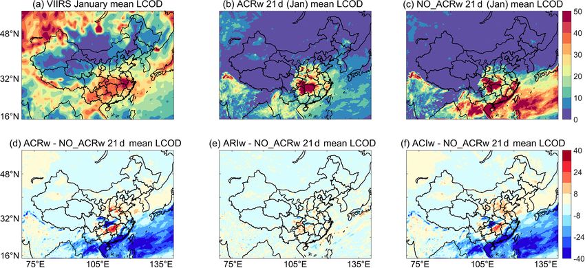
3744                        X. Feng et al.: WRF-GC v2.0: online two-way coupled regional meteorology–chemistry model

Figure 1. (a) Architectural overview of the WRF-GC coupled model (v2.0). The WRF-GC coupler (all parts shown in red) includes interfaces
to the two parent models, as well as the two-way coupling modules (shown in orange). The parent models (shown in gray) are standard codes
downloaded from their sources, without any modifications. (b) Flow diagram of the aerosol–radiation and aerosol–cloud interactions in the
WRF-GC coupled model (v2.0).

2.2     Parent models                                                  The standard chemical mechanism in GEOS-Chem v12.7.2
                                                                       includes a comprehensive Ox –NOx –VOC–halogen–aerosol
2.2.1    The GEOS-Chem model                                           chemical mechanism in the troposphere and uses the unified
                                                                       tropospheric–stratospheric chemistry extension (UCX) for
                                                                       stratospheric chemistry (Eastham et al., 2014). One of the
WRF-GC v2.0 currently uses GEOS-Chem v12.7.2
                                                                       critical updates in GEOS-Chem v12.7.2 is the reduced
(https://doi.org/10.5281/zenodo.3701669, The International
                                                                       sensitivity of surface resistance to temperature (Jaeglé
GEOS-Chem Community, 2020) as its chemical module, but
                                                                       et al., 2018). Also, the bulk surface resistance of nitric
users are also able to update to the latest standard version
                                                                       acid is updated to 1 s cm−1 to reflect its high affinity for
of GEOS-Chem through the existing WRF-GC architecture.
                                                                       natural surfaces. These updates increase the dry deposition
The chemical processes in GEOS-Chem v12.7.2 are mostly
                                                                       velocities of the nitric acid and nitrate, thereby correcting
the same as those in GEOS-Chem v12.2.1, which is used in
WRF-GC v1.0 and described in detail in Lin et al. (2020).

Geosci. Model Dev., 14, 3741–3768, 2021                                                 https://doi.org/10.5194/gmd-14-3741-2021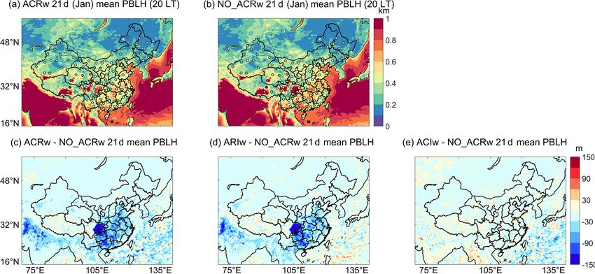
X. Feng et al.: WRF-GC v2.0: online two-way coupled regional meteorology–chemistry model                                     3745

previous overestimation of surface nitrate concentrations,        Aerosol Sectional (TOMAS) microphysics packages (Ko-
especially in winter (Jaeglé et al., 2018).                       dros and Pierce, 2017). These schemes more accurately sim-
   Aerosol species in the standard GEOS-Chem chemical             ulate size-dependent aerosol chemistry and microphysics, al-
mechanism include primary dust, sea salt, primary organic         beit at higher computational costs, but they are not yet sup-
carbon aerosol (POC), primary black carbon aerosol (BC),          ported by the GEOS-Chem column interface. Our developed
secondary inorganic aerosols (sulfate, nitrate, ammonium),        WRF-GC coupler with ARI and ACI can be extended to the
and secondary organic aerosols (SOAs) (Table 1). Sea salt         APM and TOMAS schemes in the future, once those two
aerosol masses in GEOS-Chem are simulated in two size             schemes become compatible with the GEOS-Chem column
ranges: the accumulation mode (dry radii between 0.1 and          interface.
0.5 µm) and the coarse mode (dry radii between 0.5 and 4 µm)
(Jaeglé et al., 2011). Dust aerosol masses are simulated in       2.2.2   The WRF model
four size ranges, with effective radii of 0.7, 1.4, 2.4, and
4.5 µm, respectively (Fairlie et al., 2007). All other aerosol    WRF-GC v2.0 currently uses the WRF model (v3.9.1.1) to
species are simulated by their individual bulk masses, assum-     perform online calculations of meteorological processes, ad-
ing static log-normal dry size distributions for each species     vection of chemical species, cloud microphysics, and ra-
(Martin et al., 2003; Drury et al., 2010; Jaeglé et al., 2011).   diative transfer with aerosol effects. WRF is a mesoscale
Secondary inorganic aerosols are simulated with the ISOR-         numerical weather model for research and operational ap-
ROPIA II algorithm (Fountoukis and Nenes, 2007). Freshly          plications (Skamarock et al., 2008, 2019). WRF simulates
emitted POC and BC aerosols are assumed to be 50 % hy-            atmospheric dynamics by solving fully compressible, Eu-
drophobic and 50 % hydrophilic, with a 1.2 d conversion           lerian non-hydrostatic equations on either hybrid sigma–
timescale from hydrophobic to hydrophilic (Q. Wang et al.,        eta (default) or terrain-following vertical coordinates. WRF
2014). Primary organic aerosol masses are estimated from          uses the staggered Arakawa C-horizontal grids at resolutions
POC mass using either a default global organic aerosol to or-     of 100 to 1 km and supports Lambert-conformal, Merca-
ganic carbon (OA / OC) mass ratio of 2.1 or spatiotemporally      tor, latitude–longitude, and polar stereographic projections.
varying OA / OC ratios (Philip et al., 2014). GEOS-Chem           WRF offers multiple parameterization options for cloud mi-
provides two options for simulating the formation of SOA.         crophysics, cumulus parameterization, planetary boundary
By default, GEOS-Chem uses the “simple SOA” scheme:               layer physics, shortwave/longwave radiative transfer, and
biogenic isoprene and monoterpene, as well as CO emitted          land surface physics (Skamarock et al., 2019). The options
from anthropogenic and biomass burning sources, are taken         currently supported in WRF-GC are listed in Lin et al.
as proxy precursors to irreversibly form SOA at specified         (2020).
mass yields on a 1 d timescale (Kim et al., 2015; Pai et al.,        Only a few radiative transfer and microphysics schemes
2020). This scheme simulates relatively accurate amounts          in WRF are currently coupled to prognostic aerosol infor-
of SOA without detailed chemical calculations (Miao et al.,       mation, and WRF-GC v2.0 supports these existing schemes.
2020). Alternatively, GEOS-Chem can also use a volatility         However, our treatments of aerosol information in the two-
basis set (VBS) scheme (Robinson et al., 2007; Pye et al.,        way WRF-GC coupler are abstracted and generalized, such
2010) to calculate complex SOA formation from the oxida-          that the coupler may be extended to support other radia-
tion of monoterpenes, sesquiterpenes, and light aromatics.        tive and microphysical schemes in WRF in the future. Most
The complex SOA scheme also includes SOA formed via               mesoscale simulations of ACI consider only the feedback
the aqueous-phase reactions of oxidation products from iso-       of aerosols to large-scale microphysics but do not explicitly
prene (Marais et al., 2016). GEOS-Chem assumes static, log-       simulate the impacts of aerosol on subgrid convective clouds
normal dry size distributions for its simulated bulk aerosol      (e.g., Wu et al., 2011; Zhao et al., 2017). Also, most of the cu-
species (except dust), as well as prescribed aerosol hygro-       mulus parameterization schemes in the standard WRF model
scopicity and optical properties at multiple wavelengths un-      (v3.9.1.1) do not respond explicitly to prognostic aerosol in-
der different relative humidity, for photolysis and hetero-       formation. The only exception is the Grell–Freitas ensemble
geneous chemistry calculations (Köpke et al., 1997; Martin        scheme (Grell and Freitas, 2014), which parameterizes the
et al., 2003; Drury et al., 2010; Jaeglé et al., 2011; Latimer    conversion of cloud water to rain water as a function of prog-
and Martin, 2019).                                                nostic cloud condensation nuclei (CCN) number. The Grell–
   In this work, we developed the two-way WRF-GC coupler          Freitas ensemble scheme will be supported in a future ver-
based on the standard bulk-mass representation of aerosol         sion of WRF-GC.
and the simple SOA scheme, involving the 14 aerosol types            In WRF, two shortwave radiation schemes are coupled to
shown in Table 1. The goal is to include the ARI and ACI in       prognostic aerosol information: the Rapid Radiative Trans-
WRF-GC while maintaining high computational efficiency.           fer Model for Global Circulation Model (RRTMG) short-
GEOS-Chem offers two optional schemes for size-resolved           wave radiation scheme (Iacono et al., 2008) and the Goddard
aerosol simulations: the Advanced Particle Microphysics           shortwave radiation scheme (Chou and Suarez, 1994). The
(APM) scheme (Yu and Luo, 2009) and the TwO-Moment                RRTMG shortwave radiation scheme includes atmospheric

https://doi.org/10.5194/gmd-14-3741-2021                                            Geosci. Model Dev., 14, 3741–3768, 2021
3746                        X. Feng et al.: WRF-GC v2.0: online two-way coupled regional meteorology–chemistry model

Table 1. Aerosol types in WRF-GC and their prescribed properties and size distributions.

       Name     Species                       Molecular      Density    Hygroscopicity            Log-normal             Log-normal
                                                 weight     (g cm−3 )        (unitless)           distribution            distribution
                                              (g mol−1 )                                     (geometric mean     (geometric standard
                                                                                            dry diameter, µm)     deviation, unitless)
       SO4      sulfate                               96          1.7               0.5                  0.14                     1.6
       NIT      nitrate                               62          1.8               0.5                  0.14                     1.6
       NH4      ammonium                              18          1.8               0.5                  0.14                     1.6
       OCPI     hydrophilic primary OC                12          1.3               0.2                  0.14                     1.6
       OCPO     hydrophobic primary OC                12          1.3               0.2                  0.14                     1.6
       BCPI     hydrophilic BC                        12          1.8      1.00 × 10⁻⁶                   0.04                     1.6
       BCPO     hydrophobic BC                        12          1.8      1.00 × 10⁻⁶                   0.04                     1.6
       SALA     accumulation-mode sea salt          31.4          2.2              1.16                  0.18                     1.5
                (radius 0.1–0.5 µm)
       SALC     coarse-mode sea salt                31.4          2.2              1.16                   0.8                     1.8
                (radius 0.5–4.0 µm)
       DST1     dust bin 1                            29          2.5              0.14                     –                       –
                (radius 0.1–1.0 µm)
       DST2     dust bin 2                            29        2.65               0.14                     –                       –
                (radius 1.0–1.8 µm)
       DST3     dust bin 3                            29        2.65               0.14                     –                       –
                (radius 1.8–3.0 µm)
       DST4     dust bin 4                            29        2.65               0.14                     –                       –
                (radius 3.0–6.0 µm)
       SOAS     SOA (simple)                         150          1.5              0.14                  0.14                     1.6

Rayleigh scattering, molecular absorption by water vapor,               ing the Ångström exponent method (Eck et al., 1999),
ozone, oxygen, carbon dioxide, and methane, as well as the              while the single scattering albedo (SSA) and the asym-
radiative extinction by clouds and aerosols in 14 spectral              metry factor are linearly interpolated. If ARI is turned
bands between 0.2 and 12.2 µm. The Goddard shortwave ra-                off (aer_ra_feedback=0 in namelist.input), the
diation scheme includes 11 spectral bands between 0.175 and             radiative schemes ignore the aerosol effects on radi-
10 µm. It calculates atmospheric Rayleigh scattering, absorp-           ation (aer_opt=0 in namelist.input), use cli-
tion by water vapor, ozone, oxygen, and carbon dioxide, as              matological aerosol data from Tegen et al. (1997)
well as scattering and absorption by clouds and aerosols. For           (aer_opt=1), or use the user-defined aerosol optical prop-
longwave radiation, only the RRTMG scheme (Iacono et al.,               erties (aer_opt=2) specified in the WRF-GC configuration
2008) has been coupled to prognostic aerosol information.               file (namelist.input).
The RRTMG longwave radiation scheme accounts for the                       For ACI, only two cloud microphysical schemes in the
absorption by water vapor, carbon dioxide, ozone, methane,              WRF model are coupled to prognostic aerosol informa-
oxygen, nitrous oxide, nitrogen, and several halocarbons, as            tion: the Lin et al. scheme (Lin et al., 1983; Chen and
well as cloud and aerosols.                                             Sun, 2002) and the Morrison two-moment scheme (Morri-
   When ARI is turned on (aer_ra_feedback=1 in                          son et al., 2009). WRF uses an aerosol activation scheme
namelist.input), WRF will ingest prognostic bulk                        developed by Abdul-Razzak and Ghan (2000, 2002). When
aerosol optical information from the interface with the                 ACI is turned on (progn=1 and naer=ignored in
chemistry module. WRF further interpolates the aerosol                  namelist.input), the interface to the chemical module
optical properties to the specific wavelengths compati-                 will call the aerosol activation scheme to diagnose the ac-
ble with the shortwave radiation schemes. The aerosol                   tivated cloud droplet number in a time step. This calcula-
optical depth (AOD) is interpolated or extrapolated us-                 tion is based on a maximum supersaturation determined by

Geosci. Model Dev., 14, 3741–3768, 2021                                                    https://doi.org/10.5194/gmd-14-3741-2021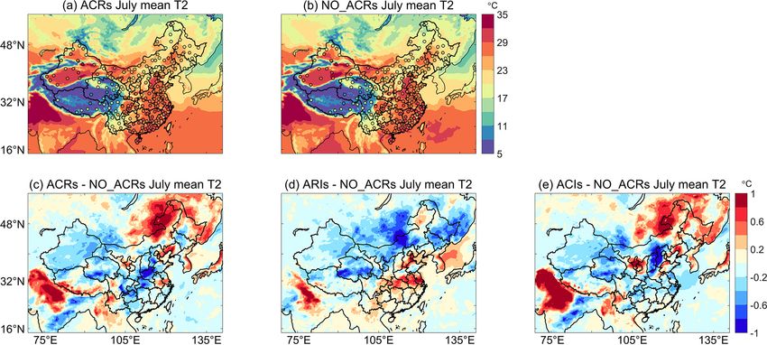
X. Feng et al.: WRF-GC v2.0: online two-way coupled regional meteorology–chemistry model                                        3747

the mass concentrations, number densities, and hygroscopic          Table 2. Upper and lower bounds of particle dry diameter for the
properties of aerosols, as well as the local air temperature and    four aerosol size bins used by WRF-GC.
updraft velocity. Also, the radiation module in WRF uses the
prognostic liquid cloud effective radii to compute the liquid                      Bin      Lower bound         Upper bound
cloud optical depths (LCODs). If ACI is turned off, WRF                                            (µm)                (µm)
either diagnoses the activated cloud droplet number using a                        1           0.0390625            0.15625
prescribed aerosol number and size distribution (progn=1                           2             0.15625              0.625
and naer=specified) or uses a constant source of acti-                             3                0.625               2.5
vated cloud droplets (100 cm−3 per time step in the Lin et                         4                  2.5              10.0
al. scheme and 250 cm−3 per time step in the Morrison two-
moment scheme) (progn=0). In the event where WRF does
use a constant source of activated cloud droplets, the pre-         is the number concentration density as a function of ln Di .
dicted cloud droplet number will effectively be around that         Dg,i and σi are the effective geometric mean dry diameter
prescribed number. Also, if ACI is turned off, WRF uses pre-        and the effective geometric standard deviation of the log-
scribed constant values of liquid cloud effective radii to cal-     normal distribution, respectively (Table 1). Thus, the mass
culate LCODs.                                                       concentration density of the ith aerosol type (mi (ln Di )) can
                                                                    be expressed using Di , ni (ln Di ), and the density of aerosol
3     New developments in WRF-GC v2.0                               type i (ρi ), as shown in Eq. (2):

Here, we describe the detailed diagnostics performed in                               π Di3
                                                                    mi (ln Di ) = ρi ·       · ni (ln Di )
the two-way WRF-GC coupler to communicate aerosol and                                   6
cloud information between GEOS-Chem and WRF. Some                                     π Di3
of our diagnostics are developed by imitating the connec-                      = ρi ·
                                                                                        6
tions between WRF and the chemical module in the WRF-                                             "                    2 #
                                                                                    N                  ln Di − ln Dg,i
Chem model (Grell et al., 2005; Fast et al., 2006; Chapman                     ·√           exp −                           .    (2)
et al., 2009). We also describe the software engineering de-                      2π ln σi                  2ln2 σi
velopments that enable nested-domain simulations in WRF-
GC v2.0.                                                               Table 1 summarizes the prescribed values of Dg,i , σi , and
                                                                    ρi for each aerosol type used in our two-way WRF-GC cou-
3.1    Diagnosing the size and number of dry aerosols               pler. The Dg,i and σi for secondary inorganic aerosols, BC,
                                                                    POC, and sea salt in accumulation and coarse modes are
The size distribution of aerosol is a critical prop-
                                                                    identical to the values used in the GEOS-Chem model for
erty that affects its optical effects and its abil-
                                                                    photolysis and heterogeneous chemistry calculations (Mar-
ity to be activated into CCN. We develop the
                                                                    tin et al., 2003; Drury et al., 2010; Jaeglé et al., 2011). We
Diag_Aero_Size_Info_Module to diagnose the
                                                                    assume that the log-normal distribution of SOA is identi-
sectional size distribution of aerosol mass and number
                                                                    cal to that of POC. The dry mass of aerosol type i (except
concentrations from the bulk aerosol masses simulated by
                                                                    dust) in each of WRF-GC’s four size bins can be calculated
GEOS-Chem. For each of the aerosol types (except dust)
                                                                    as Eq. (3):
in GEOS-Chem, we distribute the aerosol dry masses into
four effective dry diameter bins used by WRF-GC. We                               R hW,j
assume the aerosol within each size bin to be internally                           lW,j    mi (ln Di )d ln Di
                                                                    Mi,j = Mi · R ∞                             ,                (3)
mixed. The lower and upper dry diameter bounds of the four                          0     mi (ln Di )d ln Di
bins (Table 2) are from the Model for Simulating Aerosol
Interactions and Chemistry (MOSAIC) four-bin sectional              where lW,j and hW,j are the lower and upper dry diameter
parameterization (Zaveri et al., 2008). With the exception of       bounds of the j th size bin. Mi,j is the mass of aerosol type i
dust, we assume that the number density of aerosol type i           in the j th bin, and Mi is the total mass of aerosol type i. The
follows a log-normal distribution (Eq. 1):                          total number concentration of the internally mixed aerosol
                                                                    population (N ) cancels out in Eq. (3).
                  dN
ni (ln Di ) =                                                          GEOS-Chem simulates dust mass concentrations in four
                d ln Di                                             internal size bins, which need to be redistributed into the
                            "                      2 #
                    N            ln Di − ln Dg,i                    four size bins used by WRF and WRF-GC (shown in Ta-
          =√         exp −                                ,   (1)   ble 2). To achieve this, we mimic the redistribution scheme
            2π ln σi                  2ln2 σi
                                                                    of dust aerosols in the Goddard Chemistry Aerosol Radia-
where Di is the particle dry diameter, and N is the total num-      tion Transport model (GOCART, Chin et al., 2002), in which
ber concentration of the internally mixed particles. ni (ln Di )    the first four internal size bins are identical to those used in

https://doi.org/10.5194/gmd-14-3741-2021                                                  Geosci. Model Dev., 14, 3741–3768, 2021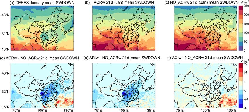
3748                         X. Feng et al.: WRF-GC v2.0: online two-way coupled regional meteorology–chemistry model

GEOS-Chem. In Eqs. (4) and (5), the l and h with the sub-           3.3   Aerosol–radiation interactions
scripts W and G represent the lower and upper dry diameter
bounds of each size bin used in WRF-GC and GEOS-Chem,               When ARI is turned on in WRF-GC v2.0,
respectively. The indices j and k refer to the size bins used       the new optical_driver module calls the
by WRF-GC and GEOS-Chem, respectively (j, k ∈ [1, 4]).              module_optical_averaging to diagnose the
Equation (4) calculates the fraction of dust mass within the        bulk optical properties of the internally mixed aerosols
GEOS-Chem size bin k that is mapped to the WRF-GC size              at each model grid and pass them to WRF for radiative
bin j . The mass is distributed by the logarithmic of parti-        transfer calculations. The diagnosed bulk optical properties
cle diameter. diag_dst(j ), the total dust mass concentrations      include the AOD, the SSA, and the asymmetry factor
within the WRF-GC size bin j , is the sum of the dust mass          at four specific wavelengths (300, 400, 600, 999 nm)
mapped into that bin from the four GEOS-Chem dust size              for shortwave radiative transfer and the AOD at 16 spe-
bins (Eq. 5).                                                       cific wavelengths for longwave radiative transfer. Our
                                                                 module_optical_averaging is developed by modi-
                max 0, min ln hW (j ), ln hG (k)                    fying a similar module from WRF-Chem (Fast et al., 2006).

                   −max ln lW (j ), ln lG (k)                       The module_optical_averaging module ingests
dstfrac(j, k) =                                            (4)
                       ln hG (k) − ln lG (k)                        the wet radius (Rw,j ) and the number concentration (Nj )
               X 4                                                  of aerosol particles in the j th size bin. The bulk refractive
diag_dst(j ) =     dst(k) · dstfrac(j, k) j, k ∈ [1, 4]    (5)      indices for the internally mixed aerosols in each size bin are
                k=1                                                 calculated by volume weighting the refractive indices for
   Equation (6) diagnoses the number concentrations of the          individual aerosol species using a look-up table (Barnard
internally mixed aerosols in eachP   size bin. The total dry        et al., 2010). The tabulated refractive indices for water,
aerosol volume in the j th size bin ( 10                            sulfate, dust, sea salt, and primary and secondary OC are
                                       i=1 Vd,i,j ) is calculated
by summing the dry aerosol volume of the 10 aerosol types.          wavelength dependent, while the refractive indices for other
The aerosol number concentrations in the j th size bin, Nj ,        aerosol species do not vary with wavelength. The module
can then be diagnosed by dividing the total dry aerosol vol-        then uses the bulk refractive indices to calculate the bulk
ume in that size bin by the mean particle size:                     extinction efficiency (Qe ), the bulk scattering efficiency
                                                                    (Qs ), and the intermediate asymmetry factor (g 0 ) for the
                    6              X10                              internally
                                                                              mixed
                                                                                    aerosols as a function of the size parameter
Nj =                          i3 ·     Vd,i,j .              (6)             2πR
         h
         1
                                                                    αj = λw,j based on Mie theory (Wiscombe, 1979). We
       π 2 (lW (j ) + hW (j ))     i=1
                                                                    use a Chebyshev economization (Press et al., 1992) to avoid
                                                                    the full Mie calculation at each time step following Fast
3.2    Diagnosing water uptake of aerosols
                                                                    et al. (2006). A full Mie calculation is only performed at the
The hygroscopic growth of aerosols at ambient relative hu-          first chemical time step to obtain the Chebyshev expansion
midity impacts their wet radii and optical properties. We           coefficients for each complex refractive index.
follow the method developed by Petters and Kreidenweis                 The bulk total extinction coefficient (bext ) at wavelength λ
(2007, 2013) to diagnose the uptake of water by aerosols and        is calculated as the sum of extinction by aerosols in all four
the resulting wet radii. According to the Zdanovskii–Stokes–        size bins (Eq. 9):
Robinson (ZSR) assumption (Stokes and Robinson, 1966),
the total aerosol liquid water is equal to the sum of the water                  4
                                                                                 X
                                                                                                      2
taken up by each aerosol constituent:                               bext (λ) =          Qe (αj ) · π Rw,j · Nj .                (9)
                                                                                 j =1
                 10
           aw X
Vw,j =              κi Vd,i,j .                              (7)
         1 − aw i=1                                                   The bulk AOD in a layer of atmosphere of dz thickness is
                                                                    (Eq. 10)
Vw,j is the total volume of aerosol liquid water in the j th
size bin. aw is the water activity, equal to the fractional rel-
ative humidity. κi is the hygroscopicity of the aerosol type        τ (λ) = bext (λ) · dz.                                     (10)
i (Table 1). The wet radius of the internally mixed aerosols
in the j th size bin, Rw,j , is required for the calculation of       The single scattering albedo ($0 ), which represents the
aerosol optical properties and are calculated by Eq. (8):           scattered percentage in the total light extinction of aerosol
                                !1                                  particles, is calculated as (Eq. 11)
         1 6 Vw,j + 10           3
                   P
                     i=1 Vd,i,j
Rw,j   =     ·                     .                         (8)
         2 π       Nj                                                             bs (λ)
                                                                    $0 (λ) =              ,                                    (11)
                                                                                 bext (λ)

Geosci. Model Dev., 14, 3741–3768, 2021                                                   https://doi.org/10.5194/gmd-14-3741-2021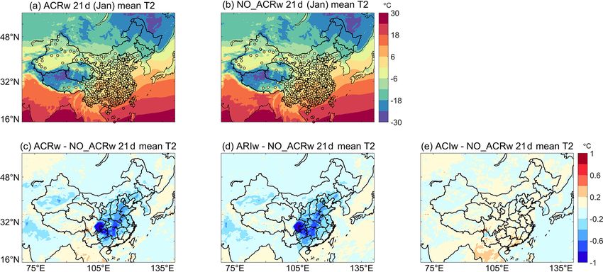
X. Feng et al.: WRF-GC v2.0: online two-way coupled regional meteorology–chemistry model                                   3749

where bs is the scattering coefficient of aerosols, given by
(Eq. 12)
           4
           X
                                2
bs (λ) =          Qs (αj ) · π Rw,j · Nj .                (12)
           j =1

  The bulk asymmetry factor, g, represents the asymmetry
between the forward scattering and backward scattering of
aerosol particles:
                                                                  Figure 2. Illustration of the WRF-GC state management module
           4                                                      operating in a nested-domain configuration.
                                2 · N · g 0 (α )
           P
                  Qs (αj ) · π Rw,j  j        j
           j =1
g(λ) =                                             ,      (13)
                            bs (λ)                                unactivated aerosols remain interstitial. The mixactivate
       g0
where is the intermediate asymmetry factor related to the         subroutine also calculates CCN at six specified supersatura-
size parameter αj .                                               tion ratios (0.02 %, 0.05 %, 0.1 %, 0.2 %, 0.5 %, and 1 %) as
                                                                  output diagnostics.
3.4   Aerosol–cloud interactions
                                                                  3.5   Development of nested-grid functionality and
We couple the activation of aerosol particles to the Mor-               online lightning NOx emissions
rison two-moment scheme (Morrison et al., 2009) and
the Lin et al. scheme (Lin et al., 1983; Chen and                 We implement the nested-domain functionality into WRF-
Sun, 2002) in WRF-GC. To achieve this, we develop                 GC v2.0 to enable meteorology–chemistry simulations at
an interface routine wrfgc_mixactivate (contained in              higher resolution. In WRF-GC v1.0 (Lin et al., 2020), the
module_mixactivate_wrappers in the coupler) by                    coupling between WRF and GEOS-Chem was limited to a
mimicking a similar routine in WRF-Chem. Equation (14)            single domain of arbitrary dimension and resolution. This
shows the rate of change of the cloud droplet number con-         was because the modules in previous GEOS-Chem versions
centration (Nc ) within a WRF model grid in the two cloud         (prior to v12.4.0) used a single memory space for the entire
microphysical schemes. The rate of change of Nc is deter-         simulation, such that the domain dimensions in GEOS-Chem
mined by the advection of cloud droplet number (−V ·∇Nc ),        were fixed once the simulation was initialized.
the vertical transport of cloud droplet number (D), the loss         We improve the state management module in WRF-
rate of cloud droplet number due to collision, coalescence,       GC v2.0 to better control the memory space of GEOS-Chem.
and collection (C), and the evaporation of cloud droplets (E),    Figure 2 illustrates the operation of the state management
as well as the rate of cloud droplet activation (S).              module when running WRF-GC v2.0 in a nested-domain
                                                                  configuration. When running a nested-domain simulation,
∂Nc
    = − (V · ∇Nc ) + D − C − E + S                        (14)    WRF designates separate memory space for each domain,
 ∂t                                                               and at each time step WRF alternately accesses the memory
   When ACI is turned on (aer_cu_feedback=1 and                   spaces for each domain. To achieve the same functionality
progn=1) in WRF-GC, the mixactivate_driver                        in GEOS-Chem, we modify the GEOS-Chem model (imple-
module in the WRF-GC coupler calls the existing WRF               mented in the standard code for v12.4.0 and after) so that
subroutine mixactivate through an interface routine               all of its internal variables are saved into state objects (me-
(wrfgc_mixactivate) to calculate the number of                    teorology, chemistry, and diagnostic state variables), which
aerosol particles activated into cloud droplets (S) and pass      are labeled for the specific simulation domain. We then mod-
it to WRF. wrfgc_mixactivate first calculates the                 ify the state management module, such that at each time
volume-weighted bulk hygroscopicity using the diagnostic          step during runtime, the state management module will de-
aerosol mass and number within each aerosol size bin and          termine the GEOS-Chem domain being processed, access
then calls the subroutine mixactivate. The subroutine             the corresponding state objects, and provide them to GEOS-
mixactivate uses the Köhler theory to calculate the acti-         Chem. The emission module of GEOS-Chem, the Harmo-
vated aerosol mass and number when the ambient supersatu-         nized Emissions Component (HEMCO), has also been up-
ration is over the critical supersaturation of aerosols (Abdul-   dated to fully objectify its memory space (Keller et al., 2014;
Razzak and Ghan, 2000, 2002). The total aerosol mass and          Lin et al., 2021). This allows WRF-GC v2.0 to execute sepa-
number concentrations are treated as two explicit population:     rate copies of HEMCO for each of the nested domains.
interstitial and cloud borne. The prognostic aerosol mass and        WRF-GC v2.0 allows both one-way and two-way infor-
number concentrations are initialized as interstitial before      mation exchange between the nested domains, supported by
passing to the mixactivate_driver module. The acti-               the WRF framework. In a nested-domain simulation, the
vated aerosols will be then considered cloud borne, while the     outer (coarser) domain will always provide lateral boundary

https://doi.org/10.5194/gmd-14-3741-2021                                            Geosci. Model Dev., 14, 3741–3768, 2021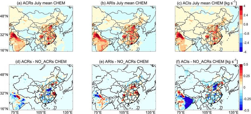
3750                       X. Feng et al.: WRF-GC v2.0: online two-way coupled regional meteorology–chemistry model

conditions to its immediate inner (finer) domain (one-way in-     expected, the slightly longer wall times in simulations with
formation exchange). Users may also turn on the two-way in-       chemical feedbacks are mostly associated with the extra cal-
formation exchange option (feedback=1 in the WRF-GC               culations within the WRF-GC coupler. The ARI calculations
namelist), which further allows information at the boundaries     incur more wall time increases than the ACI calculations do.
of the inner domain to be averaged and fed back to the im-        For reasons yet unclear, the wall time for the simulation with
mediate outer domain at every time step.                          ARI only (17 002 s) is slightly longer than that for the simu-
   In addition to the meteorology-dependent emissions in          lation with both ARI and ACI (16 153 s). Nevertheless, in all
WRF-GC v1.0 (Lin et al., 2020), in WRF-GC v2.0 we further         WRF-GC simulations, the coupling calculations are compu-
couple WRF meteorology to the online lightning NOx emis-          tationally economical and consume less than 9 % of the total
sion scheme in the HEMCO module (Murray et al., 2012).            wall times.
Intra-cloud and cloud-to-ground flash densities are functions
of the cloud-top height and are calculated by the lightning pa-
rameterization in WRF (Price and Rind, 1992; Wong et al.,         4     Validation of WRF-GC simulations of regional
2013). HEMCO then calculates lightning NOx emissions us-                meteorology and surface pollutant concentrations
ing the prescribed NOx production rates (500 moles per flash            over China
for latitudes northward of 35◦ N; 260 moles per flash else-
where) (Murray et al., 2012) and vertically distributes them      4.1    Setup of model experiments
from the surface to the local convective cloud-top level (Ott
et al., 2010).                                                    We next evaluate WRF-GC’s performance in simulating re-
                                                                  gional meteorology and surface pollutant concentrations.
3.6    Computational performance of WRF-GC v2.0                   We conduct two control simulations with full aerosol–
                                                                  cloud–radiation interactions using WRF-GC v2.0: one dur-
We conduct 2 d (27 to 29 June 2019) simulations using             ing January 2015 (Case ACRw) and one during July 2016
the WRF-GC (v2.0) model and the GEOS-Chem Clas-                   (Case ACRs). Table 4 summarizes the setup of our simu-
sic nested-grid model (v12.7.2) to compare their computa-         lations. Figure 3 shows our simulation domain over East
tional performance. Simulations with both models are con-         Asia, set by a Mercator projection at 27 km × 27 km spa-
figured with 245 × 181 atmospheric columns over China.            tial resolution. There are 50 vertical layers extending from
The WRF-GC simulations have 50 vertical levels, while the         the surface to 10 hPa. Case ACRw simulates 4 to 29 Jan-
GEOS-Chem Classic nested-grid simulation has 47 vertical          uary 2015; Case ACRs simulates 27 June to 31 July
levels. The WRF-GC model simulates meteorology online             2016. The first four days of each simulation initialize
(2 min dynamical time step), while the GEOS-Chem Classic          the model. Meteorological initial conditions and boundary
nested-grid simulation reads archived GEOS-FP assimilated         conditions (ICs/BCs) are taken from the National Centers
meteorological dataset (https://gmao.gsfc.nasa.gov/GMAO_          for Environmental Prediction (NCEP) Final (FNL) dataset
products/, last access: 20 June 2021) and calculates advection    (https://doi.org/10.5065/D6M043C6, National Centers for
at 5 min time step. All simulations use the same emissions,       Environmental Prediction et al., 2020) at 1◦ resolution.
the same chemical module (GEOS-Chem column model),                Chemical ICs/BCs are from a GEOS-Chem global simula-
and identical chemical time steps. All simulations are per-       tion at 2.5◦ longitude × 2◦ latitude, interpolated to WRF-GC
formed on the same single-node hardware with 24 Intel Cas-        horizontal and vertical grids. Meteorological and chemical
cade Lake physical cores, 100 GB of RAM, and a networked          BCs are updated every 6 h at the WRF-GC domain boundary.
Lustre high-performance file system. WRF-GC uses Mes-             The WRF-GC simulations are not nudged with meteorologi-
sage Passing Interface (MPI) parallelization, while GEOS-         cal observations.
Chem Classic uses OpenMP parallelization.                            We further conduct sensitivity simulations over China for
   Table 3 compares the simulation wall times for the WRF-        January 2015 and July 2016 with different combinations of
GC v2.0 model (with various chemical feedback options)            ARI and ACI to investigate the impacts of chemical feed-
and for the GEOS-Chem Classic nested-grid model. Simi-            backs on simulated meteorology and air quality (Table 4).
lar to our previous diagnosis (Lin et al., 2020), a one-way       The setups of these sensitivity simulations are identical to the
WRF-GC simulation (15 282 s) is 53 % faster than a simi-          control cases, except ARI and ACI are configured differently
larly configured GEOS-Chem Classic nested-grid simulation         in each sensitivity simulation (Table 4). In Cases NO_ACRs
(33 601 s). The better computational performance of WRF-          and NO_ACRw, both ARI and ACI are turned off, i.e., one-
GC is due to its faster dynamic calculations and its more ef-     way WRF-GC simulations with no chemical feedbacks to
ficient parallelization of the chemical processes (Lin et al.,    meteorology. Cases ARIs/ARIw and Cases ACIs/ACIw sim-
2020). The wall times for the two-way WRF-GC simulations          ulation include either ARI or ACI, respectively. Our simula-
with various combinations of chemical feedbacks (ARI only,        tions are conducted at a typical mesoscale resolution (27 km),
ACI only, and both ARI and ACI) are all less than 11 %            with the cumulus parameterization (new Tiedtke) and the
higher than the wall time for the one-way simulation. As          cloud microphysical scheme (Morrison two-moment) both

Geosci. Model Dev., 14, 3741–3768, 2021                                            https://doi.org/10.5194/gmd-14-3741-2021
X. Feng et al.: WRF-GC v2.0: online two-way coupled regional meteorology–chemistry model 3751
Table 3. Wall times of simulations conducted with the WRF-GC v2.0 model and the GEOS-Chem Classic nested-grid model (unit: s).
Model WRF-GC v2.0 GEOS-Chem Classic
Experiment One way ARI only ACI only ARI and ACI nested grid
v12.7.2
Total wall time 15 378 17 002 15 283 16 153 33 601
Breakdown: WRF 7766 8374 7274 7511 –
Breakdown: GEOS-Chem 7242 7242 7591 7206 –
Breakdown: WRF-GC coupler 370 1391 417 1436 –
Table 4. Configurations of WRF-GC v2.0 experiments in this study.
Experiment Case ACRs Case ARIs Case ACIs Case NO_ACRs
Simulation time 27 June 2016 00:00 Z to 31 July 2016 00:00 Z
Microphysics Morrison two-moment scheme (Morrison et al., 2009)
Shortwave radiation RRTMG (Iacono et al., 2008)
Longwave radiation RRTMG (Iacono et al., 2008)
Planetary boundary layer MYNN2 (Nakanishi and Niino, 2006)
Land surface Noah (Chen and Dudhia, 2001a, b)
Surface layer MM5 Monin–Obukhov (Jimenez et al., 2012)
Cumulus parameterization New Tiedtke (Tiedtke, 1989; C. Zhang et al., 2011; Zhang and Wang, 2017)
Aerosol–radiation interaction On On Off Off
Aerosol–cloud interaction On Off On Off
Experiment Case ACRw Case ARIw Case ACIw Case NO_ACRw
Simulation time 4 January 2015 00:00 Z to 29 January 2015 00:00 Z
Microphysics Morrison two-moment scheme (Morrison et al., 2009)
Shortwave radiation RRTMG (Iacono et al., 2008)
Longwave radiation RRTMG (Iacono et al., 2008)
Planetary boundary layer YSU (Hong et al., 2006)
Land surface Noah (Chen and Dudhia, 2001a, b)
Surface layer MM5 Monin-Obukhov (Jimenez et al., 2012)
Cumulus parameterization New Tiedtke (Tiedtke, 1989; C. Zhang et al., 2011; Zhang and Wang, 2017)
Aerosol–radiation interaction On On Off Off
Aerosol–cloud interaction On Off On Off
turned on. Thus, the subgrid convective clouds do not explic- 4.2 Observation datasets
itly respond to prognostic aerosol information. This setup is
typical of mesoscale simulations and has been shown to pro- 4.2.1 Satellite retrievals of AOD, cloud optical
duce similar aerosol sensitivities to those simulated at cloud- properties, and surface downward shortwave
resolving resolutions (Wu et al., 2011). radiation
Chinese monthly mean anthropogenic emissions are from
the Multi-resolution Emission Inventory for China (MEIC; We use satellite observations to evaluate WRF-GC’s per-
Li et al., 2014) with a resolution of 0.25◦ for the years formance in simulating aerosol and cloud optical proper-
2015 and 2016. Anthropogenic emissions from the rest of ties, and surface downward shortwave radiation. Monthly
Asia are from M. Li et al. (2017), developed for the year mean AOD observations are from the Deep Blue level-3
2010. Monthly mean biomass burning emissions are from the monthly aerosol products (AERDB_D3/M3_VIIRS_SNPP,
Global Emissions Database version 4 (GFED4; Randerson version 1) from the Visible Infrared Imaging Radiometer
et al., 2018). Meteorology-dependent emissions, including Suite (VIIRS) instruments at 1◦ spatial resolution (Sayer
the emissions of biogenic volatile organic compounds (Guen- et al., 2018). Monthly LCOD observations are from the
ther et al., 2012), sea salt (Gong, 2003), dust (Zender et al., VIIRS Cloud Properties level-3 monthly 1◦ grid products
2003), soil NOx (Hudman et al., 2012), and lightning NOx (CLDPROP_D3/M3_VIIRS_SNPP, version 1.1) (Platnick
(Murray et al., 2012), are calculated online in the HEMCO et al., 2019). Monthly surface downward shortwave radiation
module (Keller et al., 2014) in GEOS-Chem. observations for July 2016 are from the Earth Polychromatic
https://doi.org/10.5194/gmd-14-3741-2021 Geosci. Model Dev., 14, 3741–3768, 20213752 X. Feng et al.: WRF-GC v2.0: online two-way coupled regional meteorology–chemistry model
4.2.3 Surface measurements of air pollutants, air
temperature, and planetary boundary layer
height
Hourly surface measurements of PM2.5 and ozone are man-
aged by the Ministry of Ecology and Environment of China
(http://www.cnemc.cn, last access: 20 June 2021). Our pro-
tocol for data quality control follows Jiang et al. (2020). We
exclude sites with less than 90 % valid hourly data during
January 2015 and July 2016. For comparison between ob-
servations and model results, we calculate the average PM2.5
and ozone measurements in a WRF-GC grid. In all, we com-
pare model results to summertime ozone observations at 562
Figure 3. Spatial distributions of the observed and simulated time-
sites and to wintertime PM2.5 observations at 513 sites, re-
averaged AOD at 550 nm (a, c) during 8 to 28 January 2015 and
(b, d) during 1 to 30 July 2016. (a, b) Visible Infrared Imaging spectively. Surface air temperature measurements over China
Radiometer Suite (VIIRS) observations; (c) Case ACRw; (d) Case are downloaded from the US National Climate Data Center
ACRs. (https://gis.ncdc.noaa.gov/maps/ncei/cdo/hourly, last access:
20 June 2021), and we exclude sites with less than 90 % valid
data. In all, surface air temperature measurements at 150 and
Imaging Camera (EPIC)-derived products over land at 0.1◦ 215 sites are used to evaluate our simulations during January
resolution (Hao et al., 2020). The EPIC-derived total down- 2015 and July 2016, respectively. Finally, Guo et al. (2016)
ward shortwave radiation is consistent with the ground-based analyzed the rawinsonde observations over China to deter-
observations with a low global bias of −0.71 W m−2 over mine the daily planetary boundary layer heights (PBLHs)
land. For January 2015, due to the lack of EPIC-derived prod- during January 2011 to July 2015. We use the observed
ucts, we use the monthly gridded product from the Clouds PBLH at 120 sites at 08:00 and 20:00 local time (00:00 and
and the Earth’s Radiant Energy System (CERES) edition 4.1 12:00 UTC, respectively) to validate the simulated PBLH in
at 1◦ resolution (Rutan et al., 2015). The spatiotemporal vari- January 2015.
ations of the surface downward shortwave radiation observed
by the EPIC and CERES instruments are generally consistent 4.3 Validation of the simulated AOD over East Asia
(Hao et al., 2020).
Figure 3a and c compare the AOD at 550 nm wavelength over
4.2.2 Ground-based AOD measurements East Asia as observed by VIIRS and as simulated by WRF-
GC (Case ACRw) during 8 to 28 January 2015. For compari-
We evaluate the spectral AOD simulated by WRF-GC for
son against VIIRS observations, we use the simulated AODs
January 2015 against the ground-based observations from
at 300 and 999 nm to calculate the Ångström exponent of the
the Aerosol Robotic Network (AERONET, https://aeronet.
internally mixed bulk aerosol and then interpolated the sim-
gsfc.nasa.gov/, last access: 20 June 2021) project (version 3,
ulated AOD at 400 to 550 nm. WRF-GC is generally able to
level 2.0 quality-assured dataset, Giles et al., 2019). Hol-
reproduce the spatial distribution of AOD observed by VI-
ben et al. (1998) showed that the uncertainty of AERONET
IRS over eastern China (20–40◦ N, 105–130◦ E) with a spa-
AOD under cloud-free conditions was less than ±0.01 for
tial correlation coefficient of r = 0.64. WRF-GC reproduces
wavelengths over 440 nm. We select four representative sites
the high AOD values over the Sichuan Basin but underesti-
in eastern China, where there are more than 50 % valid ob-
mates the AOD over other parts of eastern China. The ob-
servations of spectral AOD at three wavelengths (500, 675,
served and simulated AODs at 550 nm over eastern China
and 1020 nm) during January 2015. These four sites are
in January 2015 are 0.37 and 0.21, respectively. WRF-GC
(1) Chinese Academy of Meteorological Sciences in Beijing
also underestimates the AOD over the Xinjiang, Qinghai, and
(39.93◦ N, 116.32◦ E), (2) Xianghe (39.75◦ N, 116.96◦ E),
Gansu provinces in western China, likely reflecting an under-
(3) China University of Mining and Technology in Xuzhou
estimation of dust.
(34.22◦ N, 117.14◦ E), and (4) Hong Kong Polytechnic Uni-
Figure 3b and d compare the observed and simulated (Case
versity in Hong Kong (22.30◦ N, 114.18◦ E).
ACRs) AOD at 550 nm during July 2016. VIIRS observes
AOD values exceeding 0.6 over the North China Plain (NCP)
area, reflecting the large amounts of aerosols and their hygro-
scopic growth over that area. The simulated spatial distribu-
tion of AOD is generally consistent with that from VIIRS, but
the peak values over the NCP are lower than the observations
by 50 %. We also compare model results to the AOD observa-
Geosci. Model Dev., 14, 3741–3768, 2021 https://doi.org/10.5194/gmd-14-3741-2021X. Feng et al.: WRF-GC v2.0: online two-way coupled regional meteorology–chemistry model 3753
tions from the MODIS instrument (Platnick et al., 2017a, b) central-western China, and along the southern slopes of the
and similarly find that the simulated AODs are spatially con- Himalayas. The observed and simulated LCODs are rela-
sistent but lower than the MODIS observations over eastern tively low over the Tibetan Plateau. The simulated domain-
China. average LCOD from Case ACRs is 12.0 ± 8.1, lower than
Figure 4 compares the time series of the simulated daily the domain-averaged LCOD retrieved by VIIRS (18.2 ± 7.5).
spectral AOD against the AERONET observations at the four The underestimation of simulated LCOD is mostly over
representative Chinese sites during 8 to 28 January 2015. western China and the South China Sea. Over eastern China
At each site, we interpolate the simulated spectral AODs at (eastward of 100◦ E), the simulated magnitude and spa-
400, 600, and 999 nm to the AERONET observation wave- tiotemporal patterns of LCOD are in good agreement with
lengths of 500, 675, and 1020 nm, respectively, using the the observations (spatial correlation coefficient of r = 0.64,
Ångström exponent method (Eck et al., 1999). WRF-GC re- normalized mean bias of −25.3 %). Figure 6a and b show
produces the observed day-to-day variation of AOD at these the observed and simulated (Case ACRw) average LCODs
four sites during January 2015. The temporal correlation co- during 8 to 28 January 2015. The model reproduces the spa-
efficients between the observed and simulated AODs at all tial distribution of LCODs observed by VIIRS over China,
sites and wavelengths range between 0.55 and 0.86, except including in particular the high LCODs over southern China.
for the correlation coefficient between the observed and sim- However, the simulated LCOD is considerably lower than the
ulated 500 nm AOD in Beijing (0.44). However, the sim- VIIRS LCOD observations elsewhere in the domain.
ulated AODs are consistently lower than the AERONET Figure 7 shows the monthly mean liquid cloud effective
AODs, especially during high AOD events. radii at cloud top from the Case ACRs simulation. Satellite
Our analyses above show that AODs simulated by WRF- retrievals of cloud effective radii often show large biases, ex-
GC reproduce the spatiotemporal variability of the AODs cept over areas dominated by liquid stratocumulus or stratus
observed by satellite and ground-based networks. However, clouds (Yan et al., 2015; Witte et al., 2018). We instead com-
the simulated AODs are consistently lower than these ob- pare the simulated liquid cloud effective radii to the reported
servations. Previous comparisons of AODs simulated by re- values from aircraft observations over China. The observed
gional models against satellite observations also often found effective radii of liquid cloud droplets over the NCP area
spatial consistency but significant low biases in the mod- in summer are in the range of 5.1 µm (±2.2 µm) to 6.3 µm
els (Gao et al., 2014; Gan et al., 2015; Xing et al., 2015; (±2.3 µm) (Deng et al., 2009; Q. Zhang et al., 2011; Zhao
Zhang et al., 2016). Curci et al. (2015) showed that the un- et al., 2018). Over southern China, the observed effective
certainties for the model AODs are associated with the as- radii of liquid cloud droplets in summer vary from 7.3 ± 1.7
sumed mixing state, refractive indices, and hygroscopicity to 7.9 ± 3.0 µm (Hao et al., 2017; Yang et al., 2020). Our
of aerosols. In particular, assumptions of the aerosol mixing simulated effective radii of liquid cloud droplets are consis-
state can lead to 30 % to 35 % uncertainty on the simulated tent with these observed sizes of liquid cloud droplets and
AOD (Fassi-Fihri et al., 1997; Curci et al., 2015). In addi- reflect the spatial difference between northern and southern
tion, the WRF-GC model may have underestimated the abun- China. The simulated mean effective radii are 8.4 ± 1.3 and
dance of aerosols over China, as indicated by the slight un- 10.7 ± 0.9 µm over the NCP and southern China in July 2016,
derestimation of surface PM2.5 concentrations shown below respectively.
(Sect. 4.6). On the other hand, several studies showed that
the regional distributions of AOD observed by VIIRS and 4.5 Validation of simulated regional surface
MODIS are consistent with the AERONET measurements, meteorology
but both VIIRS and MODIS observations are biased high
compared to AERONET observations over Asia (Wang et al., Figure 8a and b compare the surface downward shortwave ra-
2020). This high bias in the satellite-observed AOD may par- diation (SWDOWN) over East Asia from the EPIC-derived
tially account for the discrepancy between the simulated and observations and those simulated by WRF-GC (Case ACRs)
satellite AODs. The cause of the discrepancy between ob- in July 2016. The simulated spatial distribution of July mean
served and simulated AOD should be further investigated in SWDOWN is in good agreement with the EPIC-derived ob-
future studies. servations over East Asia, with a spatial correlation coef-
ficient of r = 0.73. The observed and simulated July mean
4.4 Validation of the simulated LCOD and liquid cloud SWDOWN over China are 288 ± 36 and 281 ± 48 W m−2 ,
droplet effective radii respectively, with a slight low bias of −2.4 % in the model.
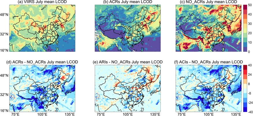
Figure 9a and b compare the mean SWDOWN observed by
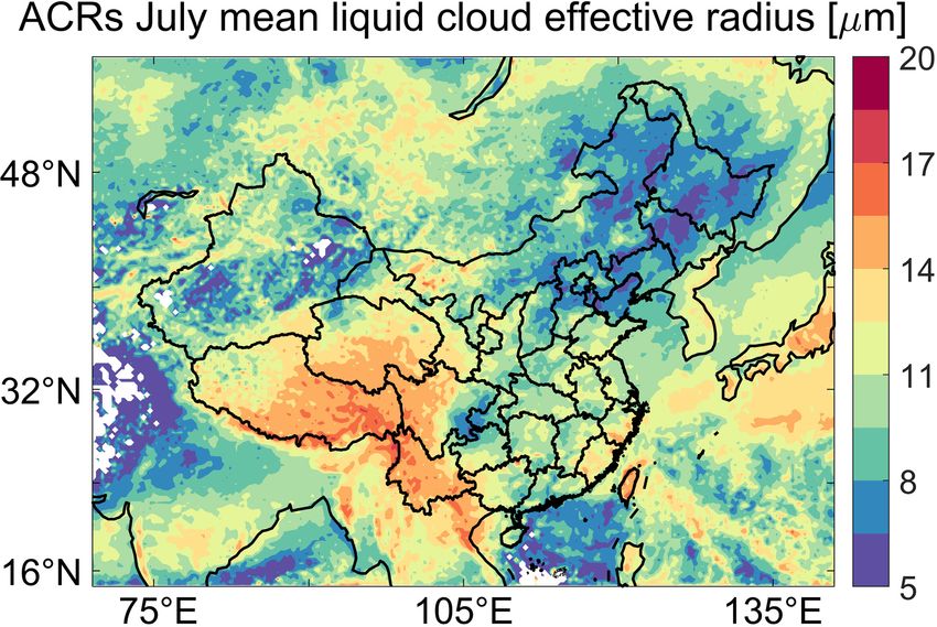
Figure 5a and b compare the July mean LCODs retrieved by CERES and that simulated by WRF-GC (Case ACRw) dur-
VIIRS and results from the Case ACRs simulation for July ing 8 to 28 January 2015. The spatial distribution of the sim-
2016. The spatial distributions of observed and simulated ulated wintertime SWDOWN also agrees well with the satel-
LCOD are generally consistent over East Asia. The observed lite observations, with a spatial correlation coefficient of 0.93
and simulated LCODs are both high over northeastern China, over the domain. The domain-average observed and simu-
https://doi.org/10.5194/gmd-14-3741-2021 Geosci. Model Dev., 14, 3741–3768, 2021You can also read