Long-term trends in air quality in major cities in the UK and India: a view from space
←
→
Page content transcription
If your browser does not render page correctly, please read the page content below
Atmos. Chem. Phys., 21, 6275–6296, 2021
https://doi.org/10.5194/acp-21-6275-2021
© Author(s) 2021. This work is distributed under
the Creative Commons Attribution 4.0 License.

Long-term trends in air quality in major cities in the UK and India:
a view from space
Karn Vohra1 , Eloise A. Marais2,a , Shannen Suckra1,b , Louisa Kramer1,c , William J. Bloss1 , Ravi Sahu3 ,
Abhishek Gaur3 , Sachchida N. Tripathi3 , Martin Van Damme4 , Lieven Clarisse4 , and Pierre-F. Coheur4
1 School of Geography, Earth and Environmental Sciences, University of Birmingham, Birmingham, UK
2 School of Physics and Astronomy, University of Leicester, Leicester, UK
3 Department of Civil Engineering, Indian Institute of Technology Kanpur, Kanpur, India
4 Université libre de Bruxelles (ULB), Spectroscopy, Quantum Chemistry and Atmospheric Remote Sensing (SQUARES),

Brussels, Belgium
a now at: Department of Geography, University of College London, London, UK
b now at: National Environment & Planning Agency, Kingston, Jamaica
c now at: Ricardo Energy & Environment, Harwell, UK

Correspondence: Eloise A. Marais (e.marais@ucl.ac.uk)

Received: 8 April 2020 – Discussion started: 26 August 2020
Revised: 11 March 2021 – Accepted: 12 March 2021 – Published: 29 April 2021

Abstract. Air quality networks in cities can be costly and        improvements there, despite the roll-out of controls on indus-
inconsistent and typically monitor a few pollutants. Space-       trial and transport sectors. Kanpur, identified by the WHO
based instruments provide global coverage spanning more           as the most polluted city in the world in 2018, experiences
than a decade to determine trends in air quality, augmenting      a significant and substantial (3.1 % a−1 ) increase in PM2.5 .
surface networks. Here we target cities in the UK (London         The decline of NO2 , NH3 , and PM2.5 in London and Birm-
and Birmingham) and India (Delhi and Kanpur) and use ob-          ingham is likely due in large part to emissions controls on
servations of nitrogen dioxide (NO2 ) from the Ozone Moni-        vehicles. Trends are significant only for NO2 and PM2.5 . Re-
toring Instrument (OMI), ammonia (NH3 ) from the Infrared         active NMVOCs decline in Birmingham, but the trend is not
Atmospheric Sounding Interferometer (IASI), formaldehyde          significant. There is a recent (2012–2018) steep (> 9 % a−1 )
(HCHO) from OMI as a proxy for non-methane volatile               increase in reactive NMVOCs in London. The cause for this
organic compounds (NMVOCs), and aerosol optical depth             rapid increase is uncertain but may reflect the increased con-
(AOD) from the Moderate Resolution Imaging Spectrora-             tribution of oxygenated volatile organic compounds (VOCs)
diometer (MODIS) for PM2.5 . We assess the skill of these         from household products, the food and beverage industry,
products at reproducing monthly variability in surface con-       and domestic wood burning, with implications for the for-
centrations of air pollutants where available. We find tem-       mation of ozone in a VOC-limited city.
poral consistency between column and surface NO2 in cities
in the UK and India (R = 0.5–0.7) and NH3 at two of three
rural sites in the UK (R = 0.5–0.7) but not between AOD
and surface PM2.5 (R < 0.4). MODIS AOD is consistent with         1   Introduction
AERONET at sites in the UK and India (R ≥ 0.8) and re-
produces a significant decline in surface PM2.5 in London         More than 55 % of people live in urban areas, and this is pro-
(2.7 % a−1 ) and Birmingham (3.7 % a−1 ) since 2009. We de-       jected to increase to 68 % by 2050 (UN, 2019). Air pollution
rive long-term trends in the four cities for 2005–2018 from       in cities routinely exceeds levels safe for human health (Lan-
OMI and MODIS and for 2008–2018 from IASI. Trends of              drigan et al., 2018). Regulatory air quality monitoring net-
all pollutants are positive in Delhi, suggesting no air quality   works, such as those employed in cities in the UK and India,
                                                                  provide detailed data concerning individual species and spe-

Published by Copernicus Publications on behalf of the European Geosciences Union.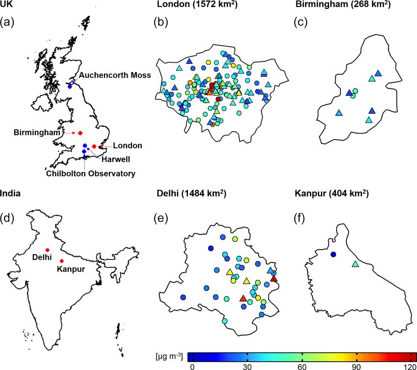
6276                                                           K. Vohra et al.: Long-term trends in air quality in major cities

cific locations but are labour-intensive to operate and main-       coal-fired power plants have been in place since December
tain, with potential gaps in spatial coverage and discontinu-       2015, but most power plants are non-compliant (Sugathan et
ities hindering longer term trend discovery. Here we assess         al., 2018). National PM2.5 concentration targets have been
the ability to use the long record of satellite observations        set at 20 %–30 % reductions by 2024 relative to 2017 levels
of atmospheric composition to monitor long-term trends in           (Govt. of India, 2019), but in 2016, measured annual mean
surface air quality in cities in the UK (London, Birming-           PM2.5 in Delhi and Kanpur exceeded the national standard
ham) and India (Delhi, Kanpur) of variable size, at a range         (40 µg m−3 ) by about a factor of 4 : 143 µg m−3 for Delhi and
of development stages, and with air pollutant concentrations        173 µg m−3 for Kanpur (WHO, 2018). In Delhi and Kanpur,
that pose a greater risk to health than previously thought          year-round emissions are dominated by vehicles, construc-
(Vodonos et al., 2018; Vohra et al., 2021).                         tion, and household biofuel use in the city and industrial ac-
   Our study focuses on two large cities in the UK (London          tivity and coal combustion nearby (Guttikunda and Jawahar,
and Birmingham) and two in India (Delhi and Kanpur). Each           2014; Venkataraman et al., 2018). Seasonal enhancements
is at a different stage of development: London is well devel-       come from intense agricultural fires along the Indo-Gangetic
oped, Birmingham is undergoing urban renewal, Delhi is ex-          Plain (IGP) north of Delhi, frequent firework festivals, and
periencing rapid development (Singh and Grover, 2015), and          dust storms originating from the Thar Desert and Arabian
Kanpur is a rapidly industrialising city (World Bank, 2014).        Peninsula (Ghosh et al., 2014; Parkhi et al., 2016; Yadav et
Air quality policy is well established in the UK, and the           al., 2017; Cusworth et al., 2018; Liu et al., 2018). Like the
rapid decline in regulated air pollutants and their precursors      UK, the agricultural sector is not directly regulated, and in-
has been monitored since 1970. According to the National            tense agricultural activity in the IGP contributes to the largest
Atmospheric Emission Inventory (NAEI), precursor emis-              global NH3 hotspot (Warner et al., 2017; Van Damme et al.,
sions of fine particles with aerodynamic diameter < 2.5 µm          2018; T. Wang et al., 2020).
(PM2.5 ) decreased in 1970–2017 by 1.5 % a−1 for nitrogen              Surface monitoring networks in cities in the UK and India
oxides (NOx ≡ NO + NO2 ), 2.0 % a−1 for sulfur dioxide              needed to evaluate citywide trends in air pollutant concentra-
(SO2 ), and 1.4 % a−1 for non-methane volatile organic com-         tions and precursor emissions can be exceedingly sparse and
pounds (NMVOCs). Primary PM2.5 emissions decreased by               are often short-term. To illustrate this, we show in Fig. 1 the
1.6 % a−1 over the same time period compared to a decline           coverage of surface sites in the four cities that continuously
of just 0.2 % a−1 for ammonia (NH3 ) emissions during 1980–         monitor NO2 , the most widely monitored air pollutant in both
2017 (Defra, 2019a). In UK cities, vehicles make a large con-       countries. There are also diffusion tubes and emerging tech-
tribution to air pollution year-round, with seasonal contribu-      nologies that measure NO2 at low cost, but these are suscep-
tions from residential fuelwood burning, agricultural activity,     tible to biases (Heal et al., 1999; Castell et al., 2017) and so
and construction and sporadic contributions from the long-          are excluded. The points in Fig. 1 show sites established and
range transport of Saharan dust (Fuller et al., 2014; Crilley et    maintained by national agencies, local city councils, and aca-
al., 2015; 2017; Harrison et al., 2018; Ots et al., 2018; Car-      demic institutions. These are coloured by multi-year mean
nell et al., 2019). Despite the decline in emissions, many ar-      NO2 around the satellite midday overpass (12:00–15:00 local
eas in the UK still exceed the legal annual mean limit of NO2       time or LT) for our period of interest (2005–2018). London
of 40 µg m−3 (Barnes et al., 2018), a threshold that may not        has the most extensive surface coverage. There can be more
adequately protect against the health effects of long-term ex-      than 100 sites operating simultaneously, but many of these
posure to NO2 (Lyons et al., 2020). Many areas will also ex-        are short-term. Most long-term sites are in central London,
ceed the annual mean PM2.5 standard, if updated from 25 to          and southeast London is devoid of stations. Birmingham has
10 µg m−3 , according to the WHO guideline (Defra, 2019b).          eight monitoring stations, but only two operated for the ma-
Reported annual mean PM2.5 in 2016, obtained as the surface         jority of 2005–2018. There are recently established compre-
monitoring network average, is 12 µg m−3 for London and             hensive air quality monitoring sites in London and Birming-
10 µg m−3 for Birmingham (WHO, 2018). There is increas-             ham, but these started operating in late 2018. More than 40 %
ing concern over emissions of the important PM2.5 precursor,        of the NO2 monitoring stations in Delhi were established in
NH3 , as there are no direct controls on the agricultural sec-      2018, and there are concerns over data access and quality
tor, the dominant NH3 source (Carnell et al., 2019). There has      (Cusworth et al., 2018). Fewer stations in the four cities mon-
even been a recent increase in NH3 emissions of 1.9 % a−1 in        itor PM2.5 than NO2 , and measurements of NMVOCs are
2013–2017 (Defra, 2019a), attributed to agriculture (Carnell        limited to a few short-term intensive campaigns and long-
et al., 2019).                                                      term sites that only measure light (short-chain) non-methane
   Air quality policy in India is in its infancy compared to        hydrocarbons. Long-term continuous monitoring of NH3 in
the UK. The first air pollution act was passed in 1981, 30          the UK is limited to hourly measurements at rural European
years after the equivalent in the UK. There has been a steady       Monitoring and Evaluation Programme (EMEP) sites (Fig. 1)
roll-out of European-style (Euro VI) vehicle emission stan-         and monthly measurements at UK Eutrophying and Acidify-
dards, starting with Delhi in 2018 and scaling up to the whole      ing Pollutants (UKEAP) network sites.
country by 2020 (Govt. of India, 2016). Strict controls on

Atmos. Chem. Phys., 21, 6275–6296, 2021                                               https://doi.org/10.5194/acp-21-6275-2021
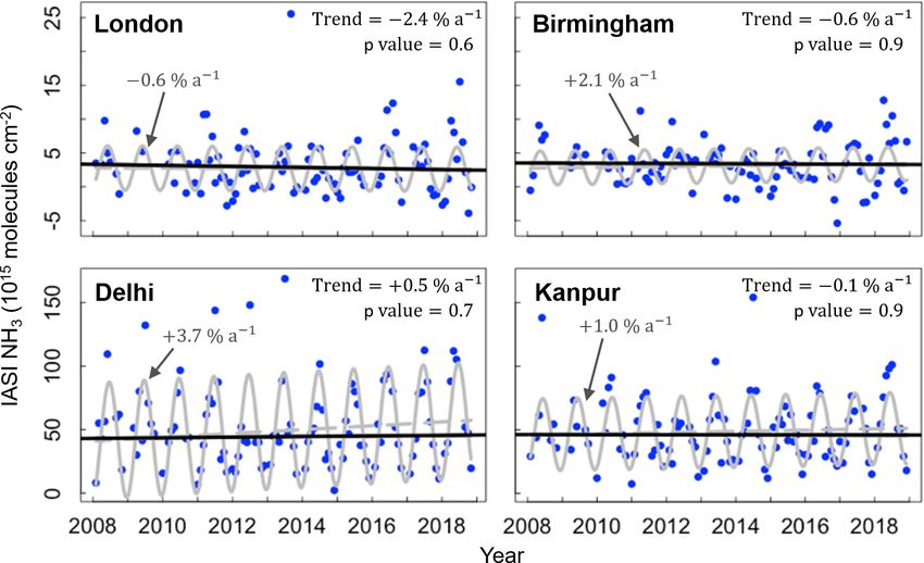
K. Vohra et al.: Long-term trends in air quality in major cities                                                                        6277

Figure 1. Spatial extent of surface NO2 monitoring stations in London (b), Birmingham (c), Delhi (e), and Kanpur (f). Panels (a) and (d)
show the location of the target cities (red) and UK sites that are part of the European Monitoring and Evaluation Programme (EMEP) (blue).
Panels (b), (c), (e), and (f) show the locations of local authority regulatory NO2 monitoring stations within the administrative boundaries of
each city, coloured by mean midday NO2 for 2005–2018 and separated into sites used (triangles) and not used (circles) to assess satellite
observations of NO2 (see text for details). The surface area of each city is indicated. Country and city boundaries are from GADM version
3.6 (GADM, 2018) and DataMeet (DataMeet, 2018).

   Satellite observations of atmospheric composition (Earth              produce the temporal variability of surface air pollution in
observations) provide consistent, long records (> 10 years)              the UK and India before going on to apply these satellite ob-
and global coverage of multiple air pollutants, complement-              servations to estimate long-term changes in air pollution to
ing surface monitoring networks with limited spatial cover-              assess the efficacy of air quality policies in the four cities of
age and temporal records (Streets et al., 2013; Duncan et al.,           interest.
2014). These have been used extensively as constraints on
temporal changes in surface concentrations of air pollutants
and precursor emissions (Kim et al., 2006; Lamsal et al.,                2    Space-based and surface air quality observations
2011; Zhu et al., 2014) but typically just targeting one–two
pollutants. In this work, we consider Earth observations of              Earth observations of NO2 and HCHO are from the Ozone
NO2 , formaldehyde (HCHO), NH3 , and aerosol optical depth               Monitoring Instrument (OMI), NH3 from the Infrared Atmo-
(AOD). HCHO is a prompt, high-yield, ubiquitous oxidation                spheric Sounding Interferometer (IASI), and AOD from the
product of NMVOCs used as a constraint on NMVOCs emis-                   Moderate Resolution Imaging Spectroradiometer (MODIS).
sions (Miller et al., 2008; De Smedt et al., 2010; Marais et al.,        There are also observations of SO2 and the secondary pol-
2012, 2014a, b). AOD has been used to derive surface con-                lutant ozone from OMI, but SO2 is below or close to the
centrations of PM2.5 for the global assessment of the impact             detection limit year-round for all cities, except in some
of air pollution on health (van Donkelaar et al., 2006, 2010,            months in Delhi, and UV measurements of tropospheric col-
Brauer et al., 2016; Anenberg et al., 2019).                             umn ozone have limited sensitivity to ozone in the bound-
   Here we conduct a systematic evaluation of the ability of             ary layer (Zoogman et al., 2011). TROPOspheric Monitor-
satellite observations of NO2 , NH3 , HCHO, and AOD to re-               ing Instrument (TROPOMI) sensitivity to SO2 is 4-fold bet-

https://doi.org/10.5194/acp-21-6275-2021                                                    Atmos. Chem. Phys., 21, 6275–6296, 2021
6278                                                           K. Vohra et al.: Long-term trends in air quality in major cities

ter than OMI, but the observation record is short (October          ary 2020). NASA AErosol RObotic NETwork (AERONET)
2017 launch) (Theys et al., 2019). We use hourly observa-           sun photometer AOD measurements (version 3.0, Level 2.0;
tions of NO2 and PM2.5 from the network of surface sites            https://aeronet.gsfc.nasa.gov/; last access: 5 February 2020)
in the four target cities and NH3 from the rural EMEP sites         are used to validate MODIS AOD at Chilbolton (UK) and
in the UK, to assess whether satellite observations of NO2 ,        Kanpur (India) (Holben et al., 1998; Giles et al., 2019).
AOD, and NH3 reproduce temporal variability of surface air
quality. There are no direct reliable measurements of HCHO          2.2   Earth observations of air pollution
in the UK, and measurements of NMVOCs are limited to a
few sites that only measure light (≤ C9) hydrocarbons.              OMI on board the NASA Aura satellite, launched in Octo-
   Figure 1 shows locations of EMEP sites in Harwell,               ber 2004, has a nadir spatial resolution of 13 km × 24 km
England, south of Oxford (51.57◦ N, 1.32◦ W), Chilbolton            and a swath width of 2600 km and passes overhead twice
Observatory, England, 65 km south of Harwell (51.15◦ N,             each day. OMI is a UV–visible spectrometer and so only
1.44◦ W), and Auchencorth Moss, Scotland, south of Edin-            provides daytime observations (13:30 LT). Global coverage
burgh (55.79◦ N, 3.24◦ W) (Malley et al., 2015, 2016; Walker        was daily in 2005–2009 and is every 2 d thereafter due to the
et al., 2019). Instruments at the Harwell site were relocated       row anomaly (http://omi.fmi.fi/anomaly.html, last access: 8
to Chilbolton Observatory in 2016, providing the opportunity        March 2020). We use the operational NASA OMI Level 2
to assess the satellite data at sites with distinct agricultural    product of tropospheric column NO2 for 2005–2018 (version
activity and anthropogenic influence (Walker et al., 2019).         3.0; https://doi.org/10.5067/Aura/OMI/DATA2017; last ac-
There are also passive NH3 samplers in the UK, but these            cess: 29 February 2020) (Krotkov et al., 2017). Total columns
have coarse temporal (monthly) resolution (Tang et al., 2018)       of HCHO are from the Quality Assurance for Essential Cli-
and no temporal correlation (R < 0.1) with a previous ver-          mate Variables (QA4ECV) OMI Level 2 product for 2005–
sion of the IASI NH3 product (Van Damme et al., 2015).              2018 (version 1.1; https://doi.org/10.18758/71021031; last
                                                                    access: 15 February 2020) (De Smedt et al., 2018). We re-
2.1    Surface monitoring networks in the UK and India              move OMI NO2 scenes with cloud radiance fraction ≥ 50 %,
                                                                    terrain reflectivity ≥ 30 %, and solar zenith angle (SZA) ≥
Surface sites in the UK with continuous (hourly) obser-             85◦ (Lamsal et al., 2010) and OMI HCHO scenes with pro-
vations of air pollutants typically use chemiluminescence           cessing errors and processing quality flags not equal to zero
instruments for NO2 , ion chromatography instruments for            (De Smedt et al., 2017). This removes scenes with cloud
NH3 (Stieger et al., 2018), and a range of reference in-            radiance fraction > 60 % and SZA > 80◦ . We apply addi-
struments for PM10 and PM2.5 . Sites used here in London            tional filtering to remove scenes with cloud radiance fraction
and Birmingham are from the national Department for En-             ≥ 50 % to be consistent with the threshold applied to OMI
vironment, Food and Rural Affairs (Defra) Automatic Ur-             NO2 . This additional filtering removes 16 % of the data for
ban and Rural Network (AURN) (https://uk-air.defra.gov.             London, 19 % for Birmingham, 7 % for Delhi, and 8 % for
uk/data/data_selector; last access: 28 January 2020) with           Kanpur.
additional sites in London from the King’s College Lon-                IASI on the polar sun-synchronous Metop-A satellite,
don Air Quality Network (LAQN) (https://www.londonair.              launched in October 2006, is an infrared instrument with
org.uk/london/asp/datadownload.asp; last access: 9 March            a morning (09:30 LT) and nighttime (21:30 LT) overpass. It
2019) and in Birmingham from Ricardo Energy & Environ-              provides global coverage twice a day with circular 12 km di-
ment (https://www.airqualityengland.co.uk/local-authority/          ameter pixels at nadir and a swath width of 2200 km. We use
data?la_id=407; last access: 24 January 2020) and Birm-             observations for the morning only, when the thermal contrast
ingham City Council. Observations at the UK EMEP sites              and sensitivity to the boundary layer are greatest (Clarisse et
are from the EMEP Chemical Coordinating Centre (http:               al., 2010; Van Damme et al., 2014). We use the Level 2 re-
//ebas.nilu.no/; last access: 9 March 2019). Measurements           analysis product of total column NH3 (version 3R) obtained
in India are limited to NO2 , PM10 , and PM2.5 monitoring           with consistent meteorology (ERA5) for clear-sky conditions
sites maintained in Delhi by the Central Pollution Control          (cloud fraction < 10 %) (Van Damme et al., 2020). The ear-
Board (CPCB), India Meteorological Department (IMD),                lier IASI NH3 product version (version 2R) was shown to be
and Delhi Pollution Control Committee (DPCC) and in Kan-            consistent with ground-based measurements of total column
pur by the Uttar Pradesh Pollution Control Board (UP-               NH3 at nine global sites (Dammers et al., 2016).
PCB) and the Indian Institute of Technology (IIT) Kan-                 The MODIS sensor on board NASA’s Aqua satellite,
pur (Gaur et al., 2014). PM2.5 measurements at IIT Kan-             launched in May 2002, has a swath width of 2330 km, crosses
pur form part of the international Surface Particulate Mat-         the Equator at 13:30 LT, and provides near-daily global cov-
ter Network (SPARTAN) (Snider et al., 2015; Weagle et al.,          erage. We use the Level 2 Collection 6.1 Dark Target daily
2018). Data from CPCB, IMD, DPCC, and UPPCB were                    AOD product at 550 nm and 3 km resolution (Remer et al.,
downloaded from the CPCB site (https://app.cpcbccr.com/             2013; Wei et al., 2019) (https://ladsweb.modaps.eosdis.nasa.
ccr/#/caaqm-dashboard/caaqm-landing; last access: 5 Febru-          gov/; last access: 29 February 2020). We use only the highest

Atmos. Chem. Phys., 21, 6275–6296, 2021                                              https://doi.org/10.5194/acp-21-6275-2021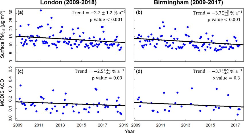
K. Vohra et al.: Long-term trends in air quality in major cities                                                            6279

quality AOD data (quality assurance flag of 3) (Munchak et         the sum of the reported NO and NO2 . We identify that NO2
al., 2013; Remer et al., 2013; Gupta et al., 2018).                reported in ppbv (29 % of DPCC, 10 % of CPCB and 74 %
                                                                   of UPPCB data) populates along the 1:1 line, and so we
                                                                   convert these data to µg m−3 using 1.88 µg m−3 ppbv−1 . The
3     Consistency between Earth observations and surface           same unit inconsistency does not exist for the IMD NO2 data.
      air pollution                                                These are reported throughout in ppbv and so are converted
                                                                   to µg m−3 .
Earth observation products retrieve column densities of pol-          We only consider surface observations coincident with
lutants throughout the atmospheric column (total for HCHO,         the OMI record (2005–2018), around the satellite overpass
AOD and NH3 ; troposphere for NO2 ) and are compared in            (12:00–15:00 LT). We find that NO2 declines at most sites in
what follows to surface concentrations from the surface mon-       London (ranging from −0.8 % a−1 to −3.6 % a−1 ) and Birm-
itoring network sites. This is to evaluate whether monthly         ingham (−1.1 % a−1 to −3.8 % a−1 ), with the exception of a
variability in the column reproduces variability in surface        few sites influenced by local sources. These include Maryle-
concentrations before going on to use the satellite observa-       bone Road in central London and Moor Street in Birming-
tions to quantify long-term trends in air pollution in the four    ham city centre. Both are impacted by dense traffic and de-
cities. The majority of the enhancement in the column, with        velopment projects (Carslaw et al., 2016; Harrison and Bed-
the exception of events like long-range transport, is near the     dows, 2017). We find that NO2 increases in Moor Street by
surface (Fishman et al., 2008; Duncan et al., 2014). Sources       6.8 % a−1 from 2013 to 2017. There are too few long-term
of errors in retrieval of HCHO and NO2 column densities            sites in Delhi and Kanpur to determine trends at individ-
include uncertainties in simulated vertical profiles and the       ual sites. We do not filter out sites based on site classifica-
presence of clouds and aerosols (Boersma et al., 2004; Lin         tion, as this information is not readily available for sites in
et al., 2015; Zhu et al., 2016; Silvern et al., 2018). Retrieval   India. Instead, we remove sites influenced by local effects
of NH3 column densities from IASI relies on thermal con-           and not consistent with month-to-month variability represen-
trast between the Earth’s surface and atmosphere and a suf-        tative of the city. This we do by detrending surface NO2 at
ficiently large training dataset (Whitburn et al., 2016; Van       each site, cross-correlating the detrended data for each site
Damme et al., 2017). Errors in retrieval of AOD include un-        and selecting sites with consistent month-to-month variabil-
certainties in aerosol properties and atmospheric conditions       ity (R > 0.5) in the detrended data. The original surface NO2
in matching simulated and observed top-of-atmosphere ra-           (including the trend) at the selected sites is then used to ob-
diances from single viewing angle instruments like MODIS           tain city-average monthly mean NO2 for comparison to OMI
(Remer et al., 2005; Levy et al., 2007, 2013). To the extent       NO2 .
that errors are random, these are reduced with temporal and           The selected sites are shown as triangles in Fig. 1. Filter-
spatial averaging.                                                 ing for spurious data and selection of consistent sites leads
   In what follows, city-average OMI NO2 and MODIS AOD             to 14 years of data at 46 sites in London, 5.5 years of data
are compared to representative city-average surface concen-        at 6 sites in Birmingham, and 8 years of data at 5 sites in
trations of NO2 in all four cities and PM2.5 in London and         Delhi. There are only 2 sites in Kanpur, but these are not
Birmingham. IASI NH3 is compared to coincident surface             consistent for the brief period of overlap (R < 0.5 for 2011–
observations of NH3 at UK EMEP sites (Fig. 1).                     2012), so we choose the site with the longest record (2011–
                                                                   2018). For the period of overlap for London and Birmingham
3.1    Assessment of OMI NO2                                       (2011–2016), mean city-average midday NO2 is 42.8 µg m−3
                                                                   for London and 26.5 µg m−3 for Birmingham. For Delhi
Data for NO2 in the UK include 152 monitoring sites in Lon-        and Kanpur (2011–2018 overlap), mean city-average midday
don, 8 in Birmingham, 37 in Delhi, and 2 in Kanpur (Fig. 1).       NO2 is 91.9 µg m−3 for Delhi and 48.4 µg m−3 for Kanpur.
The data we use for London and Birmingham have been                   We sample satellite observations within the administra-
independently ratified, but we still find and remove spuri-        tive boundaries of the four cities (Fig. 1) to capture the do-
ous NO2 observations. These include persistent (> 24 h) low        main that policymakers would target and assess. This is ex-
(< 1 µg m−3 ) values that do not exhibit diurnal variability.      tended a few kilometres beyond the administrative bound-
This occurs at fewer than 10 % of the sites and accounts           ary for Birmingham, as otherwise there are too few observa-
for at most 1 % of the data at these sites. We identified that     tions due to frequent clouds and small city size (∼ 300 km2 ).
NO2 data from DPCC and CPCB (Delhi) and from UPPCB                 Error-weighted OMI NO2 monthly means are estimated for
(Kanpur) networks are inconsistently reported in either parts      individual pixels centred within the administrative bound-
per billion by volume (ppbv) or micrograms per cubic metre         aries (including 6.5 km beyond for Birmingham). Months
(µg m−3 ). As information on the units of the individual data      with < five observations are removed. The number of months
is not provided, we determine whether NO2 is reported in           retained is 77 % for Birmingham, > 90 % for London, and
ppbv or µg m−3 by regressing total NOx (reported throughout        > 95 % for Delhi and Kanpur.
in ppbv, following the CPCB protocol; CPCB, 2015) against

https://doi.org/10.5194/acp-21-6275-2021                                            Atmos. Chem. Phys., 21, 6275–6296, 2021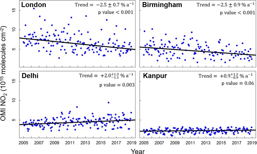
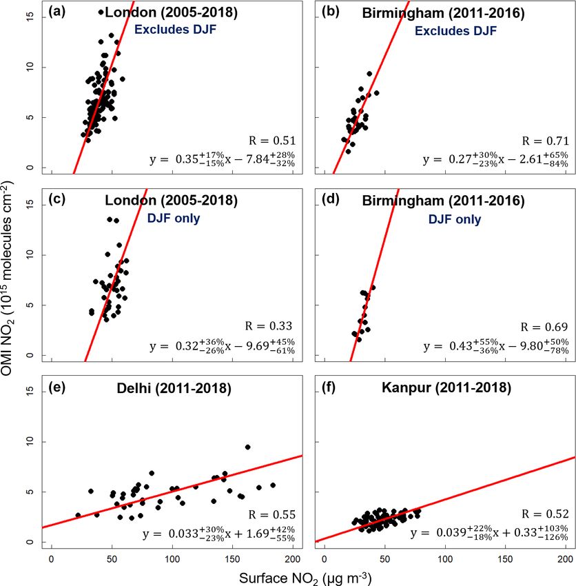
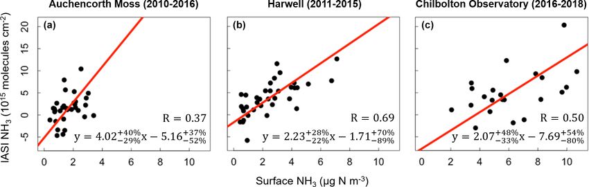
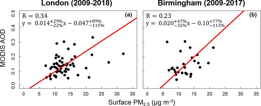
6280                                                           K. Vohra et al.: Long-term trends in air quality in major cities

   Figure 2 compares OMI and surface NO2 . The compar-              Delhi and Kanpur, this can lead to an ∼ 20 % underestimate
ison for London and Birmingham is divided into months               in OMI NO2 (Choi et al., 2020; Vasilkov et al., 2020).
excluding winter (December–February) and winter months
only. Factors that contribute to seasonality in the relation-       3.2   Assessment of IASI NH3
ship between tropospheric column and surface NO2 in loca-
tions with large seasonal shifts in temperature and solar in-       Figure 3 compares monthly mean IASI and surface NH3
solation include reduced photolysis rates, leading to longer        at the three UK EMEP sites. IASI is sampled up to
NOx lifetime in winter than summer (Boersma et al., 2009;           20 km around the surface site following the approach of
Kenagy et al., 2018; Shah et al., 2020) and a lower mixed           Dammers et al. (2016), and surface observations are sam-
layer height in winter than summer contributing to accumu-          pled around the IASI morning overpass (08:00–11:00 LT)
lation of pollution. Maximum mixed layer height for London          on days with coincident IASI observations. As with NO2 ,
is 900 m in winter compared to 1500 m in summer (Kotthaus           only months with more than five observations are used.
and Grimmond, 2018). The slope for Birmingham in win-               A total of 38 % of months are retained for Auchen-
ter (0.43 × 10¹⁵ molecules cm−2 (µg m−3 )−1 ) is steeper than       corth Moss, 62 % for Harwell, and 61 % for Chilbolton
that for non-winter months (0.27 × 10¹⁵ molecules cm−2              Observatory. For the months retained, average NH3 is
(µg m−3 )−1 ), but the difference is not significant. The sur-      1.6 µg nitrogen (N) m−3 for Auchencorth Moss, 2.5 µg N m−3
face NO2 measurements are also susceptible to interferences         for Harwell and 6.1 µg N m−3 for Chilbolton Observatory.
(positive biases) from thermal decomposition of NOx reser-          Chilbolton is southwest of mixed farmland, contributing to
voir compounds, such as peroxyacetyl nitrates in chemilumi-         levels of NH3 about 3 times higher than at Harwell (Walker
nescence instruments that use heated molybdenum catalysts           et al., 2019). Harwell has a more dynamic range in NH3
(Dunlea et al., 2007; Reed et al., 2016). The effect is worse       and stronger correlation (R = 0.69) than the other two sites
in winter than summer in London and Birmingham due to               (R = 0.37 for Auchencorth Moss; R = 0.50 for Chilbolton
the abundance of NOx reservoir compounds in winter (Lam-            Observatory). Weak correlation at Auchencorth Moss may
sal et al., 2010). OMI and surface NO2 monthly variability          be because surface NH3 concentrations are near the instru-
is consistent (R = 0.51–0.71), except for London in winter          ment detection limit (monthly mean NH3 < 2.0 µg N m−3 )
(R = 0.33). The correlation degrades (R = 0.40 for London,          and also because of low thermal contrast between the sur-
R = 0.54 for Birmingham) if all months are considered. The          face and overlying atmosphere (Van Damme et al., 2015;
seasonal dependence of the relationship between satellite and       Dammers et al., 2016). The slope for Auchencorth Moss
surface NO2 affects the ability to use OMI NO2 to infer sea-        (4.02 × 10¹⁵ molecules cm−2 (µg N m−3 )−1 ) is steeper than
sonality in the underlying NOx emissions. The same consis-          the slopes observed at sites with greater surface concen-
tency in monthly mean OMI and surface NO2 in non-winter             trations of NH3 (Harwell = 2.23 × 10¹⁵ molecules cm−2
months (R ≥ 0.6) has also been found over the UK city of Le-        (µg N m−3 )−1 and Chilbolton = 2.07 × 10¹⁵ molecules cm−2
icester (surface area 73 km2 ) (Kramer et al., 2008). Data for      (µg N m−3 )−1 ). Steeper slopes for sites with relatively low
all months are used for Delhi and Kanpur, as there is less vari-    NH3 concentrations are consistent with the assessment of
ability in mixed layer height in India than the UK. Seasonal        earlier IASI NH3 product versions (Van Damme et al., 2015;
mean maximum planetary boundary layer height in Delhi               Dammers et al., 2016).
varies from 1200 m in winter to 1400 m during monsoon
months (Nakoudi et al., 2019). Month-to-month variability           3.3   Assessment of MODIS AOD
in tropospheric column and surface NO2 (Fig. 2) is consis-
tent in Delhi (R = 0.55) and Kanpur (R = 0.52). OMI NO2             Figure 4 compares city-average monthly means of MODIS
exhibits much greater variability for an increment change           AOD and PM2.5 for London in 2009–2018 and for Birm-
in surface NO2 in the UK than in India, resulting in order-         ingham in 2009–2017. We use PM2.5 data from 24 sites in
of-magnitude lower slopes for Delhi and Kanpur (0.033               London and 8 sites in Birmingham. We add 2 more Birm-
and 0.039 × 10¹⁵ molecules cm−2 (µg m−3 )−1 ) than for Lon-         ingham sites by deriving PM2.5 from PM10 at 2 sites with
don and Birmingham (0.35 and 0.27 × 10¹⁵ molecules cm−2             only PM10 measurements. We use a conversion factor of
(µg m−3 )−1 ) (Fig. 2). This difference is likely due to a com-     0.85 (PM2.5 = 0.85× PM10 ) that we obtain from the slope of
bination of representativeness of surface sites and systematic      SMA regression of hourly PM2.5 and PM10 at 6 sites in Birm-
biases in the OMI NO2 retrieval. In Delhi, the proportion of        ingham with both measurements. We use a similar approach
sites used in Fig. 2 that measure the relatively lower con-         as applied to NO2 to assess AOD. Only surface observations
centration range of NO2 (annual mean NO2 < 50 µg m−3 ) is           around the satellite overpass (12:00–15:00 LT) and with con-
just 20 % compared to 74 % for London, leading to a posi-           sistent detrended month-to-month variability (R > 0.5) are
tive bias in city-average surface NO2 in Delhi. In Kanpur, we       retained to obtain citywide monthly mean PM2.5 . This results
use only one site located 600 m from a national motorway.           in 20 sites in London for 2009–2018 and 5 sites in Birming-
Aerosols are not explicitly accounted for in the OMI NO2            ham for 2009–2017. Mean midday city-average PM2.5 for
retrieval (Krotkov et al., 2017). For very polluted cities like     the period of overlap (2009–2017) is 13.7 µg m−3 in Lon-

Atmos. Chem. Phys., 21, 6275–6296, 2021                                              https://doi.org/10.5194/acp-21-6275-2021
K. Vohra et al.: Long-term trends in air quality in major cities                                                                         6281

Figure 2. Assessment of OMI NO2 with ground-based NO2 . Points are monthly means of city-average NO2 from OMI and the surface
networks for London (a, c), Birmingham (b, d), Delhi (e), and Kanpur (f). UK cities include panels with all months except December–
February (DJF) (a, b) and DJF only (c, d). Data for all months are given for cities in India. The red line is the standard major axis (SMA)
regression. Values inset are Pearson’s correlation coefficients and regression statistics. Relative errors on the slopes and intercepts are the
95 % confidence interval (CI).

Figure 3. Assessment of IASI NH3 with ground-based NH3 at UK EMEP sites. Points are monthly means from IASI and the surface
sites Auchencorth Moss (a), Harwell (b), and Chilbolton Observatory (c). The red line is the SMA regression. Values inset are Pearson’s
correlation coefficients and regression statistics. Relative errors on the slope and intercept are the 95 % CI. Locations of UK EMEP sites are
indicated in Fig. 1.

https://doi.org/10.5194/acp-21-6275-2021                                                    Atmos. Chem. Phys., 21, 6275–6296, 2021
6282                                                          K. Vohra et al.: Long-term trends in air quality in major cities

don and 11.3 µg m−3 in Birmingham. MODIS AOD monthly                  Figure 6 compares coincident AOD monthly means
means are estimated for London by averaging the pixels cen-        from MODIS and AERONET for Kanpur and Chilbolton.
tred within its administrative boundary and for Birmingham         Monthly variability in MODIS and AERONET AOD is con-
within and 6.5 km beyond the administrative boundary, as           sistent at both sites (R ≥ 0.8). MODIS exhibits no apprecia-
with OMI NO2 (Sect. 3.1). We remove months with < 160              ble bias at Kanpur. There is positive variance (slope = 1.4) at
observations, equivalent in spatial coverage to 5 OMI pix-         Chilbolton that may result from sensitivity to errors in sur-
els at nadir (the threshold used for OMI). After filtering,        face reflectivity at low AOD (Remer et al., 2013; Bilal et al.,
53 % of months are removed for London and 72 % for Birm-           2018) and residual cloud contamination (Wei et al., 2018,
ingham, mostly in winter. Fewer months than OMI are re-            2020). Mhawish et al. (2017) obtained similarly strong cor-
tained, as MODIS uses stricter cloud filtering. The correla-       relation (R = 0.8), but positive bias (26 %), of MODIS AOD
tions in Fig. 4 are weak (R = 0.34 for London, R = 0.23 for        at Kanpur from an earlier 3 km MODIS AOD product (Col-
Birmingham) and do not improve if we apply a less strict           lection 6).
threshold for the number of observations required to calcu-
late monthly means. The poor correlation may be due to
environmental factors that complicate the relationship be-         4   Air quality trends in London, Birmingham, Delhi,
tween AOD and surface PM2.5 , such as variability in mete-             and Kanpur
orological conditions, aerosol composition, enhancements in
                                                                   The consistency we find between satellite and ground-based
aerosols above the boundary layer, and the aerosol radiative
                                                                   monthly mean city-average NO2 (Fig. 2) and rural NH3
properties (Schaap et al., 2009; van Donkelaar et al., 2016;
                                                                   (Fig. 3) and trends in city-average PM2.5 (Fig. 5) supports
Shaddick et al., 2018; Sathe et al., 2019). We find that the
                                                                   the use of the satellite record to constrain surface air quality.
same assessment is not feasible for Delhi or Kanpur as the
                                                                   Variability in NO2 , HCHO, and NH3 columns can also be
record of surface PM2.5 and PM10 in these cities is too short.
                                                                   related to precursor emissions of NOx , NMVOCs, and NH3
   Figure 5 compares time series of monthly mean city-
                                                                   (Martin et al., 2003; Lamsal et al., 2011; Marais et al., 2012;
average MODIS AOD and surface PM2.5 in London (2009–
                                                                   Zhu et al., 2014; Dammers et al., 2019), as their lifetimes
2018) and Birmingham (2009–2017) to assess whether the
                                                                   against conversion to temporary or permanent sinks are rela-
weak correlation in Fig. 4 affects agreement in trends of the
                                                                   tively short, varying from 1–12 h depending on photochem-
two quantities. PM2.5 is longer lived than NO2 , so trends in
                                                                   ical activity, abundance of pre-existing acidic aerosols, and
PM2.5 (lifetime order weeks) for the limited number of sites
                                                                   proximity to large sources (Jones et al., 2009; Richter, 2009;
mostly located in central London should be more represen-
                                                                   Paulot et al., 2017; Van Damme et al., 2018). We adopt the
tative of variability across the city than the surface sites of
                                                                   same sampling approach as used to evaluate OMI NO2 . That
NO2 (lifetime order hours against conversion to temporary
                                                                   is, we sample the satellite observations within the city ad-
reservoirs). The steeper decline in surface PM2.5 in Birming-
                                                                   ministrative boundaries for London, Delhi, and Kanpur and
ham (3.7 % a−1 ) than in London (2.7 % a−1 ) is reproduced
                                                                   extend the sampling domain for Birmingham beyond the ad-
in the AOD record (3.7 % a−1 in Birmingham; 2.5 % a−1 in
                                                                   ministrative boundary by 6.5 km for OMI and MODIS and
London), although the AOD trends are not significant. In the
                                                                   10 km for IASI.
two UK cities, surface PM2.5 peaks in spring, whereas AOD
                                                                      We apply the Theil–Sen single median estimator to the
peaks in the summer, determined from multi-year monthly
                                                                   time series and also test the effect of fitting a non-linear func-
means (not shown). There are too few PM2.5 measurements
                                                                   tion (Weatherhead et al., 1998; van der A et al., 2006; Pope
in Delhi and Kanpur to compare long-term trends.
                                                                   et al., 2018) to account explicitly for seasonality:
   We compare the MODIS AOD product against ground-
truth AOD from AERONET at long-term sites in Kanpur and            Ym = A + BXm + C sin (ωXm + ∅) .                              (1)
Chilbolton to assess whether errors in satellite retrieval of
AOD contribute to the weak temporal correlation between            Ym is city-average satellite observations for month m, Xm is
MODIS AOD and surface PM2.5 . Daily AERONET AOD                    the number of months from the start month (January 2005 for
at 550 nm is estimated by interpolation using the second-          OMI and MODIS, and January 2008 for IASI), and A, B, C ,
order polynomial relationship between the logarithmic AOD          and ∅ are fit parameters. A is the city-average satellite ob-
and logarithmic wavelengths at 440, 500, 675, and 870 nm           servations in the start month, B is the linear trend, and
(Kaufman, 1993; Eck et al., 1999; Levy et al., 2010; Li et         [C sin (ωXm + ∅)] is the seasonal component that includes
al., 2012; Georgoulias et al., 2016). AERONET is sampled           the amplitude C, frequency ω (fixed to 12 months), and phase
30 min around the MODIS overpass, and MODIS is sampled             shift ∅. We only show the fit in Eq. (1) if the trend B is differ-
27.5 km around the AERONET site (Levy et al., 2010; Pe-            ent to that obtained with the Theil–Sen approach. The confi-
trenko et al., 2012; Georgoulias et al., 2016; McPhetres and       dence intervals (CIs) for the Theil–Sen trends are estimated
Aggarwal, 2018). Months with fewer than 160 MODIS ob-              using bootstrap resampling, and trends are considered signif-
servations are removed.                                            icant for p value < 0.05, that is, if the 95 % CI range does
                                                                   not intersect zero.

Atmos. Chem. Phys., 21, 6275–6296, 2021                                              https://doi.org/10.5194/acp-21-6275-2021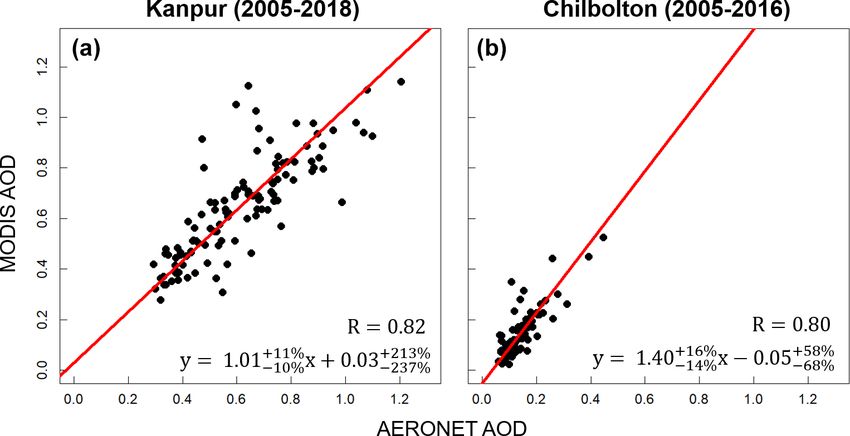
K. Vohra et al.: Long-term trends in air quality in major cities                                                                       6283

Figure 4. Assessment of MODIS AOD with surface PM2.5 in London (a) and Birmingham (b). Points are monthly means of city-average
AOD from MODIS and PM2.5 from surface networks for London and Birmingham. The red line is the SMA regression. Values inset are
Pearson’s correlation coefficients and regression statistics. Relative errors on the slopes and intercepts are the 95 % CI.

Figure 5. Time series of surface PM2.5 and MODIS AOD in 2009–2018 for London (a, c) and 2009–2017 for Birmingham (b, d). Points are
city-average monthly means of PM2.5 from the surface network (a, b) and AOD from MODIS (c, d). Black lines are trends obtained with
the Theil–Sen single median estimator. Values inset are annual trends and p values. Absolute errors on the trends are the 95 % CI. Trends are
considered significant at the 95 % CI (p value < 0.05).

   Figure 7 shows the time series of monthly means of                    seasonality for all cities (p value < 0.05 for the amplitude of
city-average OMI NO2 in the four cities for 2005–2018.                   the seasonality, C), but the linear trends are similar to those in
Decline in OMI NO2 in both London and Birmingham is                      Fig. 7: −2.4 % a−1 for London and Birmingham; unchanged
2.5 % a−1 and is significant. In Delhi, the OMI NO2 increase             for Delhi and Kanpur.
is 2.0 % a−1 and is significant (p value = 0.003), whereas the              Comparison of the OMI NO2 trends in Fig. 7 to surface
increase in Kanpur of 0.9 % a−1 is not (p value = 0.06). The             observations is only possible for London, where there are 46
relationship between tropospheric column and surface NO2                 sites with consistent month-to-month variability representa-
in London and Birmingham exhibits seasonality (Fig. 2).                  tive of the city that operated continuously from 2005 to 2018.
This is in part due to seasonality in mixing depth. We find              The trend obtained for OMI NO2 in London (−2.5 % a−1 )
that excluding the winter months in the time series has only             is steeper than we estimate with the surface monitoring sites
a small effect on the trend. NO2 should exhibit seasonality in           shown as triangles in Fig. 1 (1.8 % a−1 for 2005–2018). Most
all cities due to seasonal variability in its lifetime and sources       sites are in central London, and NO2 trends in outer London
(van der A et al., 2008). The fit in Eq. (1) yields significant          are 1.6 times steeper than in central London (Carslaw et al.,

https://doi.org/10.5194/acp-21-6275-2021                                                   Atmos. Chem. Phys., 21, 6275–6296, 2021
6284                                                              K. Vohra et al.: Long-term trends in air quality in major cities

Figure 6. Validation of MODIS AOD with AERONET AOD in Kanpur and Chilbolton. Points are monthly means of MODIS and AERONET
AOD for Kanpur (a) and Chilbolton (b). The red line is the SMA regression. Values inset are Pearson’s correlation coefficients and regression
statistics. Relative errors on the slopes and intercepts are the 95 % CI.

Figure 7. Time series of OMI NO2 in 2005–2018 for London, Birmingham, Delhi, and Kanpur. Points are city-average monthly means.
Black lines are trends obtained with the Theil–Sen single median estimator. Values inset are annual trends and p values. Absolute errors on
the trends are the 95 % CI.

2011). The decline in NO2 in the two UK cities is less than              is also weakened sensitivity of the tropospheric column to
the rate of decline in national NOx emissions (3.8 % a−1 )               changes in surface NO2 due to a gradual increase in the rel-
for 2005–2017 from the national bottom-up emission inven-                ative contribution of the free tropospheric background to the
tory (Defra, 2019a). This may reflect a combination of fac-              tropospheric column (Silvern et al., 2019). This weakening
tors. There is less steep decline in NOx emissions in Lon-               of the trend in the tropospheric column will likely be less
don compared to the national total that may in part be due to            in London than in Birmingham, due to greater local surface
discrepancies between real-world and reported diesel NOx                 emissions in large cities such as London (Zara et al., 2021).
emissions (Fontaras et al., 2014), sustained heavy traffic in            The positive trends in Delhi and Kanpur likely reflect a 2-
central London, and an increase in NO2 -to-NOx emission ra-              fold increase in vehicle ownership in Delhi (Govt. of Delhi,
tios dampening decline in NO2 (Grange et al., 2017). There               2019), rapid industrialisation in Kanpur (Nagar et al., 2019),

Atmos. Chem. Phys., 21, 6275–6296, 2021                                                     https://doi.org/10.5194/acp-21-6275-2021
K. Vohra et al.: Long-term trends in air quality in major cities                                                             6285

and the limited effect of air quality policies on pollution         Similar to NO2 , all four cities show significant seasonality
sources. This is corroborated by NOx emissions compliance           (p value < 0.05 for the amplitude of the seasonality, C). The
failures at more than 50 % of coal-fired power plants in Delhi      linear trends (dashed grey lines in Fig. 8) are more positive
and the surrounding area (Pathania et al., 2018). The lack of       than those obtained with Theil–Sen for all four cities but are
trend reversal in Delhi, despite implementation of air quality      still not significant. This leads to a trend reversal in Kan-
policies, is consistent with the lack of trend reversal reported    pur (+1.0 % a−1 ) and Birmingham (+2.1 % a−1 ), steeper in-
by Georgoulias et al. (2019). They used a 21-year record            crease in Delhi (+3.7 % a−1 ), and a less negative trend in
(1996–2017) of multiple space-based sensors to estimate a           London (−0.6 % a−1 ).
significant and sustained increase in NO2 of 3.1 % a−1 in              Relating trends in NH3 columns to trends in NH3
Delhi. By the end of 2018, tropospheric column NO2 is simi-         emissions is complicated by partitioning of NH3 to
lar in London and Delhi (5.7 × 10¹⁵ molecules cm−2 ; Fig. 7),       aerosols to form ammonium and dependence of this pro-
but OMI NO2 over India may be biased low, due to the pres-          cess on pre-existing aerosols that have declined in abun-
ence of optically thick aerosols (AOD > 0.4; Fig. 6) that are       dance across the UK due largely to controls on pre-
not explicitly accounted for in the retrieval (Sect. 3.1).          cursor emissions of SO2 (Vieno et al., 2014). Harwell
   The direction of the trends for all four cities is con-          and Auchencorth Moss include measurements of gas-phase
sistent with other trend studies, with differences in the           NH3 and aerosol-phase ammonium in PM2.5 . These ex-
absolute size of the trend due to differences in instru-            hibit large and distinct seasonality, so we use Eq. (1)
ments, time periods, and sampling domains. Pope et                  to estimate changes of −0.096 µg N m−3 a−1 for ammo-
al. (2018) observed declines in OMI NO2 for 2005–2015 of            nium and +0.031 µg N m−3 a−1 for NH3 at Auchencorth
2.3 ± 0.5 × 10¹⁴ molecules cm−2 a−1 for London and 1.1 ±            Moss in 2008–2012 and similar changes at Harwell in
0.5 × 10¹⁴ molecules cm−2 a−1 for Birmingham. We obtain a           2012–2015 of −0.10 µg N m−3 a−1 for ammonium and
similar trend for Birmingham but a steeper decline for Lon-         +0.035 µg N m−3 a−1 for NH3 . Only the decline in ammo-
don of 2.6 × 10¹⁴ molecules cm−2 a−1 using our sampling             nium at Auchencorth Moss is significant. This suggests the
domain for 2005–2015, though the difference is not signif-          increase in rural NH3 includes contributions from unregu-
icant. Schneider et al. (2015) obtained less steep and non-         lated agricultural emissions and reduced partitioning of NH3
significant changes in NO2 in London (−1.7 ± 1.2 % a−1 )            to pre-existing aerosols. The opposite trend (decline) in NH3
and Delhi (1.4 ± 1.2 % a−1 ) from the SCanning Imaging              in London obtained with Theil–Sen and Eq. (1) (Fig. 8) may
Absorption spectroMeter for Atmospheric CHartographY                be because decline in local vehicular emissions of NH3 with
(SCIAMACHY) for 2002–2013. Trends in OMI NO2 for                    a shift in catalytic converter technology (Richmond et al.,
2005–2014 from ul-Haq et al. (2015) are similar to ours for         2020) outweighs the increase in NH3 from waste and domes-
Delhi (2.0 % a−1 ) but lower for Kanpur (0.2 % a−1 ). Stud-         tic combustion (Defra, 2019a), and nearby agriculture (Vieno
ies have also combined multiple instruments to derive trends        et al., 2016) and offsets reduced partitioning of NH3 to acidic
since the mid-1990s. These find decreases in NO2 over Lon-          aerosols with decline in sulfate. The opposite effect would be
don of 0.7 % a−1 for 1996–2006 (van der A et al., 2008)             expected in Delhi due to nationwide increases in SO2 emis-
and 1.7 % a−1 for a longer observing period (1996–2011)             sions and sulfate abundance (Klimont et al., 2013; Aas et
(Hilboll et al., 2013) and a consistent increase for Delhi of       al., 2019). That is, the increase in NH3 emissions may be
7.4 % a−1 in 1996–2006 (van der A et al., 2008) and 1996–           steeper than the increase in NH3 columns in Fig. 8 due to a
2011 (Hilboll et al., 2013), much steeper than ours in Fig. 7.      corresponding increase in partitioning of NH3 to pre-existing
   Figure 8 shows time series of monthly means of city-             aerosols as these become more abundant.
average IASI NH3 in the four cities for 2008–2018. Mean                Figure 9 shows the time series of city-average monthly
IASI NH3 is 15–20 times more in Delhi and Kanpur than               mean OMI HCHO for the four cities for 2005–2018 af-
in London and Birmingham due to larger emissions of NH3             ter removing the background contribution from oxidation of
in the IGP, higher ambient temperatures promoting volatil-          methane and other long-lived volatile organic compounds
isation of NH3 , and greater sensitivity of IASI to NH3 due         (VOCs) to isolate variability in the column due to reac-
to greater thermal contrast between the surface and the at-         tive NMVOCs (Zhu et al., 2016). A representative back-
mosphere over India (Van Damme et al., 2015; Dammers                ground is obtained as monthly mean OMI HCHO over the
et al., 2016; T. Wang et al., 2020). IASI NH3 decreases             remote Atlantic Ocean (25–35◦ N, 35–45◦ W) for the UK
by 0.1 % a−1 in Kanpur, 0.6 % a−1 in Birmingham, and                and the remote Indian Ocean (10–20◦ S, 70–80◦ E) for In-
2.4 % a−1 in London and increases by 0.5 % a−1 in Delhi.            dia. The non-linear function in Eq. (1) is fit to these back-
None of the trends are significant. Measurements of surface         ground HCHO values and used to subtract the background
NH3 from continuous monitors deployed in Delhi in April             contribution, as in Marais et al. (2012), from the city-average
2010 to July 2011 exhibit the same seasonality as IASI NH3 ,        monthly means. OMI HCHO columns from oxidation of re-
peaking in the monsoon season (July–September) (Singh and           active NMVOCs in Delhi and Kanpur are almost twice those
Kulshrestha, 2012). We investigated the effect of NH3 sea-          in London and Birmingham due to a combination of unreg-
sonality on the trend using Eq. (1) (solid grey lines in Fig. 8).   ulated sources (Venkataraman et al., 2018) and high temper-

https://doi.org/10.5194/acp-21-6275-2021                                             Atmos. Chem. Phys., 21, 6275–6296, 2021
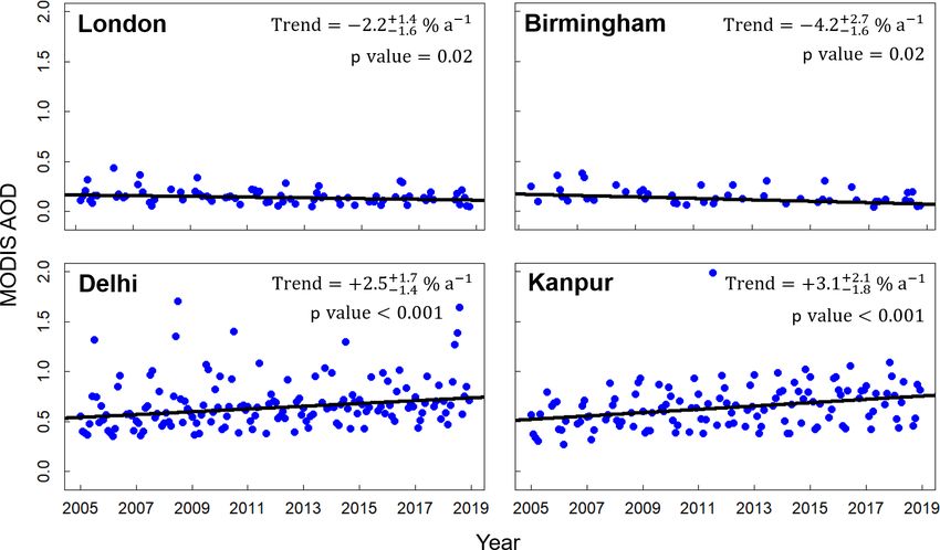
6286                                                             K. Vohra et al.: Long-term trends in air quality in major cities

Figure 8. Time series of IASI NH3 in 2008–2018 for London, Birmingham, Delhi, and Kanpur. Points are city-average monthly means. Black
lines are trends obtained with the Theil–Sen single median estimator. The grey lines are the fit (solid) and trend component (B) (dashed)
obtained with Eq. (1). Values inset are annual trends and p values for the Theil–Sen fit (in black) and annual trends obtained with Eq. (1)
(grey). Trend errors (not shown) exceed ±150 % in all cities.

atures enhancing emissions of isoprene, a dominant HCHO                    According to the UK bottom-up emission inventory, na-
precursor in India (Surl et al., 2018; Chalilyakunnel et al.,           tional NMVOCs emissions decreased by 2.4 % a−1 from
2019). The trends suggest reactive NMVOCs emissions have                2005 to 2017 (Defra, 2019a). This is supported by decline
decreased in Birmingham (1.6 % a−1 ) and increased in Lon-              in short-chain hydrocarbons measured at Harwell from 2–
don (0.5 % a−1 ), Delhi (1.9 % a−1 ), and Kanpur (1.0 % a−1 ).          3 µg m−3 in 2008 to 0.8–0.9 µg m−3 in 2015. These include
Only Delhi has a significant trend. The spread in values in-            hydrocarbons from vegetation (isoprene and monoterpenes)
creases for Delhi and Kanpur from 19 %–24 % relative to the             and vehicles (light alkanes and aromatics) but exclude oxy-
trend line in 2005 to 31 %–40 % in 2018. The change in the              genated VOCs (OVOCs) that in the UK include increas-
spread of values does not appear to be due to loss of data re-          ing contributions from domestic combustion, the food and
sulting from the row anomaly, as the change in the spread of            beverage industry, and household products (Defra, 2019a).
HCHO over time is similar if we remove all pixels affected              OVOCs have relatively high HCHO yields (Millet et al.,
by the row anomaly for the entire data record (2005–2018).              2006), and VOC concentrations measured during field cam-
OMI HCHO slant columns (HCHO along the instrument                       paigns in London and cities in India, including Delhi, are
viewing path) remain relatively stable throughout the OMI               dominated by OVOCs (> 60 % in London) (Valach et al.,
record (Zara et al., 2018), so the increase in variability may          2014; Sahu et al., 2016; L. Wang et al., 2020). In London,
reflect more extreme emissions from seasonal sources like               OVOCs also dominate inferred fluxes of VOCs (Langford
open fires in the IGP (Jethva et al., 2019). The trends from            et al., 2010) and reactivity of VOCs with the main atmo-
satellite observations of HCHO in megacities obtained by De             spheric oxidant, OH (Whalley et al., 2016). The rapid in-
Smedt et al. (2010) using multiple instruments for 1997–                crease in HCHO also has implications for ozone air pollu-
2009 are consistent with ours for Delhi (1.6 ± 0.7 % a−1 )              tion and the radical budget in London, as ozone formation
but opposite for London (−0.4 ± 2.1 % a−1 ). There is a shift           is VOC-limited, and HCHO photolysis is the second largest
in the magnitude of the HCHO trend for London around                    source of hydrogen oxide radicals (HOx ≡ OH + HO2 ) in
2011 (Fig. 9) from an increase of 0.3 % a−1 (p value = 0.9)             London (Whalley et al., 2018).
in 2005–2011 to a rapid increase of 9.3 % a−1 (95 % CI:                    Figure 10 shows the time series of city-average MODIS
0 % a−1 –26 % a−1 ) in 2012–2018. Visually the data suggest             AOD monthly means in the four cities for 2005–2018. Trends
a decline in OMI HCHO in 2005–2011, as in De Smedt et                   in AOD are significant in all four cities and range from a de-
al. (2010), but our trend estimate for 2005–2011 is affected            cline of 4.2 % a−1 in Birmingham to an increase of 3.1 % a−1
by a limited analysis period and large interannual variability.         in Kanpur. Mean AOD in Delhi and Kanpur is on average 5–

Atmos. Chem. Phys., 21, 6275–6296, 2021                                                    https://doi.org/10.5194/acp-21-6275-2021
K. Vohra et al.: Long-term trends in air quality in major cities 6287
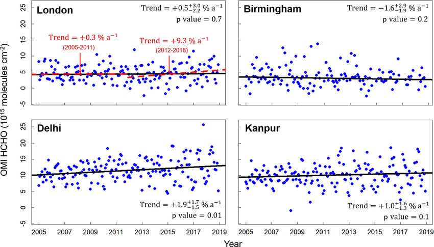
Figure 9. Time series of OMI HCHO for London, Birmingham, Delhi, and Kanpur. Points are city-average monthly means of OMI HCHO
after removing the background contribution (see text for details). Solid black lines are trends for 2005–2018 obtained with the Theil–Sen
single median estimator. Values inset are annual trends and p values. Absolute errors on the trends are the 95 % CI. Dashed red lines show
trend lines for London in 2005–2011 and 2012–2018, and red text shows corresponding annual trends.
6 times more than in London and Birmingham, due to large four cities: two in the UK (London and Birmingham) and
local anthropogenic emissions, nearby agricultural emissions two in India (Delhi and Kanpur).
of PM2.5 and its precursors in the IGP, and long-range trans- Assessment of satellite observations against ground-based
port of desert dust (David et al., 2018). Our results, as abso- measurements followed careful screening of the in situ mea-
lute AOD trends for London (−0.004 a−1 ) and Birmingham surements for poor-quality data, correcting NO2 data re-
(−0.007 a−1 ) for 2005–2018, are similar to trends obtained ported in inconsistent units at monitoring sites in Delhi and
by Pope et al. (2018) for 2005–2015 (−0.006 a−1 for Lon- Kanpur and removing sites influenced by local sources. OMI
don; −0.005 a−1 for Birmingham). Our trends for both cities NO2 reproduces monthly variability in surface concentra-
in India are less steep than the increase for Delhi (4.9 % a−1 ) tions of NO2 in cities, whereas satellite AOD reproduces
obtained for 2000–2010 with the MODIS 10 km AOD prod- trends, but not monthly variability, in PM2.5 in cities. MODIS
uct (Ramachandran et al., 2012) and for Kanpur (10.3 % a−1 ) and AERONET AOD are consistent at long-term monitor-
obtained for 2001–2010 with AERONET AOD at the Kanpur ing sites in Kanpur and a UK EMEP site in southern Eng-
AERONET site (Kaskaoutis et al., 2012). This may reflect a land. IASI NH3 is consistent with monthly variability in sur-
recent dampening of the trend or differences in data products face NH3 concentrations at two of three rural UK EMEP
and sampling domain/period. Sulfate from coal-fired power sites. There were no appropriate measurements of reactive
plants in India makes a large contribution to PM2.5 (Weagle NMVOCs to compare to OMI HCHO.
et al., 2018), and emissions from these nearly doubled from According to the long-term record from Earth observa-
2004 to 2015 (Fioletov et al., 2016). tions, NO2 , PM2.5 , and NMVOCs increased in Delhi and
Kanpur. There is no reversal in the increase in NO2 or PM2.5
in Delhi or Kanpur, as would be expected from successful
5 Conclusions implementation of air pollution mitigation measures. In all
four cities, the magnitude and direction of trends in NH3
Satellite observations of atmospheric composition provide are sensitive to treatment of NH3 seasonality, and none of
long-term and consistent global coverage of air pollutants. the NH3 trends are significant. In London and Birmingham,
We assessed the ability of satellite observations of nitrogen NO2 and PM2.5 decrease, and HCHO, a proxy for reactive
dioxide (NO2 ) and formaldehyde (HCHO) from OMI for NMVOCs emissions, decreases in Birmingham but exhibits
2005–2018, ammonia (NH3 ) from IASI for 2008–2018, and a recent (2012–2018) sharp (> 9 % a−1 ) increase in London.
aerosol optical depth (AOD) from MODIS for 2005–2018 This may reflect increased emissions of oxygenated VOCs
to provide constraints on long-term changes in city-average and long-chain hydrocarbons from household products, the
NO2 , reactive NMVOCs, NH3 , and PM2.5 , respectively in food and beverage industry, and residential fuelwood burn-
https://doi.org/10.5194/acp-21-6275-2021 Atmos. Chem. Phys., 21, 6275–6296, 2021You can also read