Retrieving the global distribution of the threshold of wind erosion from satellite data and implementing it into the Geophysical Fluid Dynamics ...
←
→
Page content transcription
If your browser does not render page correctly, please read the page content below
Atmos. Chem. Phys., 20, 55–81, 2020
https://doi.org/10.5194/acp-20-55-2020
© Author(s) 2020. This work is distributed under
the Creative Commons Attribution 4.0 License.

Retrieving the global distribution of the threshold of wind erosion
from satellite data and implementing it into the Geophysical Fluid
Dynamics Laboratory land–atmosphere model (GFDL
AM4.0/LM4.0)
Bing Pu1,2,a , Paul Ginoux2 , Huan Guo2 , N. Christina Hsu3 , John Kimball4 , Beatrice Marticorena5 , Sergey Malyshev2 ,
Vaishali Naik2 , Norman T. O’Neill6 , Carlos Pérez García-Pando7,8 , Juliette Paireau9,10 , Joseph M. Prospero11 ,
Elena Shevliakova2 , and Ming Zhao2
1 Atmospheric    and Oceanic Sciences Program, Princeton University, Princeton, New Jersey 08544, USA
2 NOAA    Geophysical Fluid Dynamics Laboratory, Princeton, New Jersey 08540, USA
3 NASA Goddard Space Flight Center, Greenbelt, Maryland 20771, USA
4 Department of Ecosystem and Conservation Sciences, University of Montana, Missoula, Montana 59812, USA
5 Laboratoire Interuniversitaire des Systèmes Atmosphériques, Universités Paris Est-Paris Diderot-Paris 7,

UMR CNRS 7583, Créteil, France
6 Département de géomatique appliquée, Université de Sherbrooke, Sherbrooke, Canada
7 Barcelona Supercomputing Center, 08034 Barcelona, Spain
8 ICREA, Passeig Lluís Companys 23, 08010 Barcelona, Spain
9 Department of Ecology and Evolutionary Biology, Princeton Environmental Institute, Princeton University,

Princeton, New Jersey 08544, USA
10 Mathematical Modelling of Infectious Diseases Unit, Institut Pasteur, UMR 2000, CNRS, 75015 Paris, France
11 Rosenstiel School of Marine and Atmospheric Sciences, University of Miami, Miami, Florida 33149, USA
a current affiliation: Department of Geography & Atmospheric Science, the University of Kansas, Lawrence,

Kansas 66045, USA

Correspondence: Bing Pu (bing.pu@noaa.gov)

Received: 8 March 2019 – Discussion started: 19 March 2019
Revised: 28 October 2019 – Accepted: 21 November 2019 – Published: 3 January 2020

Abstract. Dust emission is initiated when surface wind ve-        PM10 dust concentrations, and the seasonal cycle of DOD
locities exceed the threshold of wind erosion. Many dust          are better captured over the “dust belt” (i.e., northern Africa
models used constant threshold values globally. Here we use       and the Middle East) by simulations with the new wind ero-
satellite products to characterize the frequency of dust events   sion threshold than those using the default globally constant
and land surface properties. By matching this frequency de-       threshold. The most significant improvement is the frequency
rived from Moderate Resolution Imaging Spectroradiometer          distribution of dust events, which is generally ignored in
(MODIS) Deep Blue aerosol products with surface winds,            model evaluation. By using monthly rather than annual mean
we are able to retrieve a climatological monthly global distri-   Vthreshold , all comparisons with observations are further im-
bution of the wind erosion threshold (Vthreshold ) over dry and   proved. The monthly global threshold of wind erosion can
sparsely vegetated surfaces. This monthly two-dimensional         be retrieved under different spatial resolutions to match the
threshold velocity is then implemented into the Geophysical       resolution of dust models and thus can help improve the sim-
Fluid Dynamics Laboratory coupled land–atmosphere model           ulations of dust climatology and seasonal cycles as well as
(AM4.0/LM4.0). It is found that the climatology of dust op-       dust forecasting.
tical depth (DOD) and total aerosol optical depth, surface

Published by Copernicus Publications on behalf of the European Geosciences Union.
56                                            B. Pu et al.: Retrieving the global distribution of the threshold of wind erosion

1    Introduction                                                    Hamburg version of the European Centre for Medium-Range
                                                                     Weather Forecasts (ECMWF) model Hamburg Aerosol Mod-
Mineral dust is one of the most abundant aerosols by mass            ule (ECHAM-HAM), Hadley Centre Global Environmental
and plays an important role in the climate system. Dust par-         Model, version 2, Earth System (HadGEM2-ES), and ICOsa-
ticles absorb and scatter solar and terrestrial radiation, thus      hedral Nonhydrostatic – Aerosol and Reactive Trace gases
modifying the local energy budget and consequently atmo-             (ICON-ART), parameterize the constant dry threshold fric-
spheric circulation patterns. Studies have shown that the ra-        tion velocity (usually a function of soil particle size, soil, and
diative effect of dust can affect a wide range of environmental      air density) or threshold wind velocity with dependencies on
processes. Dust is shown to modulate western African (e.g.,          soil moisture, surface roughness length, and vegetation cov-
Miller and Tegen, 1998; Miller et al., 2004; Mahowald et al.,        erage (e.g., Takemura et al., 2000; Ginoux et al., 2001; Zen-
2010; Strong et al., 2015) and Indian (e.g., Jin et al., 2014,       der et al., 2003; Cheng et al., 2008; Jones et al., 2011; Rieger
2015, 2016; Vinoj et al., 2014; Solmon et al., 2015; Kim             et al., 2017).
et al., 2016; Sharma and Miller, 2017) monsoonal precipi-               The threshold of wind erosion may be approximately
tation. During severe droughts in North America, there is a          inferred using observations. For instance, Chomette et
positive feedback between dust and the hydrological cycle            al. (1999) used the Infrared Difference Dust Index (IDDI)
(Cook et al., 2008, 2009, 2013). African dust is also found          and 10 m winds reanalysis from the ECMWF between 1990
to affect Atlantic tropical cyclone activity (e.g., Dunion and       and 1992 to calculate the threshold of wind erosion over
Velden, 2004; Wong and Dessler, 2005; Evan et al., 2006;             seven sites over the Sahel and Sahara. The IDDI was used
Strong et al., 2018). When deposited on snow and ice, dust           to determine whether there was a dust event for subsequently
reduces the surface reflectivity, enhancing net radiation and        calculating an emission index defined as the number of dust
accelerating snow and ice melting and consequently affect-           events to the total number of potential events. The distribu-
ing runoff (e.g., Painter et al., 2010, 2018; Dumont et al.,         tion of surface wind speed was matched with the emission in-
2014). Dust can serve as ice nuclei and affect the formation,        dex, and the threshold of wind erosion was determined when
lifetime, and characteristic of clouds (e.g., Levin et al., 1996;    the emission index was around 0.9. The resulting average
Rosenfield et al., 1997; Wurzler et al., 2000; Nakajima et al.,      threshold of wind erosion ranged from 6.63 m s−1 at a Sa-
2001; Bangert et al., 2012), perturbing the hydrological cy-         helian site to about 9.08 m s−1 at a Niger site, consistent with
cle. Iron- and phosphorus-enriched dust is also an important         the model results by Marticorena et al. (1997).
nutrient for the marine and terrestrial ecosystems and thus in-         Later, Kurosaki and Mikami (2007) used World Meteoro-
teracts with the ocean and land biogeochemical cycles (e.g.,         logical Organization (WMO) station data from March 1998
Fung et al., 2000; Jickells et al., 2005; Shao et al., 2011; Bris-   to June 2005 to examine the threshold wind speed in eastern
tow et al., 2010; Yu et al., 2015).                                  Asia. Using the distribution of surface wind speed and as-
   Given the importance of mineral dust, many climate mod-           sociated weather conditions (i.e., with or without dust emis-
els incorporate dust emission schemes to simulate the life           sion events), they approximated a dust emission frequency
cycle of dust aerosols (e.g., Donner et al., 2011; Collins et        by dividing the number of dust events by the total number
al., 2011; Watanabe et al., 2011; Bentsen et al., 2013). Min-        of observations for each wind bin, and then they determined
eral dust particles are lifted from dry and bare soils into          threshold wind speeds at the 5 % and 50 % levels, corre-
the atmosphere by saltation and sandblasting. This process           sponding to the most favorable and normal land surface con-
is initiated when surface winds reach a threshold velocity           ditions for dust emission, respectively. They found that the
of wind erosion. The value of this wind erosion threshold            derived threshold wind speed varied in space and time, with
depends on soil and surface characteristics, including soil          a larger seasonal cycle in grassland regions, such as north-
moisture, soil texture, and particle size, and the presence of       ern Mongolia, and smaller seasonal variations in desert re-
pebbles, rocks, and vegetation residue (e.g., Gillette et al.,       gions, such as the Taklimakan and Gobi deserts and the Loess
1980; Gillette and Passi, 1988; Raupach et al., 1993; Fécan          Plateau. Cowie et al. (2014) applied a similar method over
et al., 1999; Zender et al., 2003; Mahowald et al., 2005),           northern Africa, using wind data observed between 1984 and
and this thus varies spatially and temporally (Helgren and           2012, and they focused on threshold winds at the 25 %, 50 %,
Prospero, 1987). Due to a lack of in situ data at a global           and 75 % levels.
scale and uncertainties on these dependencies, most dust                Draxler et al. (2010) derived the distribution of the thresh-
and climate models prescribe a spatially and temporally con-         old of friction velocity over the US by matching the fre-
stant threshold of wind erosion for surface 10 m wind (e.g.,         quency of occurrence (FoO) of Moderate Resolution Imaging
around 6 to 6.5 m s−1 ) over dry surfaces for simplicity (e.g.,      Spectroradiometer (MODIS) Deep Blue (Hsu et al., 2004)
Tegen and Fung, 1994; Takemura et al., 2000; Uno et al.,             aerosol optical depth (AOD) above 0.75 with the FoO of fric-
2001; Donner et al., 2011). For instance, in the Geophysical         tion velocities extracted from the North American Mesoscale
Fluid Dynamics Laboratory coupled land–atmosphere model              (NAM) forecast model at each grid point. This new thresh-
AM4.0/LM4.0 (Zhao et al., 2018a, b), a constant threshold of         old and a soil characteristics factor was then incorporated
6 m s−1 is used. On the other hand, some models, such as the         into the Hybrid Single-Particle Lagrangian Integrated Trajec-

Atmos. Chem. Phys., 20, 55–81, 2020                                                      www.atmos-chem-phys.net/20/55/2020/
B. Pu et al.: Retrieving the global distribution of the threshold of wind erosion                                                57

tory (HYSPLIT) model (Draxier and Hess, 1998) to forecast              nent (α). All the daily variables are first interpolated to a
dust surface concentrations. It was found that major observed          0.1 × 0.1◦ grid using the algorithm described by Ginoux
dust plume events in June and July 2007 were successfully              et al. (2010). We require the single-scattering albedo at
captured by the model. Later, Ginoux and Deroubaix (2017)              470 nm to be less than 0.99 for dust due to its absorption
used FoO derived from the MODIS Deep Blue dust optical                 of solar radiation. This separates dust from scattering
depth (DOD) record to retrieve the wind erosion threshold of           aerosols, such as sea salt. Then a continuous function
surface 10 m winds over eastern Asia.                                  relating the Ångström exponent, which is highly sensi-
   For individual dust events, the threshold of friction veloc-        tive to particle size (Eck et al., 1999), to fine-mode AOD
ity can also be determined by fitting a 2nd-order Taylor series        established by Anderson et al. (2005; their Eq. 5) is used
to dust saltation flux measurements (Barchyn and Hugen-                to separate dust from fine particles. In short, DOD is re-
holtz, 2011; Kok et al., 2014b).                                       trieved using the following equation:
   Nonetheless, a global distribution of the threshold of wind
erosion with observational constraints that may be imple-              DOD = AOD × (0.98 − 0.5089α + 0.0512α 2 ).               (1)
mented in climate models is still lacking. In this study, we
propose a method to retrieve the monthly global threshold              Details about the retrieval process and estimated er-
of wind erosion (hereafter, Vthreshold ) for dry and sparsely          rors are summarized by Pu and Ginoux (2018b). High-
vegetated surface (i.e., under favorable conditions for dust           resolution MODIS DOD products (0.1 × 0.1◦ ) have
emission) using high-resolution satellite products and re-             been used to identify and characterize dust sources (Gi-
analysis datasets. This two-dimensional threshold of sur-              noux et al., 2012; Baddock et al., 2016) and examine the
face 10 m winds is then implemented into the Geophys-                  variations in dustiness in different regions (e.g., Pu and
ical Fluid Dynamics Laboratory (GFDL) coupled land–                    Ginoux, 2016, 2017, 2018b).
atmosphere model, AM4.0/LM4.0 (Zhao et al., 2018a, b).                 Following the recommendation from Baddock et
The benefits of using this spatially and temporally varying            al. (2016), who found the dust sources are better de-
threshold in simulating present-day climatology and seasonal           tected using DOD with a low-quality flag (i.e., qual-
cycles of dust are analyzed by comparing the model results             ity assurance flag, QA, equals 1, following the cate-
with observations.                                                     gory of retrieval quality flags in MODIS Deep Blue
   The data and method used to retrieve the threshold of wind          products; Hsu et al., 2013) than with a high-quality
erosion are detailed in Sect. 2. The distribution of the derived       flag (i.e., QA = 3); as retrieved aerosol products were
Vthreshold and its implication in the climate model is presented       poorly flagged over dust source regions, we also use
in Sect. 3. Section 4 discusses the uncertainties associated           DOD with the flag of QA = 1. Both daily DOD retrieved
with this method, and major conclusions are summarized in              from Aqua and Terra platforms are used by averaging
Sect. 5.                                                               the two when both products are available or using ei-
                                                                       ther one when only one product is available. Since Terra
                                                                       passes the Equator from north to south around 10:30 lo-
2     Data and methodology
                                                                       cal time (LT) and Aqua passes the Equator from south to
In this section we first introduce the satellite products, obser-      north around 13:30 LT, an average of the two combines
vational data, and reanalyses used to retrieve the threshold of        the information from both morning and afternoon hours.
wind erosion and validate model output (Sect. 2.1). The pro-           This process also largely reduces missing data (Pu and
cesses to retrieve the threshold of wind erosion are detailed          Ginoux, 2018b). This combined daily DOD, hereafter
in Sect. 2.2. The uncertainties of Vthreshold associated with          MODIS DOD, is available from January 2003 to De-
the retrieval criteria and selection of surface wind datasets          cember 2015 at a resolution of 0.1 × 0.1◦ grid. Note
are discussed in Sect. 2.3. Section 2.4 introduces the GFDL            that due to the temporal coverage of MODIS products,
AM4.0/LM4.0 model, its dust emission scheme, and simula-               the diurnal variations in dust (e.g., O’rgill and Sehmel,
tion designs.                                                          1976; Mbourou et al., 1997; Knippertz, 2008; Schepan-
                                                                       ski et al., 2009) are not included in current study.
2.1     Data
                                                                    2. Soil moisture. Soil moisture is an important factor that
2.1.1    Satellite products                                            affects dust emission (Fécan et al., 1999). Daily sur-
                                                                       face volumetric soil moisture (VSM) retrievals derived
    1. MODIS Aqua and Terra dust optical depth. DOD                    from similar calibrated microwave (10.7 GHz) bright-
       is column-integrated extinction by mineral particles.           ness temperature observations from the Advanced Mi-
       Here daily DOD is retrieved from MODIS Deep Blue                crowave Scanning Radiometer for the Earth Observing
       aerosol products (collection 6, level 2; Hsu et al.,            System (AMSR-E) onboard the NASA Aqua satellite
       2013; Sayer et al., 2013): aerosol optical depth (AOD),         (from June 2002 to October 2011) and the Advanced
       single-scattering albedo (ω), and the Ångström expo-            Microwave Scanning Radiometer 2 (AMSR2) sensor

www.atmos-chem-phys.net/20/55/2020/                                                      Atmos. Chem. Phys., 20, 55–81, 2020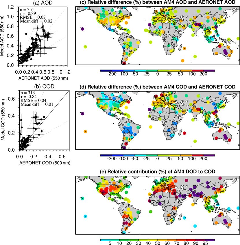
58                                          B. Pu et al.: Retrieving the global distribution of the threshold of wind erosion

     onboard the JAXA GCOM-W1 satellite (from July 2012          2.1.2     Reanalysis
     to June 2017) from the University of Montana (Du et al.,
     2017a, b) was used to retrieve the wind erosion thresh-     Surface wind speed is a critical factor that affects wind ero-
     old. Both AMSR-E and AMSR2 sensors provide global           sion. Here 6-hourly 10 m wind speed from the NCEP/NCAR
     measurements of polarized microwave emissions at six        (National Centers for Environmental Prediction/National
     channels, with ascending and descending orbits cross-       Center for Atmospheric Research) reanalysis (Kalnay et al.,
     ing the Equator at around 13:30 and 01:30 LT respec-        1996, hereafter NCEP1) on a T62 Gaussian grid (i.e., 192
     tively. The VSM retrievals are derived from an itera-       longitude grids equally spaced and 94 latitude grids un-
     tive retrieval algorithm that exploits the variable sen-    equally spaced) is used. The NCEP1 is a global reanalysis
     sitivity of different microwave frequencies and polar-      with relatively long temporal coverage, from 1948 to the
     izations and minimizes the potential influence of at-       present. We chose to use the NCEP1 reanalysis mainly be-
     mosphere, vegetation, and surface water cover on the        cause surface winds in the GFDL AM4.0 model are nudged
     soil signal. The VSM record represents surface (top         toward the NCEP1, and we preferred to use the reanalysis
     ∼ 2 cm) soil conditions and shows favorable global ac-      surface wind that is closest to the model climatology.
     curacy and consistent performance (Du et al., 2017b),          ERA-Interim (ECMWF Reanalysis Interim; Dee et al.,
     particularly over areas with low-to-moderate vegetation     2011) is a global reanalysis produced from ECMWF. It pro-
     cover that are also more susceptible to wind erosion, al-   vides high spatial resolution (about 0.75◦ or 80 km) 6-hourly,
     though cautions are needed when examining long-term         daily, and monthly reanalysis from 1979 to present day. Soil
     trends due to the small biases between AMSR-E and           temperature from the ERA-Interim is used to determine the
     AMSR2. The horizontal resolution of the product is          regions where wind erosion may be prohibited by the frozen
     about 25 km × 25 km, and the daily product from Jan-        surface. Monthly temperature of the first soil layer (0 to
     uary 2003 to December 2015 is used. The ascending and       0.07 m) from 2003 to 2015 is used.
     descending obit VSM retrievals are averaged to get the         In order to quantify the uncertainties of the retrieved
     mean VSM for each day.                                      threshold wind erosion in association with the selection of
                                                                 reanalysis products, surface 10 m winds from 6-hourly ERA-
 3. Snow cover. Snow cover may affect dust emission in           Interim and hourly ERA5 (Hersbach and Dee, 2016) are both
    the mid-latitudes during spring, for instance, over north-   examined. The ERA5 is the latest reanalysis product from the
    ern China (Ginoux and Deroubaix, 2017). The inter-           ECMWF, with a horizontal resolution of about 31 km and
    annual variation of snow cover is also found to affect       hourly temporal resolution.
    dust emission in regions such as Mongolia (Kurosaki
    and Mikami, 2004). Here monthly snow cover data from         2.1.3     Station data
    MODIS/Terra level 3 data (Hall and Riggs, 2015) with a
    resolution of 0.05 × 0.05◦ from 2003 to 2015 are used.       Multiple ground-based datasets are used to validate
    The high spatial resolution of the product is very suit-     AM4.0/LM4.0 simulated aerosol and dust optical depth and
    able for this study.                                         surface dust concentrations.
 4. Leaf area index (LAI). Vegetation protects soil from the       1. AERONET. The AErosol RObotic NETwork
    effects of wind and thus modulates dust emission (e.g.,           (AERONET; Holben et al., 1998) provides quality-
    Marticorena and Bergametti, 1995; Zender et al., 2003).           assured cloud-screened (level 2) aerosol measurements
    While dense vegetation coverage can increase surface              from sun photometer records. In this paper we used the
    roughness and reduce near-surface wind speed, the roots           data products of the version 3.0 AERONET processing
    of vegetation can increase soil cohesion and further re-          routine. To examine model-simulated DOD, we used
    duce wind erosion. LAI describes the coverage of veg-             coarse-mode AOD (COD; i.e., radius > 0.6 µm) at
    etation with a unit of m2 m−2 , i.e., leaf area per ground        500 nm processed by the Spectral Deconvolution
    area. Here monthly LAI retrieved by Boston University             Algorithm (O’Neill et al., 2003; hereafter SDA). SDA
    from MODIS onboard Aqua (Yan et al., 2016a, b; Ranga              COD monthly data are first screened to remove those
    Myneni and Taejin Park, Boston University, personal               months with less than 5 d of records. To get the annual
    communication, 2016) with a resolution of 0.1 × 0.1◦              means, years with less than 5 months of records were
    from 2003 to 2015 is used. The root mean square error             removed. Only stations with records of at least 3 years
    of the product is 0.66, with some overestimation of LAI           during the period were used to calculate the 2003–2015
    in sparsely vegetated regions (Yan et al. 2016b; Gar-             climatology (the same time period when MODIS DOD
    rigues et al., 2008).                                             is available). Overall, records from 313 stations were
                                                                      obtained.
                                                                         AERONET monthly aerosol optical thickness (AOT)
                                                                         data around 550 nm (e.g., 500, 551, 531, 440, 675,

Atmos. Chem. Phys., 20, 55–81, 2020                                                     www.atmos-chem-phys.net/20/55/2020/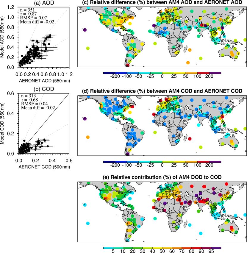
B. Pu et al.: Retrieving the global distribution of the threshold of wind erosion                                           59

    490, 870 nm, etc.) and the Ångström exponents across            station records end earlier than 1998, the dataset largely
    the dual wavelength of 440–675, 440–870, and 500–               represents the climatology during the 1980s and 1990s.
    870 nm are used to calculate AOD at 550 nm (τ550 ).             Thus the discrepancies between model output and the
    If AOT for 551, 555, 531 or 532 nm exist, then these            RSMAS data include both model biases and the differ-
    values are directly used as AOD 550 nm. Otherwise,              ence in surface dust concentration from the 1980s to the
    the AOT at wavelength λA (less than 550 nm; i.e., τA ),         2000s.
    AOT at wavelength λB (larger than 550 nm; i.e., τB ),
    and Ångström exponent between wavelengths λA and             3. IMPROVE surface fine dust concentration. The Inter-
    λB (α) are used to derive AOD 550 nm using the fol-             agency Monitoring of Protected Visual Environments
    lowing equations:                                               (IMPROVE) network has collected near-surface partic-
                                                                    ulate matter 2.5 (PM2.5 ) samples in the US since 1988

                    550
                          −α                                       (Malm et al., 1994; Hand et al., 2011). IMPROVE sta-
    τ550 = τA                   if τA i s available,      (2)       tions are located in national parks and wilderness ar-
                    λA
                         −α                                       eas, and PM2.5 sampling is performed twice weekly
                    550                                             (Wednesday and Saturday; Malm et al., 1994) prior to
    τ550 = τB                   if τB is available.       (3)
                    λB                                              2000 and every third day afterwards. Fine dust (with an
                                                                    aerodynamic diameter less than 2.5 µm) concentration is
    In a manner similar to the process of screening SDA             calculated using the concentrations of aluminum (Al),
    COD data, monthly AOD 550 nm data with less than 3 d            silicon (Si), calcium (Ca), iron (Fe), and titanium (Ti)
    of records in a given month are removed. When calcu-            by assuming oxide norms associated with predominant
    lating the annual means we excluded years having less           soil species (Malm et al., 1994; their Eq. 5). This dataset
    than 5 months of records. Finally, to calculate the clima-      has been widely used to study variations in surface fine
    tology of 2003–2015, only stations with at least 3 years        dust in the US (e.g., Hand et al., 2016, 2017, Tong et al.,
    of records during this period are used, totaling 351.           2017; Pu and Ginoux, 2018a). Here only monthly data
    We also developed a method to derive DOD at 550 nm              with at least 50 % of the daily data available in a month
    from AOD at 550 nm based on the relationship between            (i.e., at least 5 records) are used. Since station cover-
    the Ångström exponent and fine-mode AOD established             age over the central US increases after 2002 (e.g., Pu
    by Anderson et al. (2005; their Eq. 5). This adds a few         and Ginoux, 2018a), monthly station data from 2002 to
    more sites over the Sahel than the SDA COD stations.            2015 are used and interpolated to a 0.5 × 0.5◦ grid us-
    DOD is calculated by subtracting fine-mode AOD from             ing inverse distance weighting interpolation. The grid-
    total AOD. Due to the large uncertainties of single-            ded data are used to evaluate modeled surface fine dust
    scattering albedo in AERONET records over regions               concentrations.
    where AOD is lower than 0.4 (e.g., Dubovik and King,         4. LISA PM10 surface concentration. Surface PM10 con-
    2000; Holben et al., 2006; Andrews et al., 2017), we did        centrations from stations from the Sahelian Dust Tran-
    not use single-scattering albedo to screen AOD to fur-          sect, which was deployed in 2006 under the framework
    ther separate dust from scattering aerosols. Therefore,         of the African Monsoon Multidisciplinary Analysis In-
    the derived AERONET DOD over coastal stations may               ternational Program (Marticorena et al., 2010), were
    be contaminated by sea salt.                                    used to examine the surface dust concentration over the
 2. RSMAS surface dust concentration. The Rosenstiel                Sahelian region. The data are maintained by the Labo-
    School of Marine and Atmospheric Science (hereafter             ratoire Interuniversitaire des Systèmes Atmosphériques
    the RSMAS dataset) at the University of Miami col-              (LISA) in the framework of the International Network
    lected mass concentrations of dust, sea salt, and sulfate       to study Deposition and Atmospheric composition in
    over stations globally, with most of the stations on is-        Africa (INDAAF; Service National d’Observation de
    lands (Savoie and Prospero, 1989). The dataset has been         l’Institut National des Sciences de l’Univers, France).
    widely used for model evaluation (e.g., Ginoux et al.,          Three stations are located within the pathway of Saha-
    2001; Huneeus et al., 2011).                                    ran and Sahelian dust plumes moving towards the At-
                                                                    lantic Ocean. Here hourly PM10 concentrations from
    Only stations with records longer than 4 years were             the stations in Banizoumbou (Niger, 13.54◦ N, 2.66◦ E),
    used, and of those stations only those years with at least      Cinzana (Mali, 13.28◦ N, 5.93◦ W), and M’Bour (Sene-
    8 months of data are used for calculating climatologi-          gal, 14.39◦ N, 16.96◦ W) from 2006 to 2014 are used.
    cal annual means. So, in total 16 stations are used. Sta-       The hourly station data are averaged to obtain daily and
    tion names, locations, and record lengths are listed in         monthly mean records to compare with model output.
    Table S1 of the Supplement. We compare the clima-
    tology of annual mean surface dust concentration with
    model output during 2000–2015. Note that since most

www.atmos-chem-phys.net/20/55/2020/                                                  Atmos. Chem. Phys., 20, 55–81, 2020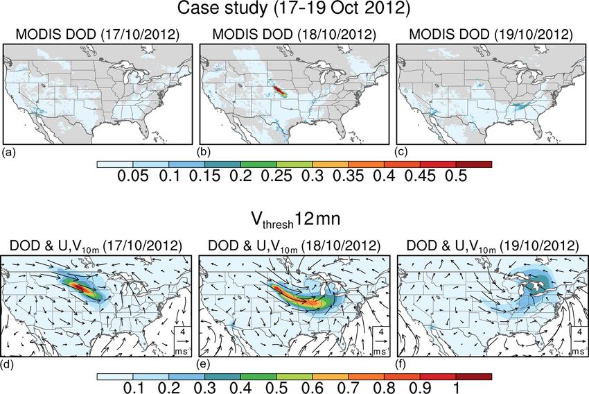
60 B. Pu et al.: Retrieving the global distribution of the threshold of wind erosion
2.1.4 Other data dust emission only occurs when wind speed is strong
enough, and the emission magnitude is roughly propor-
Soil depth from the Food and Agriculture Organization of the tional to the third power of surface wind speed in empir-
United Nations (FAO/IIASA/ISRIC/ISS-CAS/JRC, 2009) on ical estimations. The cumulative frequency distribution
a 0.08 × 0.08◦ resolution is used to examine whether the soil of daily maximum surface wind from 2003 to 2015 is
depth is too shallow (i.e., less than 15 cm) for wind erosion. then calculated at each grid point for each month.
2.2 Retrieving the threshold of wind erosion – Step 4. A minimum value of DOD (i.e., DODthresh ) is
used to separate dust events from background dust. The
The monthly climatological threshold of wind erosion is re-
cumulative frequency (as a percentage) of dust events
trieved by matching the frequency distribution of the MODIS
passing this threshold is compared to the cumulative fre-
DOD at a certain level, namely, DODthresh , with the fre-
quency of surface winds. The minimum surface winds
quency distribution of surface 10 m winds from the NCEP1
with the same frequency correspond to the threshold
reanalysis over the period from 2003 to 2015. The process
of wind erosion, Vthreshold (see a schematic diagram
can be summarized by the following steps:
in Fig. S1 in the Supplement). This operation is per-
– Step 1. Since dust is emitted from the dry and sparsely formed for all grid points for each month. Ginoux et
vegetated surface, the daily DOD data are first masked al. (2012) used DODthresh = 0.2 to separate dust events
out to remove the influences of non-erodible factors and from background dust and quantify the FoO of local
unfavorable environmental conditions that are known to dust events. Similarly, DODthresh = 0.2 is used here in
prevent dust emission using criteria as follows: daily major dusty regions (northern Africa, the Middle East,
VSM less than 0.1 cm3 cm−3 ; monthly LAI less than India, northern China), while for less dusty regions,
0.3; monthly snow cover less than 0.2 % (since the such as the US, South America, South Africa, and Aus-
snow cover percentage is rounded up to an integer in tralia, DODthresh = 0.02 is used. The reason to use a
the MODIS product, this criterion actually requires no lower DODthresh for less dusty regions is because (i) the
snow cover); monthly top-layer soil temperature higher overall dust emission in these regions are at least 10
than 273.15 K, i.e., over unfrozen surface; and soil depth times smaller than major dusty regions, such as north-
thicker than 15 cm. These criteria approximate the most ern Africa (e.g., Huneeus et al., 2011) and (ii) the fre-
favorable land surface conditions for wind erosion. quency distribution of DOD in these regions also peaks
at a much lower DOD band (see discussion in Sect. 3.3).
Similar criteria have been used in previous studies to
We also tested the DODthresh = 0.5 for dusty regions
detect or confine dust source regions. For instance, Kim
and DODthresh = 0.05 for less dusty regions, and results
et al. (2013) used the normalized difference vegeta-
are discussed in Sects. 2.3 and 3.1.
tion index (NDVI) for less than 0.15, soil depth greater
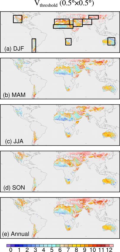
than 10 cm, surface temperature greater than 260 K, Figure 1a–e show the seasonal and annual mean FoO
and without snow cover to mask topography-based dust (days when DOD is greater than DODthresh ) using
source function. LAI less than 0.3 has been used as DODthresh = 0.2 or 0.02. The shaded area covers ma-
a threshold for dust emission in the Community Land jor dust sources, and the pattern is very similar to that
Model (Mahowald et al., 2010; Kok et al., 2014a), while obtained by Ginoux et al. (2012; their Fig. 5), although
gravimetric soil moisture ranging from 1.01 % to 11.2 % there are some differences, largely due to the masked
depending on soil clay content is recommended to con- DOD (i.e., from Step 1) used in this study and a lower
strain dust emission (Fécan et al., 1999). The uncertain- threshold in less dusty regions. The higher FoO in north-
ties associated with small variations in the retrieval cri- ern Africa during summer in comparison with other
teria are further quantified and discussed in Sect. 2.3. seasons is consistent with the summer peak of the fre-
quency of the dust source activation derived from the
– Step 2. Masked daily DOD from Step 1 is then inter- Meteosat Second Generation (MSG) images (Schepan-
polated to a 0.5 × 0.5◦ grid using bilinear interpolation. ski et al., 2007; their Fig. 1). The relatively high value of
This is close to the horizontal resolution of the GFDL FoO over the northern Sahel to southern Sahara is also
AM4.0/LM4.0 model used in this study. Then the cumu- consistent with dust emission frequency derived from
lative frequency distribution of daily DOD from 2003 to the Meteosat Second Generation Spinning Enhanced
2015 is derived at each grid point for each month. Visible and Infrared Imager (Evan et al., 2015; their
Fig. 1).
– Step 3. Daily maximum surface wind speed is first de-
rived from 6-hourly NCEP1 surface winds and then Note that the selections of masking criteria in Step 1 and
interpolated to a 0.5 × 0.5◦ grid. Following Ginoux DODthresh in Step 4 are empirical and can add uncertain-
and Deroubaix (2017), we use maximum daily wind ties to this method. Also, we approximate dust emission
speed instead of daily mean wind speed, largely because using the cumulative frequency of DOD, which may
Atmos. Chem. Phys., 20, 55–81, 2020 www.atmos-chem-phys.net/20/55/2020/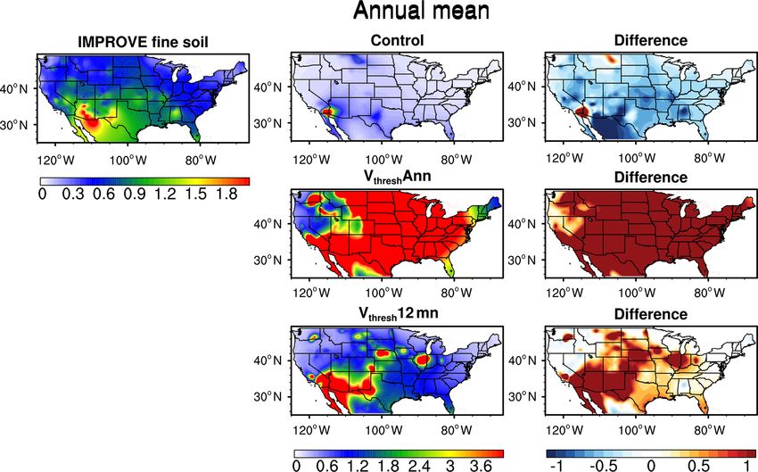
B. Pu et al.: Retrieving the global distribution of the threshold of wind erosion                                                           61

Figure 1. (a–e) Frequencies of occurrence (FoO; unit: days per season) in each season and the annual mean. (f–j) Threshold of wind erosion
(Vthreshold ; unit: m s−1 ) derived from satellite products and reanalyses for each season and the annual mean using DODthresh = 0.2 (or 0.02).
Black boxes in (f) denote nine dust source regions as listed in Table 1.

      overestimate dust emission in regions where the con-
      tribution of transported dust is significant, and thus we
      may underestimate the Vthreshold in those regions. These
                                                                          Table 1. Major dust source regions shown in Fig. 1. Note that region
      uncertainties are further discussed in the following sec-
                                                                          names such as India and northern China are not exactly the same
      tion.
                                                                          as their geographical definitions, as these regions also cover some
                                                                          areas from nearby countries.
2.3   Sensitivities of Vthreshold to retrieval criteria and the
      selection of reanalysis surface winds                                 No.    Regions                                      Coordinates
                                                                            1      Sahel                            10–20◦ N, 18◦ W–35◦ E
Table 2 shows variations in derived annual mean Vthreshold
                                                                            2      Sahara                           20–35◦ N, 15◦ W–25◦ E
averaged in nine dust source regions (see Table 1 for lo-                   3      Arabian Peninsula                    15–35◦ N, 35–60◦ E
cations) following slight changes of retrieval criteria: soil               4      Northern China (N. China)           35–45◦ N, 77–103◦ E
moisture, LAI, snow coverage, and DODthresh . When the soil                 5      India                                20–35◦ N, 60–85◦ E
moisture threshold is changed from 0.1 to 0.15 cm3 cm−3                     6      US                                25–45◦ N, 102–125◦ W
or without the soil moisture constraint, the variations in                  7      South Africa (S. Africa)              17–35◦ S, 15–30◦ E
Vthreshold are quite small, ranging from 0.01 to about 0.73                 8      South America (S. America)           18–55◦ S, 65–75◦ W
m s−1 (Table 2). Similarly, changes of LAI criteria from                    9      Australia                          15–35◦ S, 128–147◦ E
0.15 to 0.5 m2 m−2 or snow coverage from 0.2 % to 10 %
slightly change Vthreshold – within 1 m s−1 over most regions.
On the other hand, Vthreshold is quite sensitive to the se-

www.atmos-chem-phys.net/20/55/2020/                                                               Atmos. Chem. Phys., 20, 55–81, 2020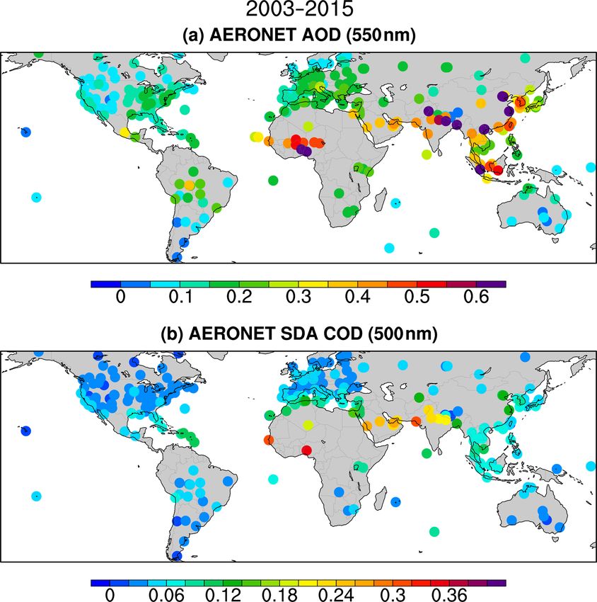
62                                                  B. Pu et al.: Retrieving the global distribution of the threshold of wind erosion

Table 2. Sensitivity of the annual mean wind erosion threshold (m s−1 ) to the selection of different retrieval criteria. Note the setting of the last
column is the same as DODthresh = 0.2 or 0.02, except surface DOD (sDOD) from Aqua is used over northern Africa. Here DODthresh = 0.2
or 0.5 is applied to dusty regions, i.e., the Sahel, Sahara, Arabian Peninsula, northern China, and India, while DODthresh = 0.02 or 0.05 is
applied to less dusty regions, i.e., the US, South Africa, South America, and Australia.

  Regions              Soil moisture (cm3 cm−3 )         LAI (m2 m−2 )                Snow coverage (%)                     DODthresh
                       < 0.1    < 0.15      None     < 0.15    < 0.3   < 0.5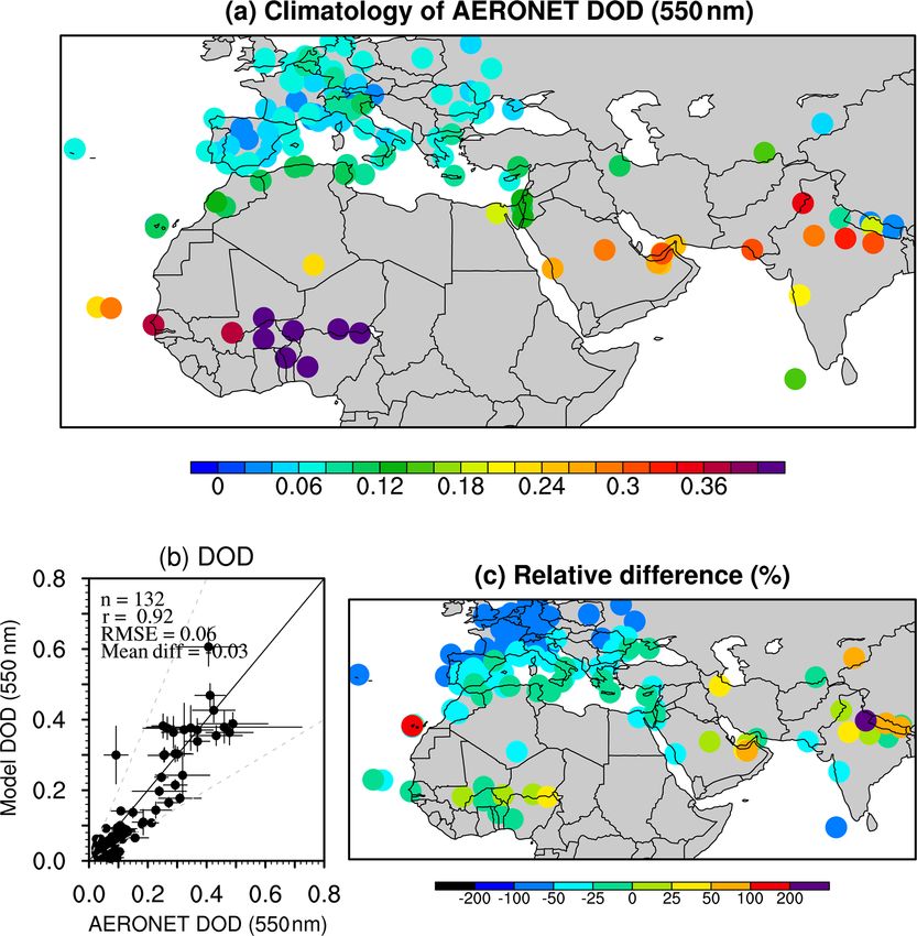
B. Pu et al.: Retrieving the global distribution of the threshold of wind erosion                                                  63

Table 4. Simulation design.                                          (Eq. 4) the same in all simulations to better examine the ef-
                                                                     fects of implementing the newly developed Vthreshold .
   Simulations     Wind erosion threshold    Source function            In the Control run, the default model setting is used for
                                                                     dust emission, with a prescribed 6 m s−1 threshold of wind
   Control         6 m s−1                          S
   Vthresh 12 mn   12-month Vthreshold              S0
                                                                     erosion (cf. Ginoux et al., 2019). In the Vthresh 12 mn simula-
   Vthresh Ann     Annual mean Vthreshold           S0               tion, the observation-based climatological monthly Vthreshold
                                                                     is used to replace the constant wind erosion threshold. The
                                                                     default source function S in Eq. (4) only allows dust emission
                                                                     over bare ground by masking out regions with vegetation
mulation, a double-plume model representing shallow and              cover. Since LAI masking is already applied in the retrieval
deep convection, a “light” chemistry mechanism, and modu-            of Vthreshold (i.e., LAI < 0.3), we choose to use a source func-
lation on aerosol wet removal by convection and frozen pre-          tion that is the same as the default source function S but
cipitation (Zhao et al., 2018a, b). Here we used a model ver-        without vegetation masking, i.e., S 0 (Fig. S2 in the Supple-
sion with 33 vertical levels (with a model top at 1 hPa) and         ment). This allows the influence of the spatial and temporal
cube sphere with 192×192 grid boxes per cube face (approx-           variations in Vthreshold to be fully examined. The combination
imately 50 km grid size).                                            of source function S 0 and Vthreshold also extends dust source
   The aerosol physics is based in large part on that of GFDL        from bare ground to sparsely vegetated areas as outlined by
AM3.0 (Donner et al., 2011), but it has a simplified chem-           Vthreshold , e.g., over central North America, central India, and
istry where ozone climatology from AM3.0 simulation (Naik            part of Australia, and that can increase dust emission in these
et al., 2013) is prescribed. AM4.0 simulates the mass distri-        regions. The pattern of extended dust source area largely re-
bution of five aerosols: sulfate, black carbon, organic carbon,      sembles the vegetated dust source identified by Ginoux et
dust, and sea salt. Dust is partitioned into five size bins based    al. (2012; their Fig. 15b) and Kim et al. (2013; their Fig. 9).
on radius: 0.1–1 µm (bin 1), 1–2 µm (bin 2), 2–3 µm (bin             All the other settings are the same as the Control run. The
3), 3–6 µm (bin 4), and 6–10 µm (bin 5). The dust emission           Vthresh Ann simulation is the same as the Vthresh 12 mn but uses
scheme follows the parameterization of Ginoux et al. (2001),         the annual mean Vthreshold for each month. Since the same
as shown in the following equation:                                  SST and sea ice are prescribed for all simulations and land
                                                                     use dose not change much during the short duration of sim-
                   2
Fp = C × S × sp × V10 m (V10 m − Vt ) (if V10 m > Vt ),        (4)   ulation, the differences in simulated dynamic vegetation by
                                                                     LM4.0 among the three simulations are actually very small
where Fp is the flux of dust of particle size class p, C is          and can be ignored (see Figs. S3–S4 in the Supplement).
a scaling factor with a unit of µg s2 m−5 , here C is set to
0.75 × 10⁻⁹ , S is the source function based on topographic
depressions (Ginoux et al., 2001), sp is fraction of each size       3     Results
class, and V10 m is the surface 10 m wind speed, and Vt =
6 m s−1 is the threshold of wind erosion.                            3.1    Thresholds of wind erosion with DODthresh = 0.2
   Three simulations with prescribed sea surface temperature                (or 0.02) and DODthresh = 0.5 (or 0.05)
(SST) and sea ice (Table 4) were conducted from 1999 to
2015, with the first year discarded for spin up. The Atmo-           Figure 1f–j show the derived threshold of wind erosion for
spheric Model Intercomparison Project-style (AMIP-style)             each season and annual mean using DODthresh = 0.2 (or
SST and sea ice data (Taylor et al., 2000) are from the              0.02). The seasonal variations in the wind erosion threshold
Program for Climate Model Diagnosis and Intercomparison              are largely due to the variations in DOD and surface wind
(PCMDI), which combined HadISST (Hadley Centre Global                frequency distributions that are in turn associated with varia-
Sea Ice and Sea Surface Temperature; Rayner et al., 2003)            tions in land surface features, such as soil moisture, soil tem-
from the UK Met Office before 1981 and NCEP Optimum                  perature, snow cover, and vegetation coverage in each month.
Interpolation (OI) v2 SST (Reynolds et al., 2002) afterwards.        Vthreshold is generally lower in MAM (March–April–May)
The surface winds in the simulations are nudged toward the           and JJA (June–July–August) (SON (September–October–
NCEP1 reanalysis with a relaxation timescale of 6 h (Moor-           November) and DJF (December–January–February)) for
thi and Suarez, 1992). Note that the nudged surface winds            Northern (Southern) Hemisphere dusty regions than in
are actually weaker than the surface wind speed simulated            other seasons, consistent with higher FoO in these seasons.
by the standard version of AM4.0/LM4.0 without nudging,              Vthreshold values are also lower in regions with a high FoO
so the overall magnitude of dust emission is lower than the          (Fig. 1a–e).
standard version. Here we choose not to retune the dust emis-           The distributions of Vthreshold for the annual mean (black
sion scheme but instead test the usage of Vthreshold , which         bars) and dusty seasons (color lines; MAM and JJA for the
theoretically provides a more physics-based way to improve           Northern Hemisphere and SON and DJF for the Southern
dust simulation. We also choose to keep the tuning factor C          Hemisphere) for each dust source region (see Fig. 1f and Ta-

www.atmos-chem-phys.net/20/55/2020/                                                         Atmos. Chem. Phys., 20, 55–81, 2020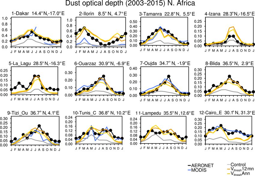
64                                              B. Pu et al.: Retrieving the global distribution of the threshold of wind erosion

Figure 2. (a–i) Frequency distribution of annual mean Vthreshold (black bars) in each region (black boxes in Fig. 1) and Vthreshold for dusty
seasons, i.e., MAM (green) and JJA (blue) for regions in the Northern Hemisphere and SON (orange) and DJF (grey) for regions in the
Southern Hemisphere. The mean (averaged over all grid points in the region, without area weight) and ± 1 standard deviation of Vthreshold
in each region are shown on the top right of each plot.

ble 1 for locations) are shown in Fig. 2a–i. In the Sahel and            short events with a high wind speed. As shown in Table 3,
Sahara, the annual mean Vthreshold peaks around 4 and 4.5–               among the reanalysis wind products tested here, NCEP1 ac-
5.5 m s−1 , respectively (Fig. 2a–b). This magnitude is lower            tually produced a lower Vthreshold in northern Africa than the
than indicated from previous studies based on station ob-                other two reanalyses. Secondly, using the DOD frequency to
servations in the region, e.g., Helgren and Prospero (1987)              approximate dust emission may lead to an overestimation of
found the threshold velocity over eight stations in northwest-           dust emission over regions such as the southern Sahel where
ern Africa ranged from 6.5 to 13 m s−1 during summer in                  transported dust is a large component and consequently an
1974. Chomette et al. (1999) and Marsham et al. (2013) also              underestimation of Vthreshold . Based on our rough estimation,
reported higher wind erosion thresholds around 6–9 m s−1 at              Vthreshold in northern Africa can be underestimated by up to
individual stations. On the other hand, Cowie et al. (2014)              3 m s−1 (Sect. 2.3). In addition, different analysis time peri-
found that the annual threshold of wind erosion at the 25 %              ods or methods to retrieve the wind erosion threshold may
level, i.e., when surface condition is favorable for dust emis-          also contribute to the differences.
sion, can be lower than 6 m s−1 at some sites in the Sahel                  The annual mean Vthreshold in the Arabian Peninsula is a bit
(their Fig. 5). Several factors may contribute to the discrep-           higher, with mean values at 5.2 m s−1 (Fig. 2c). The Vthreshold
ancies. Firstly, studies suggest that reanalysis datasets may            over northern China is even higher, with an annual mean
underestimate surface wind speed in spring and for monsoon               of 7.8 m s−1 . This is consistent with the results of Kurosaki
days in Africa (e.g., Largeron et al., 2015), and therefore they         and Mikami (2007), who found that under favorable land
could lead to a lower value of Vthreshold than that derived              surface conditions the threshold wind speed ranges from
from station observations. In fact, Bergametti et al. (2017)             4.4 ± 0.6 m s−1 in the Taklimakan Desert to 6.9 ± 1.2 m s−1
found even 3-hourly wind speed records at stations may miss              over the Loess Plateau and around 9.8±1.6 m s−1 in the Gobi

Atmos. Chem. Phys., 20, 55–81, 2020                                                           www.atmos-chem-phys.net/20/55/2020/
B. Pu et al.: Retrieving the global distribution of the threshold of wind erosion                                                 65

                                                                        Figure 4. Climatology of annual mean AERONET (a) AOD
                                                                        (550 nm) and (b) SDA COD (500 nm) averaged over 2003–2015.

                                                                        pecially over northern Africa, the Arabian Peninsula, India,
                                                                        and Asia (Fig. 3 and Table 2). The results are thus closer
                                                                        to previous station-based studies over northern Africa. On
                                                                        the other hand, over northern China, Vthreshold is around or
                                                                        greater than 8 m s−1 (Fig. 3e), slighter higher than previ-
                                                                        ous estimates (e.g., Kurosaki and Mikami, 2007; Ginoux and
Figure 3. (a–e) Threshold of wind erosion (Vthreshold ; unit: m s−1 )   Deroubaix, 2017).
derived from satellite products and reanalyses for each season and         In the following section, we will exam if the spatially
the annual mean using DODthresh = 0.5 (or 0.05). Black boxes in         and temporally varying Vthreshold would improve model sim-
(a) denote nine dust source regions as listed in Table 1.               ulation of the DOD spatial pattern, seasonal variations,
                                                                        frequency distribution, and surface dust concentrations in
                                                                        the GFDL AM4.0/LM4.0. Results using Vthreshold with
                                                                        DODthresh = 0.2 (or 0.02) are shown in Sect. 3.2–3.3, and
Desert. These values are also consistent with Ginoux and
                                                                        results using Vthreshold with DODthresh = 0.5 (or 0.05) are
Deroubaix (2017) who found that the regional mean wind
                                                                        briefly discussed in Sect. 4.
erosion threshold over northern China ranges from 6.5 to
9.1 m s−1 . In India, the Vthreshold peaks at about 4.5 m s−1 and
                                                                        3.2     Vthreshold in the GFDL AM4.0/LM4.0 model
6.5 m s−1 , respectively (Fig. 2e). The second peak is proba-
bly related to anthropogenic dust sources over the central In-          In this section we analyze the model output using the default
dian subcontinent (Ginoux et al., 2012). We also note that              setting (Control; Table 4), 12-month (Vthresh 12 mn), and an-
in the Northern Hemisphere, Vthreshold in dusty seasons is              nual mean Vthreshold (Vthresh Ann) by comparing model results
shifted towards lower values than the annual mean (blue and             with multiple observational datasets and MODIS DOD.
green lines in Fig. 2a–f), but it is similar to the annual mean
in the Southern Hemisphere (especially South America and                3.2.1    Climatology of AOD and DOD
Australia), indicating stronger influences of surface variabil-
ity in the Northern Hemisphere.                                         In order to compare the model results with observations, we
   Figure 3 shows the seasonal mean and annual mean global              first show the climatology of AERONET AOD and COD
Vthreshold using DODthresh = 0.5 (or 0.05). The correspond-             from 2003 to 2015. The length of records for each station
ing distribution of annual mean Vthreshold in each region is            is shown in Fig. S6 in the Supplement. As shown in Fig. 4,
shown in Fig. S5 in the Supplement. The derived Vthreshold              annual mean global AOD is highest over Africa, the Arabian
is generally higher than using DODthresh = 0.2 (or 0.02), es-           Peninsula, the Indian subcontinent, and southeastern Asia. In

www.atmos-chem-phys.net/20/55/2020/                                                          Atmos. Chem. Phys., 20, 55–81, 2020
66 B. Pu et al.: Retrieving the global distribution of the threshold of wind erosion Figure 5. Scatter plot of simulated annual mean (a) AOD and (b) COD in the Control run versus AERONET AOD and COD (a, b). The relative difference (as a percentage) (c) between modeled AOD and AERONET AOD and (d) between modeled COD and AERONET COD (c–e). (e) The relative contribution of DOD to COD in the model. the latter two regions, high sulfate concentrations (e.g., Gi- percentage of DOD to total COD in the model is displayed noux et al., 2006) and organic carbon from biomass burning at the bottom (Fig. 5e). The simulated AOD is lower than in southeastern Asia (e.g., Lin et al., 2014) contribute sub- that from AERONET over northern Africa, the Middle East, stantially to the total AOD. The SDA COD shows the optical and western India, largely due to low values of COD sim- depth due to coarse aerosols, which includes both dust and ulated in these regions (Fig. 5d). Besides these regions, the sea salt, and sea salt over coastal regions or islands can be COD over North America, South America, South Africa, and a major contributor. Here, high values (> 0.2) are largely lo- northern Eurasia is also, for the most part, underestimated by cated over dusty regions such as northern Africa, the Arabian the model. Dust is the dominant contributor to the COD value Peninsula, and northern India (Fig. 4b). over most of these low COD regions, except over central-to- Figure 5a–b show the scatter plots of modeled AOD and eastern North America and central South America (Fig. 5e). COD in the Control run versus AERONET AOD and COD, COD (and effectively DOD given its dominance in most respectively. Here column-integrated extinction from both regions) was better simulated in the subsequent model run dust and sea salt is used to calculated COD in the model. The using a prescribed 12-month Vthreshold in terms of both mag- relative differences (as a percentage) between AM4.0 output nitude and spatial pattern. Figure 6 shows the results from the and AERONET station data are also shown (Fig. 5c–d). The Vthresh 12 mn simulation. COD is better captured, while the Atmos. Chem. Phys., 20, 55–81, 2020 www.atmos-chem-phys.net/20/55/2020/
B. Pu et al.: Retrieving the global distribution of the threshold of wind erosion                                           67

Figure 6. Same as Fig. 5 but for the Vthresh 12 mn simulation.

AOD effectively moves from a negative to a slightly positive     tions. The Control run largely underestimates DOD in all re-
bias (Fig. 6a–d). Most sites over northern Africa and the Mid-   gions, while the magnitude of DOD is better captured in the
dle East show a relatively small difference with AERONET         Vthresh 12 mn and Vthresh Ann simulations, although slightly
COD (Fig. 6d). Over the Indian subcontinent, COD is overes-      overestimated in the Sahel and greatly overestimated over
timated, while over North America, excluding the east coast,     Australia. In general, DOD simulated by the Vthresh Ann run
northern Eurasia, and part of South America, COD is also         using a constant annual mean Vthreshold is higher than that
better captured than in the Control run.                         simulated by the Vthresh 12 mn run, consistent with the higher
   These improvements are largely associated with a better       dust emission in the Vthresh Ann run (Table S2 in the Sup-
simulation of DOD in the “dust belt” (i.e., northern Africa      plement). Lack of the soil moisture constraint in the model,
and the Middle East). Figure 7 shows the DOD at 550 nm           which is a very important element in capturing the variation
derived from AERONET AOD (see methodology for details)           of DOD in Australia (Evans et al., 2016), may contribute to
versus that from the Vthresh 12 mn simulation. Over most sta-    the large overestimation of DOD in Australia.
tions in the Sahel, Mediterranean coasts, and central Middle
East, the relative differences between modeled and observed      3.2.2   Climatology of surface dust concentration
DOD is within ±25 %.
   Figure 8 shows the regionally averaged annual mean DOD        While DOD is a key parameter associated with the climate
over nine dusty regions from MODIS and three simula-             impact of dust, surface dust concentration is an important

www.atmos-chem-phys.net/20/55/2020/                                                   Atmos. Chem. Phys., 20, 55–81, 2020
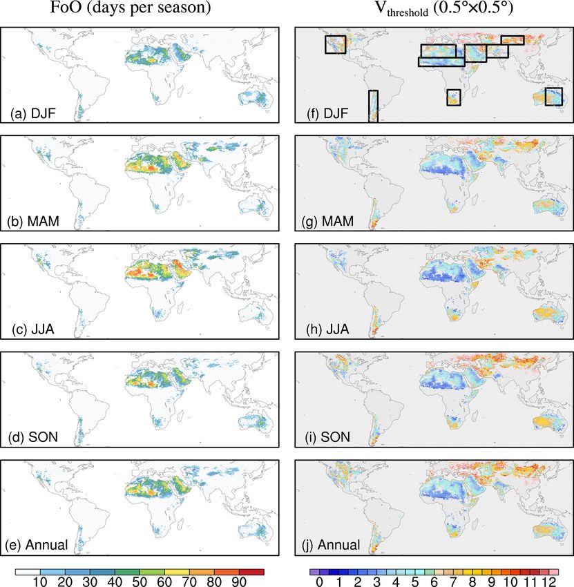
68                                           B. Pu et al.: Retrieving the global distribution of the threshold of wind erosion

Figure 7. (a) Climatology (2003–2015) of AERONET DOD (550 nm) over major dusty regions and (b) scatter plot of modeled DOD in the
Vthresh 12 mn simulation versus AERONET DOD. (c) The relative difference (as a percentage) between modeled DOD and AERONET DOD
in the Vthresh 12 mn simulation.

factor affecting local air quality. Here we compare the mod-       gridded IMPROVE data (Fig. 10). While the Control run
eled surface dust concentration with RSMAS station obser-          largely underestimates surface fine dust concentration, the
vations. Model output is averaged from 2000 to 2015 to form        simulated concentration is overall too high in the Vthresh Ann
the annual climatology. Consistent with the DOD output, the        run. The spatial pattern of fine dust concentration is better
Control run largely underestimates surface dust concentra-         captured in the Vthresh 12 mn run, with higher values over the
tions at almost all of the sites (except sites 9 and 15; Fig. 9,   southwestern US, but the magnitude is still overestimated,
top panel). The underestimation is reduced in the Vthresh Ann      and additional dust hot spots are simulated over the north-
simulation (Fig. 9, middle panel), with seven stations having      ern Great Plains and the Midwest, which are not shown in
model/observation ratios between 0.5 and 2 (white triangles).      the IMPROVE data. Such an overall overestimation may be
Over the coastal US (e.g., sites 16 and 13), dust concentra-       attributed to a lack of soil moisture modulation in the dust
tions are overestimated, consistent with the overestimation        emission scheme. The way in which dust bins are partitioned
of DOD over the US and the Sahel (Fig. 8). Dust concentra-         in the model can add uncertainties to model’s representation
tions in Australia and the east coast of China are also overes-    of surface fine dust concentrations as well. On the other hand,
timated by more than fivefold. Surface dust concentration is       the relatively low spatial coverage of IMPROVE sites over
further improved in the Vthresh 12 mn simulation (Fig. 9, bot-     the northern Great Plains and Midwest (e.g., Pu and Ginoux,
tom), with eight stations showing a model/observation ratio        2018a) may also add uncertainties to the data itself.
between 0.5 and 2 and only four stations overestimating or
underestimating dust concentrations by more than 5 times.
   Simulated surface fine dust concentration (calculated as
dust bin 1 + 0.25× dust bin 2) in the US is compared with

Atmos. Chem. Phys., 20, 55–81, 2020                                                   www.atmos-chem-phys.net/20/55/2020/
B. Pu et al.: Retrieving the global distribution of the threshold of wind erosion                                                  69

                                                                     the Vthresh 12 mn and Vthresh Ann simulations overestimate the
                                                                     DOD by about an order of magnitude.
                                                                        Figure 12 shows the seasonal cycle of COD from 12
                                                                     AERONET SDA sites over northern Africa and nearby is-
                                                                     lands (see Fig. S7 in the Supplement for site locations) along
                                                                     with MODIS DOD and DOD simulated in three runs. The
                                                                     magnitude of AERONET COD and MODIS DOD in these
                                                                     sites are very similar, despite missing values at sites 1, 4,
                                                                     5, 8, and 11 and a smaller value at site 2 in MODIS. Over
                                                                     most of the sites, the seasonal cycle is better captured in the
                                                                     Vthresh 12 mn and Vthresh Ann simulations than the Control run,
                                                                     although the peak over Cairo_EMA_2 (site 12) is slightly un-
                                                                     derestimated, which is consistent with the underestimation of
                                                                     annual mean DOD in the area (Fig. 7).
                                                                        We also examined the seasonal cycle of PM10 surface con-
                                                                     centration at three Sahelian INDAAF stations (see Fig. S7
                                                                     in the Supplement for site locations) from the LISA project.
                                                                     Figure 13a–c show PM10 surface dust concentration (here
                                                                     dust dominates total PM10 concentration) from the Control,
                                                                     Vthresh 12 mn, and Vthresh Ann simulations versus observed
                                                                     PM10 concentrations from three LISA sites. PM10 concen-
                                                                     trations in these sites peak during boreal winter and spring
Figure 8. Regionally averaged annual mean DOD (2003–2015)            and reach minima from July to September. These seasonal
over nine regions from the Control (grey), Vthresh 12 mn (orange),   variations are associated with the dry northerly Harmattan
and Vthresh Ann (yellow) simulations and MODIS (black).              wind in boreal winter and spring that transports Saharan dust
                                                                     southward to the Guinean coast and the scavenging effect of
                                                                     monsoonal rainfall in boreal summer that removes surface
                                                                     dust (Marticorena et al., 2010; Fiedler et al., 2015). While
3.2.3   Seasonal cycles                                              the Control run does not capture the seasonal cycles in these
                                                                     sites, the Vthresh 12 mn run largely captures the spring peak
Figure 11 compares the seasonal cycle of DOD from three              and summer minimum, although the magnitude is overesti-
simulations with MODIS DOD in nine dusty regions. The                mated. In all three sites, the simulated concentration in the
seasonal cycle of gridded AERONET COD (as an approxi-                Vthresh Ann run is larger than that in the Vthresh 12 mn run, es-
mation of DOD; on a 0.5 × 0.5◦ grid) is also shown. Since            pecially from boreal fall to early spring. Such an overestima-
the gridded COD may have large uncertainties over re-                tion is probably due to the prescribed constant annual mean
gions with only a few stations, such as the Sahel, Sahara,           Vthreshold , which is lower than it would be during the less
northern China, and South Africa, MODIS DOD is used as               dusty season (i.e., boreal fall to winter) and thus increases
the main reference in the comparison. Seasonal cycles are            dust emission and surface concentrations.
better captured by the Vthresh 12 mn simulation in the Sa-              Figure 13d–f show the seasonal cycle of DOD from three
hel, the Sahara, and the Arabian Peninsula (Fig. 11a–c), al-         AERONET sites co-located with LISA INDAAF stations
though the spring and summer peak in the Sahel is overes-            and from three simulations. The Vthresh 12 mn and Vthresh Ann
timated, and the winter minimum in the Sahara is underesti-          simulations largely captured the seasonal cycle of DOD at
mated. The MAM peak of MODIS DOD in northern China                   these sites. The overestimation of near-surface PM10 dust
is missed by both Vthresh 12 mn and Vthresh Ann simulations          concentrations (Fig. 13a–c) and the generally well-captured
(Fig. 11d), while the JJA peak over India is largely overes-         column-integrated DOD (Fig. 13d–f) indicate that the model
timated (Fig. 11e). Over the US dusty region, the seasonal           likely underestimates dust concentration in the atmospheric
cycle in the Vthresh 12 mn simulation is slightly underesti-         column above the surface, which needs further investigation
mated compared to MODIS DOD but overestimated from                   in future studies.
May to August in the Vthresh Ann simulation (Fig. 11f). DOD
is underestimated in South Africa in all three simulations           3.2.4   A dust storm over the US northern Great Plains
(Fig. 11g). Over South America, the peak from October to                     on 18 October 2012
February is roughly captured by the Vthresh 12 mn run but is
overestimated by the Vthresh Ann run (Fig. 11h). The seasonal        Can the AM4.0/LM4.0 with the prescribed Vthreshold better
cycles of DOD in Australia are very similar in all three sim-        represent individual dust events? Here we examine a major
ulations and largely resemble that in MODIS, although both           dust storm captured by a MODIS Aqua true color image on

www.atmos-chem-phys.net/20/55/2020/                                                         Atmos. Chem. Phys., 20, 55–81, 2020
You can also read