Mountain-wave-induced polar stratospheric clouds and their representation in the global chemistry model ICON-ART
←
→
Page content transcription
If your browser does not render page correctly, please read the page content below
Atmos. Chem. Phys., 21, 9515–9543, 2021
https://doi.org/10.5194/acp-21-9515-2021
© Author(s) 2021. This work is distributed under
the Creative Commons Attribution 4.0 License.

Mountain-wave-induced polar stratospheric clouds and their
representation in the global chemistry model ICON-ART
Michael Weimer1,2,a , Jennifer Buchmüller2,b , Lars Hoffmann3 , Ole Kirner1 , Beiping Luo4 , Roland Ruhnke2 ,
Michael Steiner5 , Ines Tritscher6 , and Peter Braesicke2
1 Steinbuch   Centre for Computing, Karlsruhe Institute of Technology (KIT), Eggenstein-Leopoldshafen, Germany
2 Institute of Meteorology and Climate Research, Karlsruhe Institute of Technology (KIT),
Eggenstein-Leopoldshafen, Germany
3 Jülich Supercomputing Centre, Forschungszentrum Jülich, Jülich, Germany
4 Institute for Atmospheric and Climate Science, ETH Zurich, Zürich , Switzerland
5 Laboratory for Air Pollution / Environmental Technology, EMPA, Dübendorf, Switzerland
6 Institute of Energy and Climate Research: Stratosphere (IEK-7), Forschungszentrum Jülich, Jülich, Germany
a now at: Department of Earth, Atmospheric and Planetary Sciences, Massachusetts Institute of Technology,

Cambridge, MA, USA
b now at: Steinbuch Centre for Computing, Karlsruhe Institute of Technology (KIT), Eggenstein-Leopoldshafen, Germany

Correspondence: Michael Weimer (michael.weimer@kit.edu)

Received: 5 November 2020 – Discussion started: 19 November 2020
Revised: 22 April 2021 – Accepted: 2 May 2021 – Published: 24 June 2021

Abstract. Polar stratospheric clouds (PSCs) are a driver for    the Antarctic Peninsula nest. We compare a global simula-
ozone depletion in the lower polar stratosphere. They pro-      tion without nesting with the nested configuration to show the
vide surface for heterogeneous reactions activating chlorine    benefits of adding the nesting. Although the mountain waves
and bromine reservoir species during the polar night. The       cannot be resolved explicitly at the global resolution used
large-scale effects of PSCs are represented by means of pa-     (about 160 km), their effect from the nested regions (about
rameterisations in current global chemistry–climate models,     80 and 40 km) on the global domain is represented. Thus, we
but one process is still a challenge: the representation of     show in this study that the ICON-ART model has the poten-
PSCs formed locally in conjunction with unresolved moun-        tial to bridge the gap between directly resolved mountain-
tain waves. In this study, we investigate direct simulations    wave-induced PSCs and their representation and effect on
of PSCs formed by mountain waves with the ICOsahedral           chemistry at coarse global resolutions.
Nonhydrostatic modelling framework (ICON) with its ex-
tension for Aerosols and Reactive Trace gases (ART) in-
cluding local grid refinements (nesting) with two-way in-
teraction. Here, the nesting is set up around the Antarctic     1   Introduction
Peninsula, which is a well-known hot spot for the generation
of mountain waves in the Southern Hemisphere. We com-           Polar stratospheric clouds (PSCs) play a key role in explain-
pare our model results with satellite measurements of PSCs      ing the rapid ozone loss in the polar stratosphere during local
from the Cloud-Aerosol Lidar with Orthogonal Polarization       spring (e.g. Solomon et al., 1986; Solomon, 1999; Braesicke
(CALIOP) and gravity wave observations of the Atmospheric       et al., 2018). Three different types of PSCs or mixtures
Infrared Sounder (AIRS). For a mountain wave event from         thereof can be found in the lower stratosphere: solid nitric
19 to 29 July 2008 we find similar structures of PSCs as well   acid trihydrate particles (NAT), liquid supercooled ternary
as a fairly realistic development of the mountain wave be-      solution droplets (STS) and ice particles (e.g. Peter and
tween the satellite data and the ICON-ART simulations in        Grooß, 2012; Tritscher et al., 2021, and references therein).
                                                                Heterogeneous reactions on the surface of PSCs lead to acti-

Published by Copernicus Publications on behalf of the European Geosciences Union.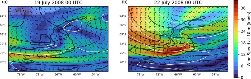
9516                                                     M. Weimer et al.: Mountain-wave-induced PSCs with ICON-ART

vation of chlorine and bromine species during the polar night,   are not able to resolve the full range of mountain waves ade-
thus enhancing the catalytic ozone depletion cycles as soon      quately (Lamarque et al., 2013; Orr et al., 2015; Morgenstern
as the sun rises (e.g. Solomon, 1999). In addition, PSCs can     et al., 2017). Mesoscale models with resolutions as high as
irreversibly remove nitrogen-containing species by sedimen-      7 km have been developed in the past to calculate the local ef-
tation, a process known as denitrification, thus extending the   fect of mountain-wave-induced PSCs (e.g. Fueglistaler et al.,
period of low ozone concentrations during polar spring (e.g.     2003; Eckermann et al., 2006; Plougonven et al., 2008; Noel
Waibel et al., 1999). PSCs may form below specific threshold     and Pitts, 2012), but they need input of a previous simulation
temperatures (e.g. Hanson and Mauersberger, 1988; Marti          of a global model or a reanalysis to provide the boundary
and Mauersberger, 1993; Carslaw et al., 1994), indicating        conditions (e.g. Weimer et al., 2016). Thus, mountain waves
that temperature is a crucial parameter for PSC formation.       and mountain-wave-induced PSCs either have to be parame-
   Mountain waves (orographic gravity waves) are stationary      terised (Orr et al., 2015, 2020; Zhu et al., 2017) or have to be
waves in the lee of a mountain which can develop in a sta-       calculated in a post-processing step via Lagrangian models
bly stratified atmosphere (e.g. Fritts and Alexander, 2003)      (e.g. Mann et al., 2005) or via mesoscale models. An ap-
when a sizeable component of the large-scale flow is perpen-     proach for interactive two-way coupling between the high-
dicular to the mountain range. Mountain waves can propa-         resolution simulations and the global models, in particular
gate upwards into the stratosphere and higher (Wright et al.,    CCMs, is missing so far.
2017) and may perturb the synoptic temperature field with lo-       In this study, mountain-wave-induced PSCs are simulated
cal amplitudes of up to ± 15 K or even more (Carslaw et al.,     seamlessly with the ICOsahedral Nonhydrostatic modelling
1998b; Eckermann et al., 2009; Dörnbrack et al., 2020). In       framework (ICON; Zängl et al., 2015) and its extension for
the polar regions, mountain waves are of particular interest     Aerosols and Reactive Trace gases (ART; Rieger et al., 2015;
for the formation of PSCs because mountain-wave-induced          Weimer et al., 2017; Schröter et al., 2018). ICON-ART pro-
temperature fluctuations can lead to localised cooling that      vides the possibility of local grid refinement (nesting) with
triggers PSC formation even if synoptic-scale temperatures       two-way interaction (see Reinert et al., 2019, for details).
are above the PSC formation temperatures (Carslaw et al.,        Thus, a global low-resolution simulation provides bound-
1998b).                                                          ary conditions for a region with a refined grid, similar to
   Mountain-wave-induced PSCs have a significant influence       mesoscale models. But additionally, the refined grid also
on the ozone depletion over both Antarctica and the Arctic       feeds back to the low resolution, which is a novel approach
(e.g. Höpfner et al., 2006a; McDonald et al., 2009; Alexander    in atmospheric chemistry modelling.
et al., 2011; Hoffmann et al., 2017; Langematz et al., 2018).       We perform a comprehensive case study for a well-
Various regions have been identified from observations and       observed mountain wave event at the Antarctic Peninsula in
models as being hot spots for mountain-wave-induced PSCs,        July 2008 (Noel and Pitts, 2012). We start at a global reso-
such as Greenland and Scandinavia in the Northern Hemi-          lution of about 160 km, which is comparable to other global
sphere and the Southern Andes, the Antarctic Peninsula and       CCMs. We then apply the two-way nesting at the Antarctic
the Transantarctic Mountains in the Southern Hemisphere          Peninsula with a resolution of 40 km in the grid refinement.
(Dörnbrack et al., 2002; Plougonven et al., 2008; Eckermann      This resolution still misses directly resolving gravity waves
et al., 2009; Noel et al., 2009; Hoffmann et al., 2013, 2017).   with horizontal wavelengths lower than about 300 km (cf.
McDonald et al. (2009) estimated that up to 40 % of Antarc-      Geller et al., 2013), but we chose this configuration (1) for
tic PSC formation is associated with mountain waves in the       a balance between accuracy and computational expense and
early Antarctic winter when temperatures are close to the        (2) to show how CCMs could already benefit from modest
NAT formation threshold. Alexander et al. (2013) concluded       higher resolutions. We show how the higher resolution in the
that about 5 % of Antarctic and 12 % of Arctic PSCs are re-      refinement impacts the gravity wave dynamics, PSCs and fi-
lated to mountain wave activity.                                 nally the ozone chemistry in the global model. Thus, this
   Mountain waves are mesoscale features of the atmospheric      study is a first step towards closing the gap between direct
circulation, which poses a challenge for simulating them ex-     simulations of mountain-wave-induced PSC formation and
plicitly with global general circulation models because these    their treatment at coarse global resolutions.
models have limited spatial resolution. The horizontal wave-        We selected the Antarctic Peninsula for this study with the
lengths of mountain waves most relevant for the middle at-       ICON-ART model because it is a well-known hot spot of
mosphere are in the range of tens to hundreds of kilometres      mountain-wave-induced PSCs (Bacmeister, 1993; Bacmeis-
(e.g. Fritts and Alexander, 2003; Eckermann et al., 2006;        ter et al., 1994; McDonald et al., 2009; Alexander et al.,
Orr et al., 2020). Several studies suggest that in a discrete    2011; Hoffmann et al., 2017). Given the strong incident flow
numerical model eight grid points are needed to represent        at low levels and the Antarctic Peninsula protruding a dis-
gravity waves and their dynamics adequately (Geller et al.,      tance of 1300 km with peak heights of up to 2800 m posing
2013; Preusse et al., 2014; Kang et al., 2017). However, cur-    a substantial barrier to this flow, mountain waves with large
rent global chemistry–climate models (CCMs) with horizon-        amplitudes and mesoscale horizontal (> 300 km) and verti-
tal resolutions in the order of a few hundreds of kilometres     cal wavelengths (> 10 km) are typically excited (Alexander

Atmos. Chem. Phys., 21, 9515–9543, 2021                                            https://doi.org/10.5194/acp-21-9515-2021
M. Weimer et al.: Mountain-wave-induced PSCs with ICON-ART                                                                   9517

and Teitelbaum, 2007; Plougonven et al., 2008; Hoffmann               The PSC scheme in ICON-ART calculates ice PSCs based
et al., 2013; Orr et al., 2020). Thus, our ICON-ART model          on the microphysics of the operational configuration at
configuration is expected to be able to capture such waves.        DWD (Doms et al., 2011). For stratospheric temperatures,
   Despite the Antarctic Peninsula being in a remote loca-         the microphysics assumes an ice number concentration of
tion, it is frequently covered by gravity wave and PSC satel-      0.25 cm−3 . Liquid (sulfate and STS) particles are formed by
lite observations, which allows the ICON-ART simulations           the module of Carslaw et al. (1995), with some adaption of
to be evaluated (e.g. Hoffmann et al., 2016; Spang et al.,         the size distributions used. NAT particles are formed by a
2018; Höpfner et al., 2018; Pitts et al., 2018). Here, we          non-equilibrium approach based on Carslaw et al. (2002) and
specifically use Atmospheric Infrared Sounder (AIRS; Au-           van den Broek et al. (2004). The NAT size distribution can
mann et al., 2003; Chahine et al., 2006) and Cloud-Aerosol         be flexibly selected by the model user via XML files (see
Lidar with Orthogonal Polarization (CALIOP; Pitts et al.,          Schröter et al., 2018). A maximum NAT number concentra-
2009, 2018; Höpfner et al., 2009) data to evaluate our simu-       tion of 2.3 × 10⁻⁴ cm−3 is assumed (van den Broek et al.,
lations. AIRS is a cross-track scanning nadir instrument that      2004). The PSC particles are treated separately and exter-
is able to detect stratospheric temperature fluctuations with      nally mixed in each grid box. A detailed description of the
high horizontal resolution (up to 14 km at nadir). Therefore,      PSC scheme can be found in Appendix A.
it is particularly suited to detect the horizontal structures of      While STS particles are calculated diagnostically, NAT
mountain waves in the lower and mid-stratosphere (e.g. Hoff-       particles are separate tracers for each size bin. Both NAT and
mann et al., 2013, 2017). CALIOP, a nadir lidar instrument         ice include prognostic equations that allow the advection of
with high resolution in both a horizontal (5 km) and vertical      these particles into regions with temperatures too large for
(180 m in the lower stratosphere) direction, can detect and        PSC formation, which has been observed in mountain waves
discriminate the different types of PSCs (Pitts et al., 2018).     (Eckermann et al., 2009). The other parts of the scheme are
Therefore, CALIOP is able to identify PSCs formed in moun-         designed similar to global models like the ECHAM/MESSy
tain waves and can be used for the evaluation of PSC schemes       Atmospheric Chemistry model (EMAC; Jöckel et al., 2010;
in models. Sampling the model results on the measurement           Kirner et al., 2011), which have been shown to reflect the
grid of the satellite instruments and converting the data from     main properties of PSCs on a global scale. This study fo-
model quantities to measured quantities (e.g. by means of          cuses on the benefit of increasing the resolution and showing
radiative transfer calculations) is a precise way to evaluate      the impact of the two-way nesting.
the ICON-ART simulations with AIRS and CALIOP obser-                  The chemistry in ICON-ART is based on the Module Effi-
vations (Mishchenko et al., 1996; Grimsdell et al., 2010; Orr      ciently Calculating the Chemistry of the Atmosphere (Sander
et al., 2015).                                                     et al., 2011a), which uses the Kinetic PreProcessor to gener-
   This study is organised as follows: Sect. 2 briefly describes   ate Fortran files for solving the specified chemical mecha-
the ICON-ART model and its PSC scheme. In Sect. 3, the             nism (Sandu and Sander, 2006). Photolysis rates are calcu-
simulation set-up is pointed out that is used to examine the       lated with the CloudJ module (Prather, 2015; Weimer et al.,
mountain wave event at the Antarctic Peninsula. This is fol-       2017). A system of 142 chemical reactions including 38 pho-
lowed by a description of the AIRS and CALIOP instruments          tolytic reactions and 11 heterogeneous reactions on the sur-
in Sect. 4. The model results are compared with CALIOP and         face of PSCs is used. It covers the chemical families Ox ,
AIRS measurements, and the impact of the two-way nesting           HOx , NOx , ClOx , BrOx , a basic hydrocarbon chemistry and
on the chemistry is investigated in Sect. 5. Finally, conclu-      the oxidation of SO2 . The reaction system is similar to other
sions and an outlook follow in Sect. 6.                            studies (e.g. Stone et al., 2019; Zambri et al., 2019; Naka-
                                                                   jima et al., 2020) and can be found in the Supplement. Trace
                                                                   gas emissions at the Earth’s surface are included by a module
2   The ICON-ART model                                             described in Weimer et al. (2017).
                                                                      The model equations of ICON-ART are discretised hori-
The ICON model is the operational model for numerical              zontally on an icosahedral-triangular C grid (e.g. Staniforth
weather prediction at the German Weather Service (DWD;             and Thuburn, 2012; Zängl et al., 2015). The global resolution
Zängl et al., 2015). In addition, it can be applied to large       can be refined by root divisions and bisections of the original
eddy simulations (Dipankar et al., 2015) and fully coupled         icosahedron, resulting in the horizontal resolution descrip-
with an ocean and a land surface model for climate integra-        tion RnBk, as defined by e.g. Zängl et al. (2015). Vertical
tions with the climate physics configuration (Giorgetta et al.,    discretisation is performed on generalised smooth-level co-
2018). The ART extension has been developed to incorporate         ordinates (Leuenberger et al., 2010).
aerosols and the atmospheric chemistry into ICON. It can              For the purpose of detailed simulations around a specific
be coupled to ICON in configurations for numerical weather         region, the grid can be refined for the area of interest by fur-
prediction (Rieger et al., 2015) and allows flexible configu-      ther bisections. Here, the parent domain provides boundary
rations for weather and climate integrations (Schröter et al.,     conditions for the nested domain. The simulated values in
2018).                                                             the nested domain are interpolated to the parent grid with

https://doi.org/10.5194/acp-21-9515-2021                                            Atmos. Chem. Phys., 21, 9515–9543, 2021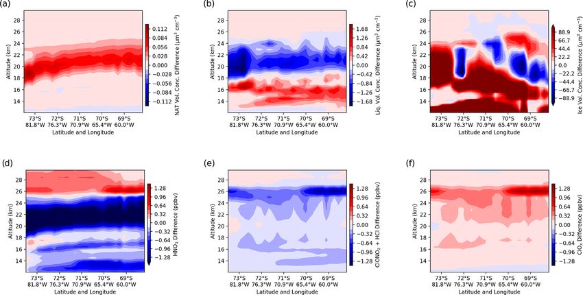
9518                                                       M. Weimer et al.: Mountain-wave-induced PSCs with ICON-ART

a relaxation-based method (Reinert et al., 2019). Thus, the           The emission datasets used in this study are summarised in
global domain is nudged towards the values in the nests,           Table 2. Emissions of CH4 , CO, CO2 , N2 O, SO2 and CFCl3
which will be further investigated in Sect. 5.                     are considered. The Global Emission Inventories Activity
                                                                   (GEIA) dataset for chlorofluorocarbons (CFCs) provided by
                                                                   the Emissions of atmospheric Compounds and Compilation
3   Simulation with nests around the Antarctic Peninsula           of Ancillary Data database (ECCAD) includes only the year
                                                                   1986 and should eventually be adapted by the online emis-
In 2008, a mountain wave event took place between 19               sion tool by Jähn et al. (2020) for the simulated year. Since
and 29 July around the Antarctic Peninsula (Noel and Pitts,        the emission rates of CFCl3 have decreased by more than
2012), which is further investigated in this study. A three-step   40 % since 1986 (Montzka et al., 2018), we neglect the emis-
simulation is conducted; see Fig. 1.                               sions of other CFCs for the less than 1-year simulation. In
   In the first step, the simulation starts on 1 March 2008 with   combination with the emission tool by Jähn et al. (2020) and
a global resolution of R2B04 (1x of about 160 km) as a free-       in the context of the recently found source of CFCs (Montzka
running simulation until 1 May 2008. The first of March is         et al., 2018; Lickley et al., 2020), further CFCs should be
chosen because almost no PSCs are formed at this time either       considered in future simulations.
in the Northern or in the Southern Hemisphere (Tully et al.,          NAT PSCs are simulated using a size distribution based
2011). This period is used as a spin-up period for the chem-       on van den Broek et al. (2004), shown in Fig. 3. We pre-
istry until the southern hemispheric polar vortex intensifies      scribe H2 SO4 in the lower stratosphere (Thomason et al.,
(Schoeberl and Newman, 2003), and PSCs formed in 2008              2008; SPARC, 2013) in the global domain. In the nested do-
(Tully et al., 2011).                                              mains, H2 SO4 runs freely after being initialised by the parent
   In the second step, the meteorological variables are re-        domain.
initialised every second day by the reanalysis product of
ECMWF, ERA-Interim (Dee et al., 2011), in the period be-
tween 1 May and 18 July 2008, but the chemical tracers are         4     Satellite datasets
free-running. This ensures a comparable evolution of the po-
lar vortex in the model with respect to the reanalysis. This       4.1    CALIOP
method was already introduced e.g. in Schröter et al. (2018).
   In the third step, we conducted two simulations covering        The Cloud-Aerosol Lidar with Orthogonal Polarisation
the mountain wave event from 19 to 29 July 2008: one sim-          (CALIOP; Pitts et al., 2009, 2018; Höpfner et al., 2009) on
ulation without any nests and one simulation with two-way          board the Cloud-Aerosol Lidar and Infrared Pathfinder Satel-
nesting around the Antarctic continent (R2B05, 1x of about         lite Observation (CALIPSO) was launched on 28 April 2006
80 km) and around the Antarctic Peninsula (R2B06, 1x of            (Winker et al., 2007). In 2008, the satellite flew as part of
about 40 km); see Fig. 2 and Table 1. The chemistry – in-          NASA’s A-Train constellation in an orbit with 98◦ inclina-
cluding PSCs, photolysis and transport of tracers – is calcu-      tion at an altitude of 705 km (Stephens et al., 2002; Pitts et al.,
lated in all domains. Since we are interested in the interac-      2018). Its orbit was sun-synchronous with Equator crossings
tion between the model domains, we decided to avoid every          at about 01:30 and 13:30 LT. It measured down to 82◦ S with
influence by other models during this part of the simulation,      a repeat cycle of 16 d. In February 2018, it was moved to a
and hence they are free-running. Output in this third step of      lower orbit.
the simulation is given (1) at the specific Antarctic Penin-          CALIOP is a light detecting and ranging (lidar) instru-
sula overpasses of AIRS for the Antarctic Peninsula nest and       ment, set up in nadir geometry. It scans the atmosphere at
(2) hourly during the whole period of the mountain wave            wavelengths of 532 and 1064 nm with parallel and orthog-
event.                                                             onal polarisations for the 532 nm channel (Winker et al.,
   On 1 March 2008, the meteorological variables are ini-          2007). At altitudes from 8.4 to 30 km, the vertical resolution
tialised with ERA-Interim. The chemical tracers are ini-           is 180 m or higher. Horizontal averaging of 5 km is applied
tialised by an EMAC simulation which included tropospheric         for the detection of PSCs with CALIOP (Pitts et al., 2018).
as well as stratospheric chemistry similar to Jöckel et al.        At the Earth’s surface, the light beam has a diameter of about
(2016). Sea surface temperature and sea ice cover are based        100 m (Höpfner et al., 2009; Pitts et al., 2018).
on monthly varying values of the climatology by Taylor et al.         For the detection of PSCs, a combination of two values is
(2000), linearly interpolated to the simulation date. The ad-      used (Pitts et al., 2018): (1) the ratio of total and molecular
vective model time step is set to 360 s. Vertically, the same 90   backscatter coefficient R532 and (2) the backscatter coeffi-
levels are used as in the operational set-up of DWD weather        cient at perpendicular polarisation β⊥ , both at a wavelength
forecasts, covering the altitude range from the surface up to      of 532 nm. Discrimination of the PSC types can be seen in
75 km (see e.g. Weimer et al., 2017, Fig. 1). In the lower         diagrams of R532 vs. β⊥ . Different regions in this diagram
stratosphere, the vertical grid spacing increases from 400 m       refer to the different PSC categories: STS, NAT mixtures,
at an altitude of 12 km up to about 1200 m at 30 km.               enhanced NAT mixtures, ice and wave ice (see Pitts et al.,

Atmos. Chem. Phys., 21, 9515–9543, 2021                                               https://doi.org/10.5194/acp-21-9515-2021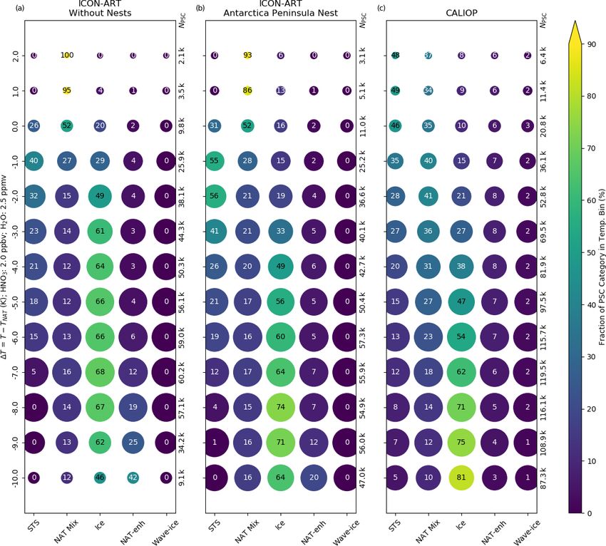
M. Weimer et al.: Mountain-wave-induced PSCs with ICON-ART                                                                            9519

Figure 1. Simulation set-up in this study: a free-running simulation from 1 March until 30 April 2008 is followed by a period until 18
July 2008 where the meteorology is re-initialised every second day. During the mountain wave event until 29 July 2008, two simulations
are performed: one global simulation without nests (with 160 km resolution) and one simulation with the nests (with 160, 80 and 40 km
resolution) as visualised in Fig. 2 including two-way nesting.

Table 1. Overview of the simulation set-up for the investigation of the mountain wave event in July 2008. For details see text.

                  Time period (in 2008)     Resolution    Output interval (h)     Remark
                  1 March–30 April          R2B04                           24    Spin-up for chemistry, free-running
                  1 May–18 July             R2B04                           24    Dynamics re-initialised every second day
                  19–29 July                R2B04                             1   Free-running
                                            see Fig. 2                 see text   Including two-way nesting

Figure 2. Visualisation of the nested domains used in the simula-
tion with the nests: a global resolution of R2B04 (1x ≈ 160 km) is
used, with the first circular refined grid around the Antarctic con-
tinent (R2B05, 1x ≈ 80 km) and a second rectangular refinement
around the Antarctic Peninsula (R2B06, 1x ≈ 40 km). The white
line shows the location of the cross section analysed in Sect. 5.3.

                                                                          Figure 3. Size distribution of NAT particles used in this study.
2018). The thresholds to distinguish PSCs from background
                                                                          Based on van den Broek et al. (2004).
noise are calculated as daily median plus 1 absolute standard
deviation and depend on potential temperature (β⊥,thres and
R532,thres ). Particles with β⊥ < β⊥,thres and R532 > R532,thres
are attributed to the STS category. If β⊥ > β⊥,thres , non-               all, the classification scheme has been shown to be applicable
spherical particles are assumed. Pitts et al. (2018) estimated            to ground-based lidars with comparable results (Snels et al.,
that 10 % to 15 % of particles classified as NAT mixtures and             2019) and has been shown to be in the expected thermody-
STS could be misclassified and may lead to enhancements in                namic existence regimes (Pitts et al., 2018).
the respective other class. The boundary between the NAT                     We use the PSC climatology of Pitts et al. (2018), which is
mixtures and ice (RNAT|ice ) is calculated dynamically de-                the version 2 level 1B data. It is restricted to night-time south-
pending on the state of dehydration and denitrification (Pitts            ern hemispheric data during the mountain wave event (data
et al., 2018). The category of enhanced NAT mixtures repre-               are available within the time frame we are interested in from
sents NAT particles nucleated heterogeneously on wave ice                 22 to 29 July 2008). We examine the altitude levels between
PSCs. Both the enhanced NAT mixtures and wave ice cate-                   15 and 30 km where (1) no tropospheric clouds contaminate
gories depend on empirically set thresholds of β⊥ and R532                the results and (2) most of the PSCs can be found (see e.g.
and therefore are not “all-inclusive” (Pitts et al., 2018). Over-         Fig. 13 of Pitts et al., 2018). In addition, the dataset includes

https://doi.org/10.5194/acp-21-9515-2021                                                    Atmos. Chem. Phys., 21, 9515–9543, 2021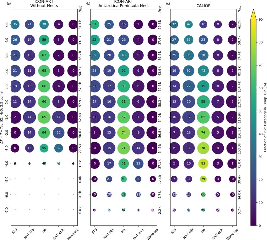
9520                                                                     M. Weimer et al.: Mountain-wave-induced PSCs with ICON-ART

Table 2. Emission datasets used in this study.

                            Species       GEIAa         MACCityb           MEGAN-MACCc                  GFED3d          EDGARv4.2e
                            CH4               –               X                       X                      X                  –
                            CO                –               X                       X                      –                  X
                            CO2               –               –                       –                      X                  X
                            N2 O              –               –                       –                      X                  X
                            SO2               –               X                       –                      X                  –
                            CFCl3             X               –                       –                      –                  –
                          a Cunnold et al. (1994). b van der Werf et al. (2006); Lamarque et al. (2010); Granier et al. (2011); Diehl et al.
                          (2012). c Sindelarova et al. (2014). d van der Werf et al. (2010). e Janssens-Maenhout et al. (2011, 2013).

temperature and pressure data of Modern-Era Retrospective                              5     Mountain-wave-induced PSCs with ICON-ART
analysis for Research and Applications version 2 (MERRA2;
Gelaro et al., 2017), which originally has a horizontal reso-                          Here, we investigate a mountain wave event during July 2008
lution of 0.5◦ × 0.625◦ , interpolated on the CALIOP paths.                            with ICON-ART in a configuration with interactive chem-
                                                                                       istry and local grid refinement around the Antarctic Penin-
4.2    AIRS                                                                            sula. This section comprises an evaluation of the dynamical
                                                                                       structure of the mountain wave with AIRS (Sect. 5.1) and
The Atmospheric InfraRed Sounder (AIRS; Aumann et al.,                                 comparisons of the model results with CALIOP measure-
2003; Chahine et al., 2006) is one of the instruments on                               ments (Sect. 5.2). In addition, it discusses the impact of the
board the Aqua satellite, which was launched in May 2002                               direct simulation of mountain-wave-induced PSCs on the po-
and which is part of the A-Train constellation right ahead of                          lar ozone chemistry (Sect. 5.3).
CALIPSO. Thus, its orbit is the same as CALIPSO in 2008
but about 1 to 2 min ahead of CALIPSO1 .                                               5.1     Near-surface meteorological conditions and
   The AIRS instrument is a nadir sounder with across-track                                    stratospheric dynamical structure of the mountain
scanning capabilities that scans the atmosphere by 90 foot-                                    wave
prints per scan with a ground coverage of 1780 km and a
size of 13.5 × 13.5 km2 (nadir) to 41 × 21.4 km2 (scan edge)                           The evolution of the ozone loss and the Antarctic polar vor-
per footprint (e.g. Orr et al., 2015; Hoffmann et al., 2017).                          tex in 2008 was comparable to the previous years although
It measures the spectrally resolved radiances in wavelengths                           the so-called ozone hole lasted rather long into December
between 3.74 and 15.4 µm. Brightness temperatures (BTs) in                             (Tully et al., 2011). It was a year with increased gravity wave
the 15 µm band can be used to derive information about grav-                           activity at the Antarctic Peninsula (Hoffmann et al., 2016).
ity waves in the lower polar stratosphere (Hoffmann et al.,                            We chose a gravity wave event lasting 10 d from 19 until 29
2017). In this study we use a data product averaging over 21                           July 2008 with lowest temperatures during the whole winter
channels around 15 µm to improve the signal-to-noise ratio                             season (Noel and Pitts, 2012). By end of July 2008, the po-
(Hoffmann et al., 2017). The temperature weighting function                            lar vortex was close to its maximum extension, whereas the
in this band peaks at an altitude of around 23 km with a full                          stratospheric ozone concentration started to decrease (Tully
width at half maximum of 15 km and with information from                               et al., 2011).
the altitude range between 17 and 32 km. Therefore, it is well                            Figure 4 summarises the large-scale meteorological condi-
suited to derive information about gravity waves in the alti-                          tions around the peninsula, based on the ERA-Interim reanal-
tude region where PSCs are expected to exist.                                          ysis. As indicated e.g. by Alexander and Teitelbaum (2007),
   This band is used to examine the mountain wave event                                the ability of ERA-Interim to capture mesoscale mountain
at the Antarctic Peninsula mentioned above. The same algo-                             wave events is limited. Therefore, we use the reanalysis
rithm as in previous studies is used to compare the model data                         to show the meteorological background conditions and will
with specific Antarctic Peninsula overpasses of AIRS (Hoff-                            evaluate the lower-stratospheric temperature perturbations
mann and Alexander, 2010; Hoffmann et al., 2016, 2017). In                             with AIRS later in this section. Figure 4 shows several vari-
particular, the ICON-ART data are resampled on the AIRS                                ables at the beginning of the mountain wave event on 19 July
measurement grid, and a radiative transfer model is used to                            2008 (panel a) and around its peak dynamics on 22 July 2008
simulate AIRS measurements based on the ICON-ART data                                  (panel b). Panels covering the whole event can be found in
to allow for a direct comparison with the real observations.                           the Supplement (Fig. S1).
                                                                                          The Antarctic Peninsula was located at the vortex edge
   1 https://www-calipso.larc.nasa.gov/about/atrain.php (last ac-                      during the whole mountain wave event, as depicted by the
cess 19 March 2021)                                                                    shaded regions in the panels and determined by the method

Atmos. Chem. Phys., 21, 9515–9543, 2021                                                                          https://doi.org/10.5194/acp-21-9515-2021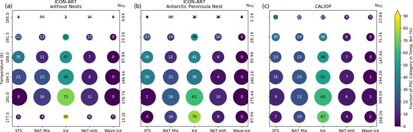
M. Weimer et al.: Mountain-wave-induced PSCs with ICON-ART                                                                               9521

Figure 4. Meteorological situation at the Antarctic Peninsula for (a) 19 and (b) 22 July 2008 at 00:00 UTC from ERA-Interim. The colours
and the wind barbs depict the surface wind in knots. The white lines correspond to the mean sea level pressure in hectopascals. The black lines
are geopotential heights at 500 hPa in geopotential decametres. The shaded regions show the air masses within the polar vortex, determined
according to Nash et al. (1996) on θ = 475 K. Panels covering the whole period of the mountain wave event can be found in the Supplement.

by Nash et al. (1996). Starting from 19 July 2008, an ap-                 Peninsula nest can capture the main features of the mountain
proaching high-pressure system led to an increase of the                  wave.
mean sea level pressure gradient (white lines) at the Antarctic              Fine structures such as in panel j of Fig. 5 cannot be simu-
Peninsula with a corresponding increase of easterly winds at              lated in this simulation set-up of ICON-ART (e.g. panel k)
the mountain range (wind barbs and colour-coded). The gra-                since the resolution of 40 km is still too coarse to predict
dient on the geopotential height at 500 hPa (black lines) was             them, which was already indicated by the comparison to
also increased, showing the large-scale easterly flow at this             CALIOP. This might be a resolution issue which would
altitude on 22 July.                                                      perhaps be improved by going to higher grid spacings, as
   These conditions led to a mountain wave event lasting for              shown by Orr et al. (2015). The chemistry non-linearly de-
10 d, which is now compared to AIRS measurements. For                     pends on temperature, which means that small temperature
this, temperature and pressure of ICON-ART in the Antarc-                 variations could have a measurable effect on the chemistry
tic Peninsula nest are saved at the time step closest to each             (e.g. Murphy and Ravishankara, 1994). As pointed out pre-
of the AIRS overpasses during 20 and 21 July 2008. These                  viously, the microphysics of PSCs are one example for this.
data are then convolved with the same temperature weight-                 If the amplitude is underestimated, like in Fig. 5b and c, a
ing functions that apply for the AIRS observations (see e.g.              more highly resolved model would most probably generate
Hoffmann et al., 2017). The same methodology was applied                  more ice PSCs, thus improving the CALIOP comparison at
to model simulations by Orr et al. (2015). The resulting BT               the lowest temperatures; cf. e.g. Figs. 5 to 7 of Orr et al.
perturbations can be found in Fig. 5 on 20 July and in Fig. 6             (2020), who used a higher-resolution simulation to parame-
on 21 July 2008 for AIRS and ICON-ART.                                    terise mountain-wave-induced PSCs.
   Horizontal structures of the BT perturbations are shown in                These results are also stressed by the comparison of the
the first and second columns for AIRS and ICON-ART, re-                   perturbations at the latitude of 70◦ S that are shown in the
spectively. Largest perturbations are present directly above              third column of Figs. 5 and 6. The largest BT perturbations
the Antarctic Peninsula for both AIRS and ICON-ART,                       can be found at the longitude of the Antarctic Peninsula in all
which demonstrates that the perturbations originate from                  the panels. Some fine structures are missing in ICON-ART.
mountain waves propagating into the lower stratosphere. In                For instance, at some overpasses the amplitude of the wave
addition, the mountain wave has an angle with respect to the              is underestimated compared to AIRS (e.g. panel c of Fig. 6).
Antarctic Peninsula mountains of about 45◦ , represented in               An analogous study by Orr et al. (2015) using a 4 km reso-
both AIRS and ICON-ART. The horizontal wavelength of the                  lution seems to suggest a better match between model and
simulated mountain wave is in the order of 300 km, which is a             observations. At other overpasses, the phase of the wave is
medium–large wavelength compared to other events (see e.g.                shifted with respect to AIRS, such as in panel c of Fig. 5 and
Alexander and Teitelbaum, 2007; Plougonven et al., 2008;                  panel f of Fig. 6. This is most probably a result of the free-
Hoffmann et al., 2014). Therefore, the ICON-ART simula-                   running simulation where the wave cannot be expected to be
tion with lower-stratospheric vertical resolution in the order            located at exactly the same location as in the measurements.
of 500 m and horizontal resolution of 40 km in the Antarctic                 In total, the comparison with AIRS showed that, apart
                                                                          from some missing fine structures, the mountain wave event

https://doi.org/10.5194/acp-21-9515-2021                                                    Atmos. Chem. Phys., 21, 9515–9543, 2021
9522 M. Weimer et al.: Mountain-wave-induced PSCs with ICON-ART Figure 5. Comparison of AIRS and ICON-ART brightness temperature (BT) perturbations at wavelengths of 15 µm for all Antarctic Peninsula overpasses of AIRS during 20 July 2008. The first column shows the BT perturbation observed by AIRS, and the second column the simulated perturbation based on ICON-ART in the Antarctic Peninsula nest. The third column shows the perturbation for AIRS (black) and ICON-ART (orange) at a latitude of 70◦ S. The rows show different overpasses at (a–c) 03:49 UTC, (d–f) 05:28 UTC, (g–i) 18:55 UTC and (j–l) 20:33 UTC. Atmos. Chem. Phys., 21, 9515–9543, 2021 https://doi.org/10.5194/acp-21-9515-2021
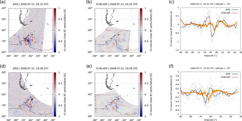
M. Weimer et al.: Mountain-wave-induced PSCs with ICON-ART                                                                     9523

Figure 6. Same as Fig. 5 but for 21 July 2008. The rows show different overpasses at (a–c) 04:32 UTC and (d–f) 19:38 UTC.

taking place in the end of July 2008 can be represented with          is also consistent with previous studies of mountain waves
the resolution of 40 km in comparison with AIRS. In the fol-          (Meilinger et al., 1995; Carslaw et al., 1998a; Eckermann
lowing, we will analyse how this directly simulated mountain          et al., 2009).
wave event impacts the dynamics in the coarser-resolution                The relatively large temperature gradients in the Antarc-
domains in ICON-ART.                                                  tic Peninsula nest are also in agreement with gradients in the
   Figure 7 shows cross sections of the mountain wave dy-             wind velocities, which are shown in the second and third row
namics along the line shown in Fig. 2 for the example of 22           of Fig. 7. In the lee of the Antarctic Peninsula, the vertical
July 2008 at 04:00 UTC in the altitude range between 12 and           wind velocity changes signs at altitudes where the tempera-
30 km. The model data are interpolated to the path by an in-          ture increases or decreases and has maximum values above
verse distance method including the three neighbouring grid           0.3 m s−1 . Largest horizontal wind velocities in the order of
points. The left column shows the simulation without nests,           75 m s−1 occur at altitudes above 27 km.
whereas the three other columns illustrate the dynamics in               The mountains also cause perturbations in the potential
the different domains shown in Fig. 2 of the simulation with          temperature (fourth row in Fig. 7) in the lee. If diabatic pro-
the nests.                                                            cesses are negligible, the flow follows the contours of poten-
   The bottom row of Fig. 7 shows the resolution of the               tial temperature, which will be shown in the PSC precursors
Antarctic Peninsula in the different domains. As can be seen,         in Sect. 5.3.2.
the higher the horizontal resolution, the better the Antarctic           Up to now, it was only demonstrated that this mountain
Peninsula can be represented as mountain range. Thus, this            wave event can be directly simulated in the Antarctic Penin-
indicates that the interaction between the flow and the de-           sula nest (right column), compares well to measurements and
tailed orography in the Antarctic Peninsula nest is improved          is consistent with the theory of mountain waves (Queney,
with respect to the global resolution of 160 km.                      1947; Smith, 1989). In addition, Fig. 7 also shows the im-
   This is reflected in the variables shown in Fig. 7. Temper-        pact of the two-way nesting in ICON-ART. The nest around
atures close to 175 K only occur in the Antarctic Peninsula           Antarctica with a resolution of about 80 km (third column)
nest with a 40 km resolution in the lee of the mountain. The          interacts with both nests and shows the transition between
temperature in the Antarctic Peninsula nest also shows the            these resolutions. The mountain wave at the Antarctic Penin-
characteristic high- and low-temperature patterns as calcu-           sula cannot be represented adequately at the resolution of
lated in theory (e.g. Queney, 1947; Smith, 1989) and seen             160 km in the simulation without the nests (left column in
in measurements (e.g. Wright et al., 2017). As already indi-          Fig. 7). The characteristic wave patterns do not occur in this
cated by Figs. 5 and 6, the temperature perturbation in the           simulation. In contrast to this, the global domain in the sim-
order of 10 K compares well to the AIRS measurements and              ulation with the nests (second column in Fig. 7) shows a de-

https://doi.org/10.5194/acp-21-9515-2021                                               Atmos. Chem. Phys., 21, 9515–9543, 2021
9524                                                          M. Weimer et al.: Mountain-wave-induced PSCs with ICON-ART

Figure 7. Cross sections on 22 July 2008 at 04:00 UTC along the white line in Fig. 2. Each row represents a different variable in the model.
The bottom row shows the surface altitude with the Antarctic Peninsula at around 65◦ W. The columns represent the different simulations
and domains: the first column is the simulation without nests (1x ≈ 160 km); the second one is the global domain (1x ≈ 160 km) including
two-way nesting; and the two right columns represent the Antarctica (1x ≈ 80 km) and Antarctic Peninsula nests (1x ≈ 40 km), respectively.
The dynamical variables temperature, vertical wind velocity, horizontal wind velocity and potential temperature are shown in this figure.

crease in temperature of about 2 K in the lee of the moun-                 This is also visible in the other variables of Fig. 7. Espe-
tains. This is a result of the two-way nesting and the lower            cially for the vertical wind velocity (second row), one can see
temperature due to the directly simulated mountain wave in              that wave-like structures occur in the global domain where
the Antarctic Peninsula nest. The amplitude is lower than it is         they cannot be represented without the nests. Therefore, we
expected by mountain waves, but the effect of the mountain              can expect that mountain-wave-induced PSCs can also be
wave is still remarkable, even in the global grid of 160 km             represented at this relatively low global resolution because
resolution.                                                             they are directly simulated in the locally refined regions. In
                                                                        the following section, we will compare PSCs to CALIOP

Atmos. Chem. Phys., 21, 9515–9543, 2021                                                    https://doi.org/10.5194/acp-21-9515-2021
M. Weimer et al.: Mountain-wave-induced PSCs with ICON-ART 9525
measurements in the Antarctic Peninsula nest before we anal- bins. The data are restricted to the region of the Antarctic
yse the impact of further model variables on the chemistry. Peninsula nest resulting in a total number of about 1 million
grid points with PSCs for CALIOP and about 0.5 million grid
5.2 Comparison of simulated PSCs with CALIOP points with PSCs in ICON-ART. This large difference could
measurements be either a result of horizontally shifted PSCs, especially in
the later part of the free-running simulation, or a problem
For a comparison with CALIOP, the ICON-ART PSC vol- with the constant number concentrations used in the model.
ume concentrations are interpolated (1) horizontally by an It should be further analysed in the future.
inverse distance method, (2) linearly in time and (3) linearly Figure 8 shows the relative number of grid points (in per
in geometric altitude to all CALIOP paths from 22 to 29 cent) on the CALIOP paths where the different PSC cate-
July 2008 where CALIOP’s orbit was within the region of gories occur. The size of the circles corresponds to the total
the Antarctic Peninsula nest. Details about the interpolation number of grid points with PSCs, and the colour of the cir-
can be found in Weimer (2019, Sect. 4.7.4). cles shows the relative number of this PSC category occur-
As pointed out by previous studies, an adequate compar- rence in the respective temperature bin. The panels show the
ison of CALIOP with model data can only be set up if the PSC occurrence (a) in the simulation without the nests, (b) in
model data are transferred into the optical space measured the Antarctic Peninsula nest and (c) in the CALIOP mea-
by CALIOP at 532 nm. We apply the method by Engel et al. surements. For ICON-ART (panels a and b), the modelled
(2013), Tritscher et al. (2019) and Steiner et al. (2021). It temperatures are used directly. The temperature for CALIOP
is based on T-matrix and Mie calculations (e.g. Mishchenko (panel c) is interpolated from MERRA2 and provided as part
et al., 1996) with particle number densities and particle radii of the original dataset (Pitts et al., 2018).
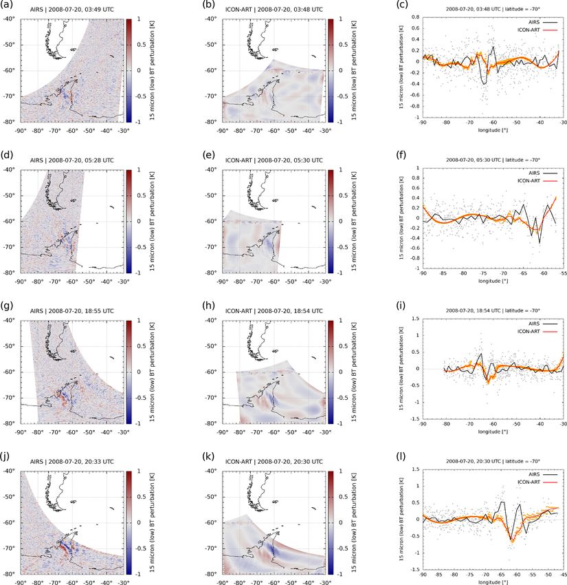
of the PSC types as input. The external PSC mixtures of As can be seen, the relative distribution of grid points with
ICON-ART are combined to optical properties (R532 and β⊥ ) PSCs coincides in all panels down to a temperature of about
for each grid point. In accordance with Tritscher et al. (2019) 180 K. Temperatures lower than that, however, are under-
and Steiner et al. (2021) we use aspect ratios of ice and NAT represented in the simulation without the nest, compared to
of 0.9 and refractive indices of 1.44 for STS (Krieger et al., CALIOP. This is expected from Fig. 7 since temperatures are
2000), 1.31 for ice and 1.48 for NAT (Middlebrook et al., higher than 180 K in the simulation without nests in the lee
1994). of the mountains. In addition, the simulation without nests
The three thresholds to determine the boundaries between overestimates the fraction of the ice category at temperatures
the PSC categories, as mentioned in Sect. 4.1, are taken from lower than 183 K compared to CALIOP.
the measurement data and averaged daily for each CALIOP Both deficiencies are improved in the Antarctic Peninsula
height level (β ⊥,thres , R 532,thres and R NAT|ice ) (Tritscher et al., nest with a resolution of 40 km (panel b). PSCs in the ice
2019; Steiner et al., 2021). As pointed out by Engel et al. category occur with a similar fraction like in CALIOP in the
(2013), it is important to account for the measurement un- 181 K bin, and the relative number of grid points with PSCs
certainties σR and σβ,⊥ to compare the simulated R532 and in the lowest temperature bin coincides with the measure-
β⊥ with CALIOP. These uncertainties are calculated accord- ments. The fractions of the NAT mixtures and enhanced NAT
ing to Eqs. (5) and (6) of Tritscher et al. (2019), respectively. categories are also comparable to CALIOP over the whole
The simulated R532 and β⊥ are scaled by a normal distribu- range of temperatures. For medium temperatures (188 and
tion with mean at the simulated value and standard deviation 184.5 K) the fraction of the STS category is slightly over-
as the respective σ . To summarise, the condition to determine estimated compared to CALIOP. A reason for this could be
if a PSC is detected is then missing fine structures in the gravity wave, as already indi-
2 cated by Figs. 5 and 6. The fraction of the ice category is 9 %
βscal > β ⊥,thres + σβ,⊥ , βscal ∼ N (β⊥ , σβ,⊥ ) (1)
larger in the lowest temperature bin than in CALIOP.
or Although Fig. 7 suggests that main parts of the moun-
R532,scal > R 532,thres + σR , R532,scal ∼ N R532 , σR2 . (2) tain wave can be captured in the Antarctic Peninsula nest,
no PSCs in the “wave ice” category are simulated by ICON-
Since the ICON-ART simulations are free-running, we ART. As mentioned in Sect. 2, the ice particle number con-
cannot expect the PSCs to occur at exactly the same locations centration is essentially set to the constant value of 0.25 cm−3
as in the measurements. Therefore, we compare the evolution in the stratosphere. The ice number concentration in moun-
of PSCs with respect to the temperature in both CALIOP and tain waves can increase to values of a few cubic centime-
ICON-ART, which is a crucial parameter in the formation of tres and then lead to larger backscatter ratios (e.g. Engel
PSCs (e.g. Solomon, 1999). We count the occurrence of the et al., 2013). Therefore, this too-low ice number concentra-
different PSC categories by the method described above in tion could explain why the backscatter ratio for determin-
temperature bins and compare them between ICON-ART and ing the PSC categories does not get as large as 50, which is
CALIOP. The “no” PSC category is neglected in this compar- needed for the wave ice category (Pitts et al., 2018). On the
ison to emphasise the occurrence of PSCs in the temperature other hand, as mentioned in Sect. 4.1, the wave ice category
https://doi.org/10.5194/acp-21-9515-2021 Atmos. Chem. Phys., 21, 9515–9543, 20219526 M. Weimer et al.: Mountain-wave-induced PSCs with ICON-ART
Figure 8. Statistical analysis of PSC occurrence for (a) the ICON-ART simulation without nests, (b) the ICON-ART simulation with nests in
the Antarctic Peninsula nest and (c) CALIOP measurements. The data are restricted to the region of the Antarctic Peninsula nest for all panels
to get comparable results. The ICON-ART data are interpolated to the CALIOP paths in the altitude range from 15 to 30 km in the nest in the
time range between 22 and 29 July 2008 where CALIOP data are available. The colours correspond to the numbers in the circles and show
the fraction of the PSC category that is present in the temperature bins with a width of 3.5 K. The sizes of the circles correspond to the total
number of grid points with PSCs in the temperature bins relative to the maximum in each panel, also denoted on the right-hand side of the
panels as NPSC , following the nomenclature by Spang et al. (2016). The “k” behind the numbers abbreviates thousand; i.e. 179.7 k = 179 700
grid points with PSCs. The temperature data for CALIOP originate from MERRA2, which is part of the CALIOP product.
is based on an empirical threshold of R532 > 50, so that parts As can be seen in Fig. 9, the number of grid points with
of the wave ice clouds could also be attributed to the ice cat- PSCs grows when the temperature gets lower than TNAT in
egory (Pitts et al., 2018). all three panels. Similar patterns to those in Fig. 8 can be
Comparing the three panels of Fig. 8, there seems to be seen: overestimation of the STS category at temperatures
a resolution-dependent shift of overestimated fraction in the around 1 to 3 K lower than TNAT in the Antarctic Penin-
ice category. At the resolution of 160 km, the overestimation sula nest and differences in the ice category. In the case of
starts at the 181 K bin; for 40 km it begins at 177.5 K. Thus, the simulation without nests, the fractions of ice are larger
this figure gives first hints that using an even higher resolu- than in CALIOP for 1TNAT < 0 K. In the Antarctic Penin-
tion could improve the comparison of the PSC distributions sula nest, this overestimation can be seen at temperatures
at low temperatures with CALIOP since the amplitude of the 1TNAT < −2 K. These deficiencies should be analysed in fu-
mountain wave may be better represented, as already men- ture simulations.
tioned in the comparison with AIRS in Sect. 5.1. Similar The comparison with respect to Tice in Fig. 10 emphasises
findings by Orr et al. (2020) corroborate this. It is also consis- the previous findings. In the simulation without the nests,
tent with other previous studies with mesoscale models that temperatures lower than 1Tice = −3 K are underrepresented
used a higher resolution to study mountain waves (e.g. Noel compared to CALIOP. The fraction of the ice category peaks
and Pitts, 2012) and should be one focus of future simula- with 69 % at 1Tice = −1 K. The resolution of 40 km in the
tions. Antarctic Peninsula nest is able to reproduce the general evo-
This shift in the fraction of the ice category is empha- lution of PSCs for 1Tice < −3 K, but the fraction peaks with
sised in Figs. 9 and 10. They show the evolution of the 74 % at 1T ice = −2 K. In contrast, the CALIOP measure-
PSC categories relative to the NAT and ice formation tem- ments suggest that the fraction of the ice category should
peratures, TNAT and Tice . We calculated these temperatures be larger for 1Tice < −2 K. An even higher resolution might
with XH2 O = 2.5 ppmv and XHNO3 = 2 ppbv based on the help to reflect ice PSCs at these temperatures, as discussed
formulas by Hanson and Mauersberger (1988) and Marti in the comparison with AIRS (compare also with Orr et al.,
and Mauersberger (1993), respectively, to get a comparable 2020).
pressure-dependent reference temperature for both the model In total, this section has demonstrated that the PSC scheme
and the measurements. These constant volume mixing ratios in ICON-ART is able to generate PSCs similar to CALIOP.
are used only to calculate the PSC existence temperatures. The peak fraction of the ice category seems to move to lower
They are based on satellite measurements shown by Tritscher temperatures if the resolution is increased, which might indi-
et al. (2019) for late July, accounting for denitrification and cate that an even higher resolution is needed to capture the ice
dehydration. formation at the lowest temperatures (cf. Orr et al., 2020). On
the other hand, this analysis demonstrated that the evolution
Atmos. Chem. Phys., 21, 9515–9543, 2021 https://doi.org/10.5194/acp-21-9515-2021M. Weimer et al.: Mountain-wave-induced PSCs with ICON-ART 9527
Figure 9. Same as Fig. 8 but relative to TNAT . Here, a common TNAT for both ICON-ART and CALIOP y axes is derived from Hanson and
Mauersberger (1988) with input of XH2 O = 2.5 ppmv and XHNO3 = 2 ppbv based on Tritscher et al. (2019). The data are binned in terms of
temperature difference with a bin width of 1 K.
of the PSCs is clearly improved in the Antarctic Peninsula ing the limits in measurements and simulation set-up. In
nest with respect to CALIOP. Some differences in the STS this section, we investigate the impact of directly simulated
category with respect to CALIOP also indicate that some fine mountain-wave-induced PSCs on the interactively calculated
structures of the mountain wave are missing, consistent with chemistry in ICON-ART. The analysis is focused on the
the previous findings in the comparison with AIRS. mountain wave event at its peak dynamics on 22 July 2008
(see Figs. 4 and S1).
5.3 Impact of mountain-wave-induced PSCs on the
chemistry 5.3.1 The formation of PSCs in the mountain wave
In the previous sections, it was demonstrated that both the Figure 11 demonstrates that the ICON-ART model has the
PSC formation and the formation of the mountain wave are potential to close the gap between direct simulations of
in relatively good agreement with measurements consider- mountain-wave-induced PSCs and their treatment at rela-
https://doi.org/10.5194/acp-21-9515-2021 Atmos. Chem. Phys., 21, 9515–9543, 20219528 M. Weimer et al.: Mountain-wave-induced PSCs with ICON-ART Figure 10. Same as Fig. 8 but relative to Tice . Here, a common Tice for ICON-ART and CALIOP y axes is derived from Marti and Mauers- berger (1993) with input of XH2 O = 2.5 ppmv based on Tritscher et al. (2019). The data are binned in terms of temperature difference with a bin width of 1 K. tively coarse global resolutions. The volume concentration STS and NAT compete with each other in taking up HNO3 . of liquid particles (first row) in the global domain with nests This is why in this case study distinct layers exist: NAT PSCs is influenced by the mountain wave, especially at altitudes at altitudes higher than 20 km and STS PSCs at lower alti- higher than 20 km, where particle volume concentrations tudes where H2 SO4 is also enhanced; see Sect. 5.3.2. The close to zero occur in the global domain which do not exist NAT volume concentrations are increased in the Antarctic without the nesting technique. The influence of the moun- Peninsula nest (second row, right column), which is why they tain wave on liquid aerosol is amplified within the nests. The are also increased in the global domain comparing the simu- liquid particles are assumed to freeze at temperatures 3 K be- lations with and without nests. low the frost point (Carslaw et al., 1995; Koop et al., 2000). In contrast to the literature (e.g. Carslaw et al., 1999; Thus, liquid particles are only computed for higher tempera- Svendsen et al., 2005), the NAT volume concentration de- tures so that they are formed in the mountain wave where the creases when the air masses approach the mountain wave. temperature is higher than this threshold. Since the NAT size bins are advected with the general air Atmos. Chem. Phys., 21, 9515–9543, 2021 https://doi.org/10.5194/acp-21-9515-2021
M. Weimer et al.: Mountain-wave-induced PSCs with ICON-ART                                                                         9529

Figure 11. Same as Fig. 7 but for the volume concentrations of the different PSCs: liquid aerosol, NAT and ice. Please note the different
colour bars.

masses, the wave-like patterns occur in both nests. As a result        the hydrometeor microphysics of the meteorological model
of the operator splitting used in ICON-ART, the largest frac-          (Doms et al., 2011). As discussed above, the ice number
tion of gaseous H2 O leads to ice formation at temperatures            concentration is too low for mountain wave conditions com-
lower than about 180 K and is not available for NAT PSCs               pared to measurements. A more realistic number concentra-
and liquid particles in the mountain wave anymore. There-              tion would lead to smaller ice particles and could reduce the
fore, the largest signal of mountain-wave-induced PSCs can             ice volume concentration to more realistic values.
be found in ice PSCs in Fig. 11. This is an issue of further in-          On the other hand, the ice PSCs are clearly connected to
vestigation in the future. In addition, NAT PSCs are formed            the regions where temperature is decreased and show sim-
by freezing STS particles in the mountain wave, as shown               ilar wave-like patterns to the temperature. These increased
e.g. by Bertram et al. (2000) and Salcedo et al. (2001). This          volume concentrations are also present in the global domain
is not integrated in the model yet and should be considered            where wave-like patterns can be simulated with the nests,
in the future.                                                         in contrast to the simulation without the nests, where these
   The best example of the formation of mountain-wave-                 structures do not exist.
induced PSCs is ice PSCs (third row in Fig. 11). In the lee               Therefore, this figure shows that mountain-wave-induced
of the Antarctic Peninsula ice PSCs occur with volume con-             PSCs can be directly simulated with ICON-ART for this spe-
centrations as large as 700 µm3 cm−3 . These relatively high           cific event. Their effect can also be treated in the global do-
values might be overestimated because of the assumptions in            main where mountain-wave-induced PSCs cannot be repre-

https://doi.org/10.5194/acp-21-9515-2021                                                 Atmos. Chem. Phys., 21, 9515–9543, 2021
You can also read