Groundwater Throughflow and Seawater intrusion in High Quality coastal Aquifers
←
→
Page content transcription
If your browser does not render page correctly, please read the page content below
www.nature.com/scientificreports

            OPEN           Groundwater Throughflow and
                           Seawater Intrusion in High Quality
                           Coastal Aquifers
                                             1✉
                           A. R. Costall         , B. D. Harris1, B. Teo1, R. Schaa1, F. M. Wagner           2
                                                                                                                 & J. P. Pigois3
                           High quality coastal aquifer systems provide vast quantities of potable groundwater for millions of
                           people worldwide. Managing this setting has economic and environmental consequences. Specific
                           knowledge of the dynamic relationship between fresh terrestrial groundwater discharging to the
                           ocean and seawater intrusion is necessary. We present multi- disciplinary research that assesses the
                           relationships between groundwater throughflow and seawater intrusion. This combines numerical
                           simulation, geophysics, and analysis of more than 30 years of data from a seawater intrusion
                           monitoring site. The monitoring wells are set in a shallow karstic aquifer system located along the
                           southwest coast of Western Australia, where hundreds of gigalitres of fresh groundwater flow into
                           the ocean annually. There is clear evidence for seawater intrusion along this coastal margin. We
                           demonstrate how hydraulic anisotropy will impact on the landward extent of seawater for a given
                           groundwater throughflow. Our examples show how the distance between the ocean and the seawater
                           interface toe can shrink by over 100% after increasing the rotation angle of hydraulic conductivity
                           anisotropy when compared to a homogeneous aquifer. We observe extreme variability in the properties
                           of the shallow aquifer from ground penetrating radar, hand samples, and hydraulic parameters
                           estimated from field measurements. This motived us to complete numerical experiments with
                           sets of spatially correlated random hydraulic conductivity fields, representative of karstic aquifers.
                           The hydraulic conductivity proximal to the zone of submarine groundwater discharge is shown to
                           be significant in determining the overall geometry and landward extent of the seawater interface.
                           Electrical resistivity imaging (ERI) data was acquired and assessed for its ability to recover the seawater
                           interface. Imaging outcomes from field ERI data are compared with simulated ERI outcomes derived
                           from transport modelling with a range of hydraulic conductivity distributions. This process allows for
                           interpretation of the approximate geometry of the seawater interface, however recovery of an accurate
                           resistivity distribution across the wedge and mixing zone remains challenging. We reveal extremes in
                           groundwater velocity, particularly where fresh terrestrial groundwater discharges to the ocean, and
                           across the seawater recirculation cell. An overarching conclusion is that conventional seawater intrusion
                           monitoring wells may not be suitable to constrain numerical simulation of the seawater intrusion. Based
                           on these lessons, we present future options for groundwater monitoring that are specifically designed
                           to quantify the distribution of; (i) high vertical and horizontal pressure gradients, (ii) sharp variations
                           in subsurface flow velocity, (iii) extremes in hydraulic properties, and (iv) rapid changes in groundwater
                           chemistry. These extremes in parameter distribution are common in karstic aquifer systems at the
                           transition from land to ocean. Our research provides new insights into the behaviour of groundwater in
                           dynamic, densely populated, and ecologically sensitive coastal environments found worldwide.

                           Mankind has always interacted with the natural environments at coastal margins. Beaches, sand dunes, limestone
                           cliffs, and the ocean are part of daily life for vast numbers of people. Hidden beneath the surface exists the inter-
                           play between a dense wedge of saline groundwater fuelled from the sea, and fresh terrestrial groundwater driving
                           towards the ocean. We explore this relationship with a focus on methods for quantifying the relationship between

                           1
                            Western Australian School of Mines: Minerals, Energy and Chemical Engineering, Curtin University, Curtin, Western
                           Australia. 2Institute for Applied Geophysics and Geothermal Energy, RWTH Aachen University, Aachen, Germany.
                           3
                             Department of Water and Environmental Regulation (DWER), Joondalup, Western Australia. ✉e-mail: alexander.
                           costall@postgrad.curtin.edu.au

Scientific Reports |   (2020) 10:9866 | https://doi.org/10.1038/s41598-020-66516-6                                                            1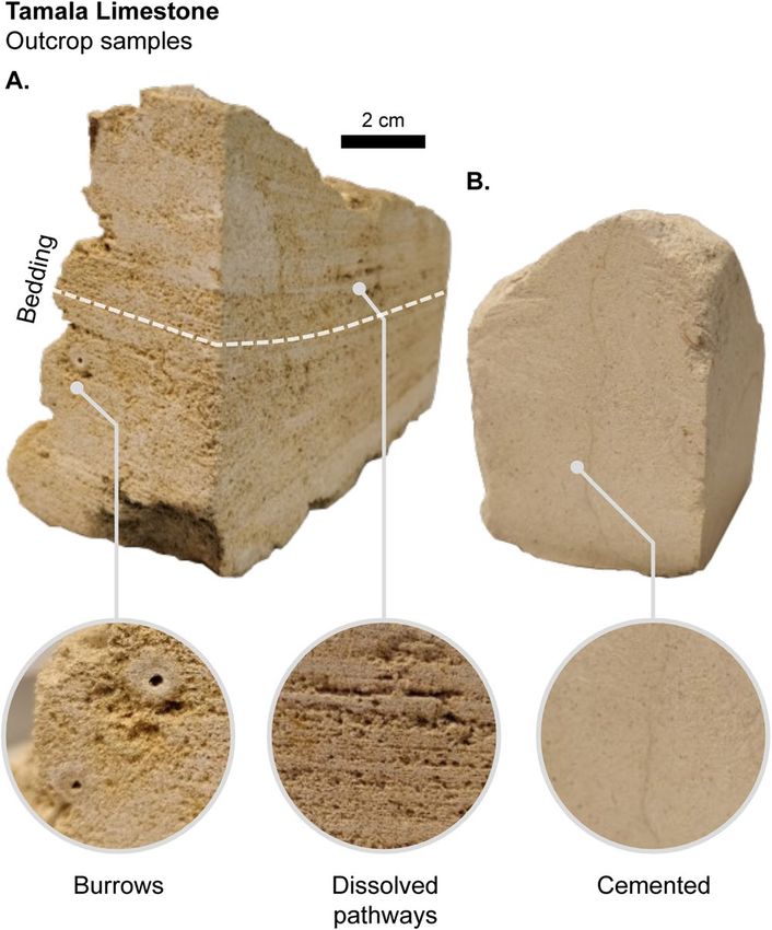
www.nature.com/scientificreports/                                                              www.nature.com/scientificreports

                           Figure 1. Schematic of a shallow coastal groundwater water system in an urban setting and our research
                           outline. The multidisciplinary research is partitioned into six connected parts spanning geology, method of
                           acquisition and processing of well data, numerical groundwater modelling and geophysical methods. An
                           example of the type of questions addressed in each part is provided.

                           terrestrial groundwater flowing toward the ocean and the landward extent of the seawater wedge for high-quality
                           aquifers.
                               Any reduction in fresh groundwater flowing towards the ocean can potentially cause seawater intrusion. This
                           impacts private bores, irrigation systems, and access to potable water1–3. It can also affect sensitive near-shore
                           ecosystems that rely on the nutrients supplied from terrestrial submarine groundwater discharge4–7. This can alter
                           groundwater chemistry with significant environmental and economic consequences8–12. Research into monitor-
                           ing coastal groundwater systems and the seawater wedge provides inputs to managing and maintaining healthy
                           coastal aquifers and ecosystems.
                               Current monitoring practices rely on wells for information on groundwater levels, chemistry, provenance, and
                           age. These data are needed to build numerical groundwater models suitable to predict the consequences of water
                           resource decisions. Drilling and wireline logging are typically used to infer lithology and hydraulic properties.
                           However, this information tends to be localised and can have a dependence on the design of the well or wellfield13.
                               This research systematically traverses the challenges and opportunities faced in monitoring the seawater inter-
                           face in a complex coastal setting. It combines elements from hydrogeology, well-based monitoring technolo-
                           gies, analytical seawater interface solutions, solute transport modelling of increasing complexity, and geophysical
                           methods.
                               The overview shown in Fig. 1 assists the reader in navigating our research, and includes a schematic showing
                           the geometric relationship between groundwater wells and the seawater interface in an urban setting. An example
                           of the type of questions addressed within each part is also provided in Fig. 1. Each part of our research is sum-
                           marized below.

                           •   Part 1: Here we introduce the elements of a coastal karstic aquifer system and our seawater intrusion reference
                               site before comparing it to the hydrogeology of karstic aquifers found worldwide. We include examples of
                               limestone sourced from the reference site and illustrate heterogeneity and dip of the shallow geology using
                               ground penetrating radar.
                           •   Part 2: In this part we identify the influences that may impact the seawater interface at the reference site. The
                               site has experienced significant changes in the position of the seawater interface and groundwater hydraulics
                               throughout the monitoring period. This important site motivates our research concerning methods for char-
                               acterising groundwater throughflow and the seawater interface along shallow coastal aquifer systems.
                           •   Part 3: Part 3 presents the data from the reference site and systematically explores the potential for error in
                               predicting seawater intrusion from groundwater flow using conventional monitoring techniques. Examples
                               from our reference site lead us more sophisticated numerical modelling.

Scientific Reports |   (2020) 10:9866 | https://doi.org/10.1038/s41598-020-66516-6                                                            2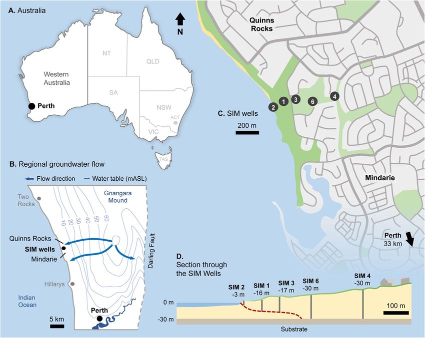
www.nature.com/scientificreports/                                                             www.nature.com/scientificreports

                           Figure 2. Schematic of coastal hydrogeology indicating processes and nomenclature for the seawater interface
                           in a mixed siliciclastic and carbonate near-shore aquifer system. The permeability distribution, groundwater
                           throughflow, and density-driven flow combine to determine the geometry of the seawater/freshwater mixing
                           zone, patterns of groundwater flow within the seawater recirculation cell, and the distribution of submarine
                           discharge. Temporal cycles, such as the seasonal rainfall, pumping from shallow wells, and tidal forcing drive
                           constant groundwater movement in the coastal aquifers. ‘Groundwater throughflow’ describes the volume of
                           groundwater entering the system and flowing towards the coast.

                           •   Part 4: Here we simulate the impacts of anisotropy and heterogeneity on a coastal aquifer. We investigate the
                               impact of dipping hydraulic conductivity anisotropy on the relationship between the landward position of
                               the seawater interface toe and the rate of groundwater flow towards the ocean. Our numerical experiments
                               extend to complex, extremely heterogeneous hydrogeology as found at our seawater intrusion reference site.
                           •   Part 5: This part explores the ability of geophysical techniques to accurately image the seawater interface and
                               coastal hydrogeology. Electrical resistivity imaging (ERI) has the potential to estimate the distribution of
                               salinity in time and space. However, imaging outcomes from ERI can be over-interpreted and we consider
                               the implementation and practicality of ERI for recovering the seawater interface for karstic systems and the
                               reference site.
                           •   Part 6: In Part 6 we focus on the dramatic changes in groundwater velocity that occur proximal to the seawa-
                               ter interface. These details have implications for both short-term and long-term monitoring strategies and
                               solutions. This leads us toward options for new integrated monitoring systems that are tailored to shallow
                               high-quality coastal aquifers.

                           Part 1. Coastal Hydrogeology and a Reference Site
                           Introduction to the near-shore coastal margin. The near-shore coastal margin has nomenclature to
                           describe the specific depositional environments and groundwater processes14. A schematic of this terminology
                           is shown in Fig. 2, and includes features that are commonly associated with recent (Pleistocene) karstic aquifers
                           such as solution pipes and cave systems15,16. The geometric arrangement and distribution of these post-deposi-
                           tional features may play a significant role in determining the geometry of the seawater interface.
                               At the coastal margin, higher density seawater (~1025 kg/m³) sinks beneath the less dense terrestrial ground-
                           water (~1000 kg/m³) forming a wedge shape17,18. The mixing zone describes the area where these two waters
                           interact and form a solute gradient19. The extent of this zone can be highly variable, ranging from sub-meter
                           scales to multiple kilometres20–22, and is chemically-active, with implications for limestone dissolution and
                           re-cementation23,24.
                               Groundwater throughflow and hydraulic conductivity are often used to predict the inland position of the
                           seawater wedge, referred to as the ‘toe’. Groundwater throughflow describes the volume of water flowing in the
                           terrestrial aquifer system towards the coast25. For our cross-sectional model, volume calculations are based on
                           a boundary with unit length (1 m), such that groundwater throughflow is expressed in units of ML/year/m (e.g.
                           see Part 3).
                               In addition to the zones shown in Fig. 2, there are many temporal changes that influence the position of the
                           seawater interface. These include effects of wave surges, beach geometry, tides, rainfall recharge, and groundwa-
                           ter abstraction. These variables ensure that solute distribution and hydraulic heads along coastal margins are in
                           constant motion. In high-quality karstic aquifers, these temporal challenges are compounded by the variability in
                           hydraulic properties associated with high-permeability caves, low-permeability cemented limestone, and aniso-
                           tropy of hydraulic conductivity.
                               Supplementary Table S1 contains a summary table of spatial and temporal parameters that can affect the posi-
                           tion and geometry of the seawater wedge. We will provide specific examples illustrating the potential impact of
                           heterogeneity and anisotropy of hydraulic conductivity on the seawater wedge in Part 4.

                           An urban reference site where seawater intrusion has occurred. Increase in global population den-
                           sity at coastal margins and associated demand for high-quality, low-cost water can significantly impact coastal

Scientific Reports |   (2020) 10:9866 | https://doi.org/10.1038/s41598-020-66516-6                                                          3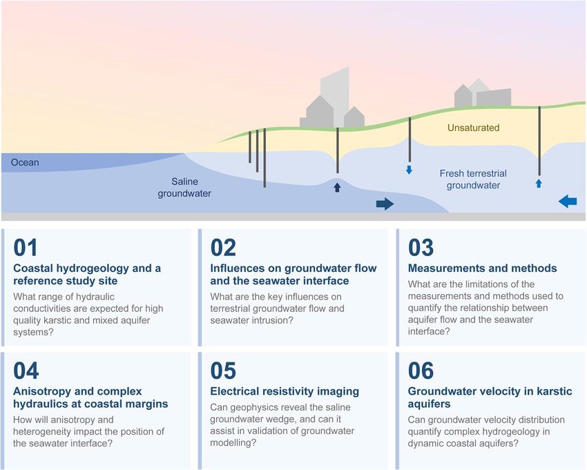
www.nature.com/scientificreports/                                                              www.nature.com/scientificreports

                           Figure 3. Maps providing location and characterisation of the Quinns Rocks seawater intrusion monitoring
                           (SIM) reference site in Perth, Western Australia. (A) The location of Perth relative to Western Australia. (B) The
                           regional groundwater contours, which are approximately parallel to the coastline at Quinns Rocks indicating
                           groundwater flows towards the coast. (C) The location of the SIM wells relative to Quinns Rocks, which have
                           been monitored since 1990. (D) A cross-section of the SIM wells, including the impermeable clayey substrate
                           and an estimate of the current position of the seawater wedge.

                                                                                                        Mean
                                                               Distance     Ground    Screen Depth (m   Screen
                            Well     Easting     Northing      from         Level     BGL)              Depth
                                                               Shoreline
                            ID       mE          mN            (m)          (m AHD)   From     To       (m AHD)
                            SIM 2    376567.43   6494093.94    30           6.13      7.85     8.85     −2.22
                            SIM 1    376635.39   6494122.71    105          11.04     26.1     27.1     −15.56
                            SIM 3    376719.26   6494142.05    190          15.18     31.87    32.87    −17.19
                            SIM 6    376900.26   6494133.29    360          24.03     53.58    54.58    −30.05
                            SIM 4    377084.02   6494174.60    550          31.34     60.43    61.43    −29.59

                           Table 1. Details of the SIM wells including approximate distance from shoreline and depth of the screens below
                           ground level (m BGL).

                           aquifer systems. Our research site in Quinns Rocks, approximately 35 km north of Perth, Western Australia, has
                           experienced a rapid increase in population and urban development during the period of monitoring. Perth, the
                           capital of Western Australia, is one of the lowest population density cities worldwide (~323 persons per square
                           kilometre26,27). However the majority of urban sprawl is occurring along the coastal margins28.
                               The location of the seawater intrusion monitoring (SIM) wells at Quinns Rocks is shown in Fig. 3. It includes
                           the minimum regional groundwater level contours in the upper superficial aquifer for May 200329. It also includes
                           a cross-section through the SIM wells and the approximate position of the seawater interface in 2018. Regional
                           groundwater flow is perpendicular towards the shoreline30. The shallow hydraulic gradients of the regional water
                           level contours approaching the shoreline suggest high permeability in the mixed limestone aquifers typical of
                           Perth’s coastal margin31,32. The details of the SIM well completions are found in Table 1, including the location and
                           depth of the screened intervals.

                           The shallow geology and hydraulics at coastal margins.             A fundamental step in creating a valid and
                           practical groundwater model is to analyse local hydrogeology. Groundwater management often relies on predic-
                           tive groundwater modelling to determine the future impact of groundwater allocations and water supply options.
                           In karstic groundwater systems, aquifer hydraulics can be highly variable over short distances33–35. Localised
                           high-permeability conduits coupled with extremely low-permeability layers of cemented limestone can form

Scientific Reports |   (2020) 10:9866 | https://doi.org/10.1038/s41598-020-66516-6                                                            4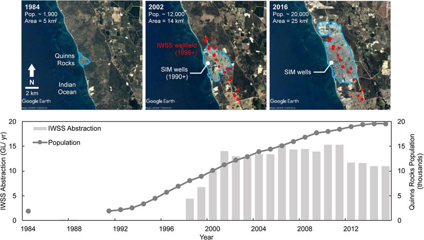
www.nature.com/scientificreports/ www.nature.com/scientificreports
Figure 4. Ranges of hydraulic conductivity estimated at sites along the coastal margin of Perth (shown in
purple) and other karstic environments around the world (shown in yellow). Most of the hydraulic conductivity
in the Perth region fall within the mid-to-upper estimate of typical carbonate values (shown in blue). The karstic
aquifers in Perth is known to contain caves and other high-permeability flow pathways that contribute to the
high hydraulic conductivity.
strongly anisotropic aquifer systems34,36. These environments can influence the shape of the seawater interface
and be associated with unconventional seawater wedge geometries21,37–39.
The range of estimated values for hydraulic conductivity found in literature examples from around the world
are compared with examples from the coastal margin of Perth in Fig. 422,32,35,40–50. The hydraulic conductivity of
karstic aquifers can be orders of magnitude higher than clastic aquifers51,52. The hydraulic conductivity along
Perth’s coastal margin is estimated to be between 10 to 10000 m/day, and the estimated average at the Quinns
Rocks reference site is between 130–200 m/day53. Further detail on the estimates local to Quinns Rocks can be
found in Supplementary Tables S2, S3 and S4.
In Perth, the shallow aquifer is dominantly comprised of the Pleistocene-Holocene-aged Tamala Limestone.
The Tamala Limestone is characterised by shallow horizontal cave systems, a lack of directed conduits, cave clus-
tering near the coast, and extensive collapse-dominated cave systems16,54,55. Evidence for these systems is found
in outcrops, accessible cave systems, limestone quarries, and high-resolution ground penetrating radar. These
features introduce a range of challenges in hydraulic modelling, particularly for numerical groundwater model
calibration31,42,56.
Photographic examples of geological fabrics common in the Tamala Limestone are shown in Fig. 5. The sam-
ple labelled Fig. 5B is typical of a well-cemented limestone, and the sample labelled Fig. 5A is a typical of a highly
porous, high-permeability example of Tamala Limestone. This permeable sample (Fig. 5A) shows preferential
dissolution along bedding, which can form extremely high hydraulic conductivity networks throughout some
layers of the aquifer. In contrast, the sample shown in Fig. 5B is fine grained, well cemented, and likely to have
significantly lower hydraulic conductivity.
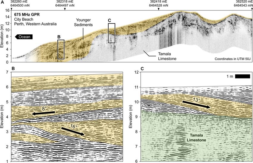
Geological facies at the coastal margin can vary within tens of metres of the coastline. For example, Fig. 6 pre-
sents a high-resolution 675 MHz ground penetrating radar (GPR) profile from City Beach, 10 km west of Perth
CBD. Similar images have been obtained at many locations along Perth’s coastal margin57–60. The GPR data reveals
shallow dipping layers of modern beach and dune facies nested between limestone ridges. The dip of layers in the
beach facies are estimated to be up to 16 degrees. Figure 6A shows an example of layers dipping towards the ocean
(i.e. ~8° west), while Fig. 6B shows layers oriented away from the ocean (dips between 13–16° east). Processing
steps and parameters for the GPR data can be found in Supplementary Table S5.
Two important conclusions stem from the analysis of the karstic near shore setting of the Perth region. These are:
(i) extreme changes in lithological character and associated hydraulic parameters are common, especially perpen-
dicular to the shoreline, and (ii) geological layering is common and likely associated with anisotropy of hydraulic
conductivity throughout Perth’s coastal margin. The influences of anisotropy and complex hydraulic conductivity
distributions are analysed using numerical solute transport modelling later in this research (i.e. Part 4).
Part 2. What drives the relationship between groundwater throughflow and
Seawater Intrusion?
Three influences commonly linked with seawater intrusion include greater net groundwater use (e.g. from
abstraction wells), changes in net vertical flux entering the groundwater system (e.g. rainfall recharge, storm
water infiltrations etc.), and sea-level rise20,61–65. Data was acquired at the Quinns Rocks reference site during a
30-year period, where all three of these factors may have contributed to fundamental changes in the geometry of
the seawater interface.
Scientific Reports | (2020) 10:9866 | https://doi.org/10.1038/s41598-020-66516-6 5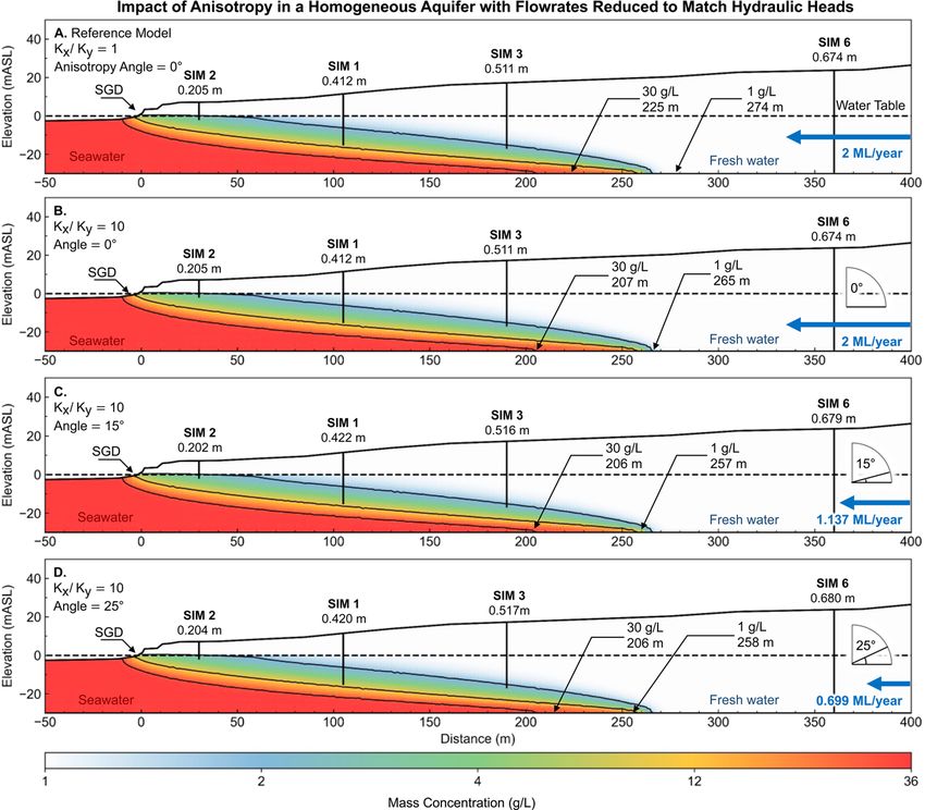
www.nature.com/scientificreports/                                                              www.nature.com/scientificreports

                           Figure 5. Photographs showing samples of the Tamala Limestone with different sedimentary fabrics. (A) A
                           vuggy sample with burrows and dissolved pathways, expected to be highly permeable. (B) A cemented massive
                           fine-grained limestone sample, expected to have considerably lower permeability. This figure highlights the
                           contrast in geological fabrics that directly impact hydraulic conductivity. Large-scale karsts (i.e. caves and other
                           conduits) exist throughout the coastal margin of Western Australia.

                           Figure 6. A ground penetrating radar (GPR) section at Perth’s coastal margins that expresses the typical beach
                           and dune facies and limestone ridges. Panel A shows the GPR energy envelope attribute that highlights the
                           unconformity between the Tamala Limestone and beach/dune facies above. Panel B is a GPR section showing
                           the reflections from sedimentary layering present in the younger facies, with a prevailing dip towards the ocean.
                           Panel C is a GPR section showing the reflections from sedimentary layers dipping approximately 13° landwards
                           (away from the coast) and terminating at an unconformity. This data was collected at the suburb of City Beach,
                           south of Quinns Rocks, using a 675 MHz antenna. Similar examples of dipping beds and limestone ridges occur
                           throughout the coastal margin of Perth15,57,58,187.

Scientific Reports |   (2020) 10:9866 | https://doi.org/10.1038/s41598-020-66516-6                                                            6
www.nature.com/scientificreports/                                                              www.nature.com/scientificreports

                           Figure 7. Set of satellite images showing the rapid expansion of the Quinns Rocks suburb, taken in 1984 (top
                           left), 2002 (top middle) and 2016 (top right), and groundwater abstraction from the IWSS bore field from 1984
                           to 2016 (bottom). The middle satellite image contains the location of the shallow regional wellfield, developed
                           in 1998 for the Integrated Water Supply Scheme (IWSS), and the location of the seawater intrusion monitoring
                           (SIM) wells. The approximate annual groundwater abstraction from the local wellfield during peak production
                           in 2002 was approximately 14 GL/year. The increase in groundwater abstraction during the monitoring period
                           is one potential cause for seawater intrusion at the reference site. Map imagery ©2019 Google Earth, Maxar
                           Technologies.

                              We consider each of these factors with reference to available data for the Quinns Rocks reference site. Our
                           suspicion is that, although the dataset is extensive and spans several decades and wells, isolating any one of these
                           factors is not possible with the data that was collected. Decoupling the relative contributions of each will likely
                           require new monitoring practices.

                           Rapid urbanisation and increased groundwater abstraction at the coastal margins.
                           Groundwater abstraction leading to reduction in terrestrial groundwater flows is often identified as the primary
                           driver for seawater intrusion66–73. Sustainable groundwater management initiatives, such as augmenting rainfall
                           recharge from urban surfaces, and managed aquifer recharge are being developed to reduce the direct depend-
                           ence on shallow groundwater74–80. Systems of aquifer replenishment such as these, introduce another dimension
                           to groundwater flow and reinforce the need for better groundwater monitoring solutions that are better able to
                           decouple multiple influences.
                               The suburbs surrounding the Quinns Rocks reference site have undergone rapid urbanisation and population
                           growth since 1984. The SIM wells were established to assess the impact of development and expansion of Perth’s
                           regional Integrated Water Supply Scheme (IWSS). In total, the IWSS supplies ~289 GL/year to Perth and remote
                           mining towns81. This water is sourced from approximately 43% groundwater, 39% desalinated water, and 18%
                           from surface water82.
                               The recent growth of the Quinns Rocks urban footprint is shown in Fig. 7, and includes population and IWSS
                           groundwater abstraction between 1984 and 2016. The local IWSS wellfield is approximately 2 km to 4 km from
                           the coastline. Shallow groundwater abstraction from the Quinns Rocks region has supplied an average of 12 GL/
                           year since 2003. This forms the majority of coastal groundwater abstraction and accounts for approximately 75%
                           of local groundwater usage42.
                               The development of a groundwater abstraction wellfield parallel to the coast and increase in urban land usage
                           around the reference site is a strong motivation to simulate the local groundwater hydraulics and hydrogeology.
                           Although it may seem easy to attribute the data to groundwater abstraction alone, there are other factors that may
                           have influenced the position of the seawater wedge at this site.

                           Influence of a changing climate and reduced rainfall recharge. The impacts of a rapidly changing
                           modern climate are well-documented83–87. Changes in rainfall patterns and seasonal temperatures will impact
                           groundwater systems88,89. For example, the reduction in winter rainfall can reduce groundwater recharge to a
                           shallow aquifer system, reducing aquifer flows, and ultimately resulting in seawater intrusion90. Bryan, et al64
                           suggest that declining rainfall in the Perth region is the primary cause of seawater intrusion for Rottnest Island,
                           located just 20 km offshore from Perth.
                              Figure 8 shows the cumulative and seasonal (six-monthly) rainfall in Perth between 1944 and 2018. The
                           long-term average rainfall is approximately 700 mm/year. A comparison of the first and last 20-years of the data
                           suggests that the average rainfall has decreased from approximately 834 mm/year (1944 to 1964), to 673 mm/year
                           (1998 to 2018).

Scientific Reports |   (2020) 10:9866 | https://doi.org/10.1038/s41598-020-66516-6                                                           7
www.nature.com/scientificreports/                                                               www.nature.com/scientificreports

                           Figure 8. Graphs showing long-term trends in winter and summer rainfall in Perth, Western Australia. Panel
                           A shows the cumulative rainfall from 1944 to 2018. The average rainfall over the entire period is approximately
                           700 mm/year. Analysis of 20-year trends indicate that an approximately 25% reduction in rainfall has occurred
                           since the start of measurement in 1944. The average rainfall from 1944 to 1964 was 834 mm/year, compared to
                           data from 1998 to 2018 with an average rainfall of 673 mm/year. Panel B shows the total seasonal rainfall for
                           summer and winter showing that a clear decrease in winter rainfall. The decreasing winter rainfall is strong
                           motivation for understanding the follow-on effects to the seawater interface.

                               Analysis of summer (October to March) and winter (April to September) rainfall trends suggest a minor
                           increase of 0.03 mm/year in summer rainfall. However, groundwater recharge from summer rainfall is negligi-
                           ble due to high evapotranspiration rates in Perth60,91. Winter rainfall contributes to the vast majority of rainfall
                           recharge. Analysis of rainfall trends from Fig. 8 suggests an approximately 25% reduction over the 20-year period
                           between 1998 and 2018 compared with the 20-year period between 1944 and 1964.

                           Influence of sea level rise.         Changes in the global sea level, and sea level rise in particular, can affect the
                           position of the seawater interface and the near-shore environment61,92–94. Simulations of the impact of sea level
                           rise suggests that relatively small increases in sea level can potentially move the seawater interface landwards by
                           hundreds of metres95,96. This can extend up to kilometres where karstic high-flow conduits are present21,97.
                               Measurements from a tidal monitoring station located approximately 2 km south of the Quinns Rocks refer-
                           ence site suggest the sea level, on average, has risen by 7.63 mm/year. This is shown in Fig. 9. The government esti-
                           mate for sea-level rise, accounting for ENSO meteorological events, is 9.0 mm/year98. Sea level rise accounts for
                           between 22.8 cm and 27 cm of increased seawater head at the coast over the 30 years of monitoring. The increase
                           in mean sea level is a possible reason behind the observations at the reference site.

                           Part 3. Predicting the Shape of the Seawater Interface: The Value and Limitations of
                           Historical Monitoring Data
                           Monitoring wells provide data required to inform aquifer management. The quality and value of the information
                           gathered is highly dependent on the design and placement of the monitoring well. The demand for the precise
                           management of aquifer systems that works in conjunction with modern numerical groundwater modelling is
                           outpacing both the data type and quality collected from existing monitoring networks.
                               Water level measurements in the seawater intrusion monitoring (SIM) wells at Quinns Rocks between 1990
                           and 2017 are shown in Fig. 10. Panel A shows distribution of measured water levels. The wells SIM 1 and SIM
                           3, nearest to the shoreline, have similar water measurements despite being approximately 80 m apart. The wells
                           SIM 4 and SIM 6 are further inland and have similar measurements despite being over 200 m apart. The shallow
                           hydraulic head gradient between these wells are consistent with a highly permeable aquifer. However, significant
                           differences in hydraulic gradients measured between each pair of SIM wells also suggests a highly heterogeneous
                           distribution of hydraulic parameters.
                               Panel B of Fig. 10 shows the variation in rainfall associated with the typical dry summer and wet winter cycles.
                           The measured water levels are driven by seasonal rainfall cycles. In 1994, the water levels measured in SIM 2,
                           approximately 30 m from the shoreline, vary between 0.00 mAHD (Australian height datum) during the sum-
                           mer months, up to 0.42 mAHD in the winter months. Daily tidal effects account for another 0.5-metre variation
                           superimposed on the measured water levels.
                               Although there appears to be a substantial monitoring dataset at the Quinns Rocks reference site, we notice
                           several inadequacies. Two key outcomes from analysis of the data in Fig. 10 are:

                             I. The temporal sampling rates from manual logging are unable to capture the response of the aquifer system

Scientific Reports |   (2020) 10:9866 | https://doi.org/10.1038/s41598-020-66516-6                                                             8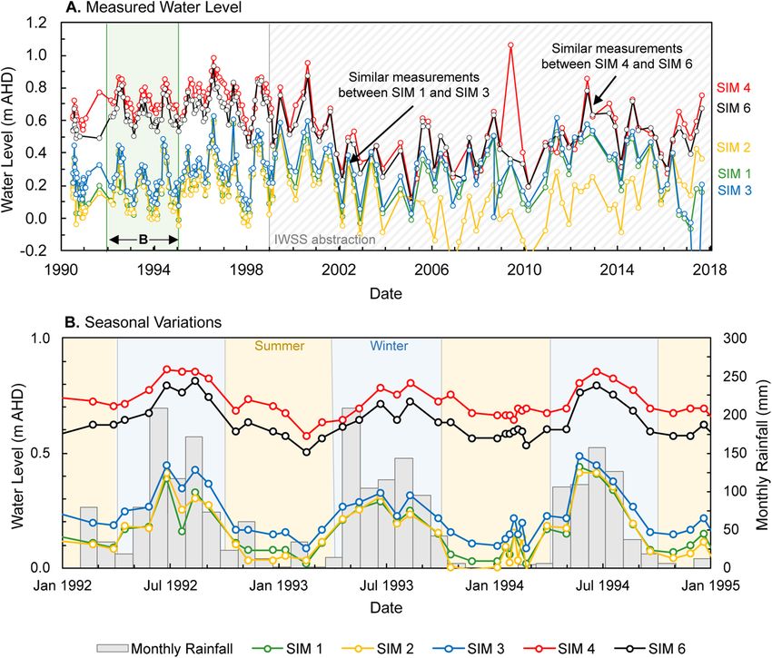
www.nature.com/scientificreports/                                                            www.nature.com/scientificreports

                           Figure 9. Charts showing tidal measurements from a monitoring location near the reference site in meters
                           Australian height datum, mAHD. Panel A shows the raw hourly data since 1992 with a linear fit overlaid. Panel
                           B shows the monthly and yearly averages of the raw data. Tidal levels have risen by approximately 7.63 mm/
                           year since monitoring began. The estimate for sea-level rise that also considers global meteorological events is
                           9.0 mm/year98. The rise in sea level over the monitoring period is a potential factor for landward movement of
                           the seawater interface at the reference site.

                           Figure 10. Set of graphs comparing measured water levels in the seawater intrusion monitoring (SIM) wells
                           to monthly rainfall. Panel A shows measured water levels from 1990 to 2018. The frequency of measurements
                           decreases after the IWSS pumping begins. The measured water levels in SIM 1, SIM 2, and SIM 3, are similar
                           despite separation of 150 m (see Figs. 3 and 7). SIM 4 and SIM 6 also show similar measured water levels
                           despite being separated by close to 200 m. Shallow gradients between these monitoring points suggests zones
                           of localised extreme permeability. Panel B shows water levels and monthly rainfall between 1992 and 1995.
                           Summer periods (October to March) are shaded orange and the winter periods (April to September) are shaded
                           blue. A clear relationship between annual rainfall cycles and water levels is present.

Scientific Reports |   (2020) 10:9866 | https://doi.org/10.1038/s41598-020-66516-6                                                            9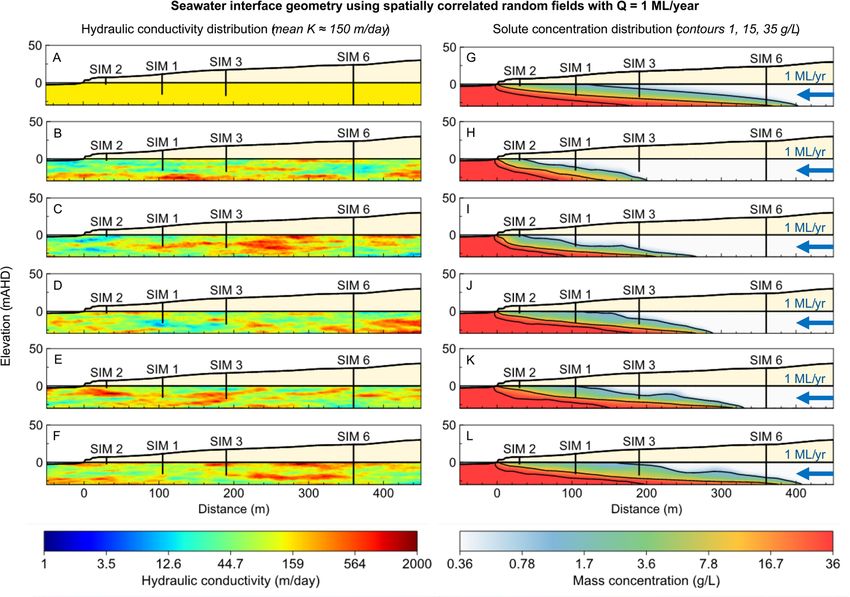
www.nature.com/scientificreports/                                                                     www.nature.com/scientificreports

                           Figure 11. Cross-section through the SIM wells and accompanying time-lapse electrical conductivity (EC) data
                           (1990–2018) showing evidence of seawater intrusion. The current position of the seawater interface is between
                           SIM 3, where EC is equivalent to that of seawater in 2018, and SIM 6, where EC remains that of potable water in
                           2018.

                                from tidal variations, storm surges, and other rapid events (e.g. the spike in SIM 4 in 2009).
                            II. Measuring a single point in depth with conventional PVC wells could mask changes in hydraulic head or
                                solute concentration due to the extreme variability associated with karstic aquifers (e.g. SIM 1, SIM 3 meas-
                                urements and depths).

                           Measurements of water chemistry - What range of seawater interface geometries fit monitor-
                           ing data?. Sampling the properties of the groundwater, such as the electrical conductivity (EC), provides
                           baseline data for identifying seawater intrusion. EC measurements can be approximated to a solute concentration
                           (or total dissolved solids, TDS) using linear approximations99, or by more advanced approximations such as the
                           equation of state of seawater EOS-80100. Details on these calculations as applied at Quinns Rocks are provided in
                           Supplementary Table S6.
                               Over the ~30 years of monitoring, EC data from the SIM wells clearly shows that movement of the seawater
                           interface has occurred (see Fig. 11). The position of the interface in 2018 is somewhere between SIM 3 and SIM 6
                           (i.e. between 180 and 360 m from the shoreline). The solute concentration in SIM 3 is near to that of seawater at
                           ~30 g/L, while in SIM 6 the groundwater has always remained fresh (i.e. potable), with a TDS of 0.3 g/L.
                               A disadvantage of electrical conductivity measurements made in the SIM wells is that the measurements are
                           limited to a single short-screened interval (see Table 1 for the screened intervals in the SIM wells). This allows
                           for many interpretations of the shape of the seawater interface, such as the three hypothetical scenarios that may
                           all correspond to same EC measurements within the SIM wells (see Fig. 12). These scenarios are intended to
                           highlight end members from a range of potential geometries of the seawater wedge over the monitoring period.
                           They include:
                               Scenario 1 (Fig. 12A): Here the toe remains relatively stationary while the seawater interface expands ver-
                           tically. This extreme may occur where there exists an inclined substrate65,101, or an extremely low-permeability
                           lithology exists near the toe95,102.
                               Scenario 2 (Fig. 12B): The seawater wedge expands horizontally. This may occur if horizontal layers have
                           extremely high horizontal hydraulic conductivity, such as directional preference conduit systems21,38,103.
                               Scenario 3 (Fig. 12C): The seawater wedge expands both horizontally and vertically. This is perhaps the most
                           commonly reported movement in seawater intrusion literature2,17,63,104.
                               Long-term groundwater monitoring at the Quinns Rocks reference site shows that movement of the seawater
                           interface has occurred during the monitoring period and that the seawater interface currently exists between
                           200 m and 360 m from the shoreline. However, it is not possible to reconstruct the seawater interface or make
                           conclusions concerning the rate of intrusion from this data alone.

                           Measurements of hydraulics across the wedge transition. Measurement of the hydraulic head at the
                           coastal margin can present greater uncertainty than in other groundwater systems105. These uncertainties can be
                           driven by large variations in groundwater density and a dynamic groundwater environment. A key uncertainty
                           from aquifers containing variable-density groundwater arises when the density of water in the well column is not
                           constant or accurately known when the water level measurement is made.
                               It is often necessary to convert the measured water level in coastal wells to pressure expressed as an equivalent
                           freshwater head for numerical modelling. In a static system, hydraulic head (h i ) is the sum of elevation head (z i )
                           (i.e. the depth of the well screen), and pressure head (h p , i ) (i.e. the length of water column relative to z i )106. This is
                           described by

Scientific Reports |   (2020) 10:9866 | https://doi.org/10.1038/s41598-020-66516-6                                                                     10
www.nature.com/scientificreports/ www.nature.com/scientificreports
Figure 12. Schematic indicating the possible locations of the seawater interface based on measured solute
concentrations from the SIM wells in 1990 (red line) and 2018 (blue line). Panel A shows an example of
primarily vertical movement due to a zone of reduced permeability near to the toe. Panel B shows an example
of horizontal movement of seawater, such as along a high-permeability conduit located near to the base of the
aquifer. Panel C shows an example of both horizontal and vertical movement inland, as would be found in a
homogeneous aquifer.
Pi
hi = z i + hp ,i = z i +
ρig (1)
where h p , i is the hydraulic head from pressure at point i, Pi is the pressure at the well screen, ρi is the fluid density
of the groundwater at the well screen, and g is the acceleration due to gravity.
If unknown variable groundwater density exists, the same hydraulic head (e.g., measured water level) could be
interpreted from different hydraulic pressures. For a system with groundwater of varying density, the ‘equivalent
freshwater head’106,107 represents the column of fresh groundwater required to balance the hydraulic pressure at a
particular depth and groundwater density. The equivalent freshwater head for groundwater at point I with density
ρi is:
ρi ρi − ρf
hf ,i = hi − zi
ρf ρf (2)
where ρf is the density of fresh groundwater.
The range of densities for groundwater proximal to the seawater wedge can lead to multiple interpretations of
hydraulic head. These are illustrated in Fig. 13.
1. If the well is fully screened across the aquifer, the measured water level is equal to the ‘in situ’ hydraulic
head, as shown in Fig. 13A. However, fully-screened wells (Fig. 13, Well A) are susceptible to passive
redistribution of groundwater along the screened interval between layers with different hydraulic proper-
ties108. Any vertical movement or redistribution of seawater via the well-column can affect the groundwater
salinity measurements with consequence for interpretation and monitoring.
2. For the equivalent freshwater head (Fig. 13, Well B), the pressure at the screens is represented by the equiv-
alent column of fresh water. The equivalent freshwater head is always higher than the measured water level
when high-density groundwater is present.
3. The point-water head (Fig. 13, Well C) assumes that the groundwater density at the screened interval exists
throughout the well column. If there is seawater at the screened interval, the measured water level inside of
the well is lower than the true water level outside of the well. This could occur if the screened interval of a
monitoring well is located within the seawater wedge and has been sampled through pumping.
4. The environmental head is calculated assuming that the water within the well is stagnant, and the density
of water inside the well column is equal to the average of water outside of the well106,109 (see Fig. 13, Well
D).
Scientific Reports | (2020) 10:9866 | https://doi.org/10.1038/s41598-020-66516-6 11www.nature.com/scientificreports/ www.nature.com/scientificreports
Figure 13. Schematic representation of uncertainty in the measurement of the hydraulic head from a well
where large changes in solute concentration exist, such as at the seawater interface. The water level measured
in a monitoring well is dependent on the density of water in the well column106,107. Well A is a fully screened
well where the groundwater inside the well column matches that outside of the well. Here the measured water
level is equivalent to the water table. Well B is screened below the water table. If fresh water occupies the entire
water column, the measured water level will be above the water table. Well C shows that if the well column is
filled with seawater, the measured water level will be below the water table. Well D assumes that the density of
the water column is a mixture of fresh and saline waters. This observation is critical to compare measured water
levels with numerical modelling outcomes, which are typically provided as pressure in equivalent freshwater
head. If the water density in the well column is not measured at the time of the water level measurement, there is
significant uncertainty in the equivalent hydraulic head calculation.
A consequence of the above is that the measured water level may not be a reliable input for computation of
groundwater flow conditions in variable density environments. Here specific measurements are required to char-
acterise these groundwater flow systems. We discuss suitable monitoring techniques in the conclusion.
The density of water residing in the well column is often not measured directly, and so must be assumed
from the EC of water samples. This is the situation for the SIM wells at the Quinns Rocks reference site in Perth,
Western Australia. Figure 14 provides an example from the reference site showing the difference in hydraulic
head after computing the equivalent freshwater head (EFH) using the EC-derived mass density100, compared to
the measured water level (MWL). The three dates shown cover the time before seawater intrusion (Fig. 14A),
during active seawater intrusion (Fig. 14B) and a recent date where the EFH gradient is approximately seaward
(Fig. 14C).
The well-to-well hydraulic gradients computed from the measured water levels (i.e. the blue line) in every date
shown in Fig. 14 suggests that groundwater is flowing towards the ocean. In 1992 (Fig. 14A), all of the SIM wells
contain relatively fresh groundwater and the equivalent freshwater head is similar to the MWL. However, by 2011
(Fig. 14B) seawater had progressed beyond the screened interval in SIM 1 and SIM 3 (see Fig. 11). The equivalent
freshwater head suggests a landward hydraulic gradient between SIM 3 and SIM 6.
At first this may seem impossible or at least counterintuitive, however the water level measurements at SIM
1 and SIM 3 must be considered in the context of a seawater recirculation cell (see Fig. 2 and Part 6) that has
potentially moved inland beyond the wells. This presents the possibility of landward flow, albeit at exceedingly
low velocity, in SIM1 and SIM 3 compared with expected groundwater flow towards the ocean past the screen in
SIM 6, which remains fresh.
Estimation of groundwater throughflow from hydraulic gradients. Hydraulic gradients at coastal
margins can be influenced by seasonal changes in groundwater recharge, sea-level variations, and groundwater
abstraction (see sections above). Estimates of throughflow based on hydraulic gradients must also be affected
by how gradients are computed. For example, the gradients are dependent on how aquifer pressure is calculated
(i.e. freshwater head), and localised impacts on aquifer pressure, (e.g. tidal forces and groundwater abstraction).
We estimate groundwater throughflow to the ocean based on hydraulic gradients. The question being
addressed is “Can these methods provide reasonable estimates of groundwater throughflow for calculation of the
landward extent of the seawater interface in a high-quality coastal aquifer system, such as at the Quinns Rocks
reference site”?
There are several assumptions made when estimating groundwater throughflow using the flow-nets and
hydraulic gradients. A typical flow-net analysis assumes that a homogeneous, saturated, and isotropic aquifer
with known boundaries exists110. Extensions to these assumptions exist for anisotropic aquifers111 and partially
saturated flow systems112. The groundwater throughflow, Q, is typically estimated from42
Scientific Reports | (2020) 10:9866 | https://doi.org/10.1038/s41598-020-66516-6 12www.nature.com/scientificreports/ www.nature.com/scientificreports
Figure 14. Charts and schematic showing the equivalent freshwater head compared to the measured water
levels. Here the equivalent freshwater head (EFH) is calculated assuming that the water density around the well-
screen exists throughout the column. Panel A shows a measurement from 1992, which indicates that fresh water
is present. Here the hydraulic gradient is towards the ocean. Panel B shows a measurement from 2011, where EC
measurements at the well-screens suggest that high density seawater is present. Panel C shows a measurement
from 2017, where the EFH in SIM 6 is higher than in SIM 3, suggesting no landward movement of the seawater
interface is occurring. The measured water levels in Panel B suggest a seaward hydraulic gradient, however
the density of water in the well columns has not been considered. Estimation of the EFH with the assumption
that seawater has filled the well column for SIM 1 and SIM 3 in 2011 and 2017 presents significant changes in
groundwater hydraulics in this shallow coastal aquifer system.
Q = TiL (3)
where T is the transmissivity (m²/day), i is the hydraulic gradient across the aquifer (m/m), and L is the width of
the flow-cell (m). Here we assume the flow-cell is of unit length. Transmissivity (T) is the product of the hydraulic
conductivity (K) (m/day) and the thickness of the freshwater saturated aquifer (i.e., where the fresh groundwater
enters the system and occupies the aquifer thickness) (m). For the Quinns Rocks reference site, Kretschmer and
Degens42 estimate the mean hydraulic conductivity to be 130–200 m/day, and the saturated thickness of the aqui-
fer (i.e. depth to confining substrate) to be 30 m42.
Two sets of estimates for the groundwater throughflow (Q) calculated from the hydraulic gradients of the
measured water levels across the SIM wells are shown in Fig. 15. This includes estimates for 1994, prior to regional
groundwater abstraction, and in 2014 after seawater intrusion has occurred. The average groundwater through-
flow is estimated to be 3 ML/year and 1 ML/year respectively. However, it is important to acknowledge the signif-
icant uncertainties that exist in the inputs to these equations, such as the impact of variable density groundwater
on the hydraulic gradient, and the role of heterogeneous hydrogeology on transmissivity.
If EC measurements (and thus some estimate of density) are not made simultaneously with the measurement
of water level, there may be no indication whether the measurement of hydraulic head (and thus the flow from
hydraulic gradient) is affected by the impassable seawater wedge. It may seem appropriate to estimate the gradient
from measurements in wells that are known to be fresh throughout the entire thickness of the aquifer, such as SIM
4 and SIM 6. As shown in Fig. 15, the hydraulic gradients between these two wells are significantly different to the
hydraulic gradient taken across all five SIM wells and yield a far lower estimate of groundwater throughflow (see
Supplementary Figures S1 and S2).
The hydraulic gradients between each of the SIM wells also questions the assumption of homogeneity for the
transmissivity estimate. The steep gradient between SIM 3 and SIM 6 suggests a zone of lower hydraulic conduc-
tivity between the screened intervals of these wells. Shallower inter-well gradients, such as between SIM 1, SIM
2 and SIM 3, can be indicative of high hydraulic conductivity zones. Variable hydraulic gradients across the SIM
wells provides evidence that the aquifer is heterogeneous.
At best, these methods provide a first-order approximation of groundwater flow. Groundwater flow has
reduced from 1994 to 2014, however, the precise value of the groundwater throughflow is uncertain. We will see
that combination of water level measurements and the simple methods described above cannot provide certainty
for the landward extent of the seawater interface or groundwater throughflow.
The seawater interface according to an analytical solution. Analytical solutions, such as those of
Bear and Dagan113, Glover18, Strack114, and others115, estimate the position of the seawater interface based on
averaged measures of hydraulics (e.g. the groundwater throughflow and average hydraulic conductivity). These
solutions tend to simplify the transition between saline and fresh water to a sharp boundary, neglecting the effect
of solute transport phenomena such as dispersion. They can have value in regional scale seawater intrusion stud-
ies where numerical modelling may not be practical71.
Scientific Reports | (2020) 10:9866 | https://doi.org/10.1038/s41598-020-66516-6 13www.nature.com/scientificreports/ www.nature.com/scientificreports
Figure 15. Set of charts showing seasonal variations in groundwater levels, climate and estimated throughflow
at Quinns Rocks. Panel A shows the groundwater throughflow, Q, calculated from hydraulic gradients using
hydraulic conductivity K = 200 m/day. Gradients are computed from the raw measured water levels188. Panel
B shows the mean seasonal temperature and rainfall between 1993 and 2019. Panels C,D show the average
seasonal groundwater levels measured in the SIM wells along with estimated linear fits for 1994 and 2014
respectively. The average groundwater throughflow during 1994 is significantly higher than in 2014, however
we must acknowledge that there are significant uncertainties in the inputs to estimates of hydraulic gradient and
calculation of groundwater throughflow (see also Part 1.3, 3.2, and Fig. 14). At best these methods provide a
first-order approximation of groundwater flow.
The Glover solution is used to illustrate the range of possible seawater toe positions that may be derived using
data at the field site with constraints from groundwater throughflow estimates. The Glover solution is a readily
applied analytical solution that is routinely used to estimate the steady-state toe position of a seawater wedge. It
is expressed as18:
2
2Q Q
z2 = x +
K Δs K Δs (4)
here z is the depth below sea level (e.g. 0 m) to the seawater interface (m), Q is the flow per unit length of the
shoreline (m²/day), K is the hydraulic conductivity of the aquifer (m/day), Δs is the density ratio of seawater to
fresh water, and x is the horizontal distance inland from the shoreline (m).
The range of estimated groundwater throughflow from hydraulic gradient analysis using the average meas-
ured water level across all of the SIM wells is between 3.00 ML/year and 0.48 ML/year. At the lowest estimate of
flow and using a hydraulic conductivity of 200 m/day, the Glover solution places the seawater interface at 1813 m
inland from the shoreline. This estimate is not reasonable for the study site as fresh groundwater is still present
at the SIM 6 monitoring well located only 360 m inland. We suspect that the gross overestimate (1813 m) for the
position of the seawater interface is likely due to the inability of the solution to accommodate hydraulic complex-
ity of the karstic system along Perth’s coastal margins, although there are many uncertainties in the inputs to this
solution as discussed in 3.3.
Scientific Reports | (2020) 10:9866 | https://doi.org/10.1038/s41598-020-66516-6 14www.nature.com/scientificreports/ www.nature.com/scientificreports
Figure 16. Diagram representing the finite element mesh and boundary conditions used for numerical
groundwater flow and solute transport modelling. The mesh is coarse above the saturated zone as no recharge
from the surface is included. Cells surrounding to the water table are included in the aquifer mesh refinement.
The impact of increasing levels of refinement (e.g. number of elements) are provided in Supplementary
Figure S3.
Parameter Value Unit
Hydraulic Conductivity 200 m/day
Seawater Concentration (TDS) 35800 mg/L
Freshwater Concentration (TDS) 358 mg/L
Density Ratio 0.0256 —
Specific Storage 10−4 1/m
Effective Porosity 0.3 —
Molecular Diffusion 10−9 m2/s
Longitudinal Dispersivity 2 m
Transverse Dispersivity 0.2 m
Saturated thickness 30 m
Table 2. Groundwater flow and solute transport modelling parameters used to generate models in FEFLOW.
In the next section, we use numerical solute transport models for a homogeneous aquifer to simulate the posi-
tion of the seawater toe for comparison with the toe position calculated from the analytical solution and estimated
from the field data.
The seawater interface according to a homogeneous numerical transport model-
ling. Numerical groundwater flow and solute transport modelling can replicate phenomena observed at the
seawater interface, such as groundwater mixing and variable density heads. We use FEFLOW 7.2104 to simulate
seawater intrusion into a high quality, high permeability coastal aquifer similar to that found at the Quinns Rocks
reference site. We use a 2D cross-sectional model to describe groundwater throughflow to the ocean using units
of ML/year for a unit thickness (1 m). That is, for an aquifer that is 30 m thick, the groundwater throughflow is the
rate that water passes through a surface with dimensions 1 m × 30 m.
The quadrilateral mesh discretisation and boundary conditions used for the finite element model are shown
in Fig. 16. Seawater enters the model through the left boundary and along the top boundary until the coastline
(x ≤ 0 m). The density dependent hydraulic head condition ensures that seawater drives inland116. The flow of
fresh groundwater (TDS ~358 mg/L) into the model is controlled by a fixed flux condition along the boundary at
the right for z ≤ 0 m. The substrate at the base of the model (z = −30 m) represents a no-flow boundary.
Table 2 summarises the material parameters used in the groundwater flow and solute transport model.
Simulations were run until no further changes to the position of the seawater toe were observed. The minimum
mass concentration values are described in Part 1, while the maximum mass concentration is estimated from the
sea-surface salinity local to Perth117. The density ratio is set to 0.0256 after Fofonoff and Millard Jr118. The disper-
sivity is estimated based on Smith, et al.31, Narayan, et al.119.
We simulate the systematic reduction of groundwater throughflow and show the change in solute distribution
in Fig. 17. The groundwater throughflow is reduced from 4 ML/year to 1 ML/year and covers the range of ground-
water throughflow estimated for the Quinns Rocks reference site. The groundwater throughflow is not reduced
again once the SIM wells furthest inland become salinised. Figure 17C–F shows that halving the groundwater
throughflow will double the inland position of the toe for the homogeneous aquifer.
A comparison of the simulated data with measured field data from 1994 and 2014 (Fig. 17A,B) shows that
no throughflow rate can be combined with a homogeneous aquifer to achieve a suitable match. The EC in SIM 6
is the strongest constraint for the inland position of the seawater wedge, which, as of 2019 remains that of fresh
water. To satisfy the solute concentration condition at SIM 6 with this homogeneous aquifer model, ground-
water throughflow must remain above 2 ML/year, which results in the simulated hydraulic head being signifi-
cantly higher than any of the measured values. This numerical experiment also highlights the counterintuitive
shape of the simulated hydraulic gradients. As denser seawater passes the monitoring well screen, the equivalent
Scientific Reports | (2020) 10:9866 | https://doi.org/10.1038/s41598-020-66516-6 15www.nature.com/scientificreports/ www.nature.com/scientificreports
Figure 17. Set of images showing the simulated seawater interfaces for a range of groundwater throughflow
in a 30 m thick aquifer with hydraulic conductivity 200 m/day over an impermeable substrate (i.e., average
values for the Quinns Rocks reference site). Charts A and B show the measured water levels (MWL) and
equivalent freshwater head (EFH) in 1994 and 2014. The EFH is calculated assuming that the groundwater
at the well screen occupies the entire well column. Images C, D, E and F show the solute concentration
distribution corresponding to groundwater throughflow of 4, 3, 2, and 1 ML/year respectively. According to
this homogeneous aquifer model, groundwater throughflow must remain above 2 ML/year at Quinns Rocks
to maintain fresh groundwater at SIM 6; however, this results in significantly greater simulated hydraulic head
than the field observations. We find that there is no combination of hydraulic conductivity and throughflow
for a homogeneous aquifer that can reasonably explain both measured values of hydraulic head and solute
concentration at the reference site. This points towards high contrast in hydraulic parameters within the aquifer
as a strong influence on the landward extent of saline groundwater.
freshwater head can rise above the hydraulic head for wells further inland (in fresher water). This is shown by the
hydraulic gradient between SIM 6 and SIM 4 (Fig. 17A,B).
Comparison of numerical and analytic solutions for the landward extent of seawater. The
landward extent of the seawater interface is fundamental information required coastal groundwater resource
management. Although the analytical solution can provide a quick answer, we suspect that in practice it may also
lead to significant error.
In Fig. 18, we compare the landward extent of the seawater toe using the analytical Glover solution with
numerical simulations (see Table 2). Numerical modelling with throughflow of 1 ML/year places the toe at 434 m
inland (i.e. this is the landward extent of the 34 g/L contour). For the same groundwater throughflow, the Glover
solution places the toe at 875 m inland. This is almost twice as far inland as compared to the numerical model (see
Fig. 17F). For a homogeneous aquifer, there is a significant difference between analytical and numerical solutions.
If we accept the simplifying assumption of a homogeneous aquifer for the Quinns Rock site, the numerical
solution suggests that the reduction in groundwater throughflow between 1990 and 2018 should result in the sea-
water wedge moving over 500 m inland, to 750 m from the shoreline. This cannot be correct, as the groundwater
in SIM 6, ~360 m from the ocean, has always remained fresh. This supports the case that neither the analytical
Scientific Reports | (2020) 10:9866 | https://doi.org/10.1038/s41598-020-66516-6 16You can also read