Environmental DNA simultaneously informs hydrological and biodiversity characterization of an Alpine catchment
←
→
Page content transcription
If your browser does not render page correctly, please read the page content below
Hydrol. Earth Syst. Sci., 25, 735–753, 2021
https://doi.org/10.5194/hess-25-735-2021
© Author(s) 2021. This work is distributed under
the Creative Commons Attribution 4.0 License.

Environmental DNA simultaneously informs hydrological and
biodiversity characterization of an Alpine catchment
Elvira Mächler1,2 , Anham Salyani3 , Jean-Claude Walser4 , Annegret Larsen3,5 , Bettina Schaefli3,6,7 ,
Florian Altermatt1,2 , and Natalie Ceperley3,6,7
1 Eawag:   Swiss Federal Institute of Aquatic Science and Technology, Department of Aquatic Ecology,
Überlandstrasse 133, 8600 Dübendorf, Switzerland
2 Institute of Evolutionary Biology and Environmental Studies, University of Zurich, Winterthurerstrasse 190,

8057 Zürich, Switzerland
3 Faculty of Geosciences and Environment, Institute of Earth Surface Dynamics, University of Lausanne,

1015 Lausanne, Switzerland
4 Federal Institute of Technology (ETH), Zürich, Genetic Diversity Centre, CHN E 55 Universitätstrasse 16,

8092 Zürich, Switzerland
5 Soil Geography and Landscape Group, Wageningen University, Droevendaalsesteeg 3,

6708 PB Wageningen, the Netherlands
6 Geography Institute, University of Bern, 3012 Bern, Switzerland
7 Oeschger Centre for Climate Change Research, University of Bern, Switzerland

Correspondence: Elvira Mächler (elvira.maechler@gmail.com) and Natalie Ceperley (natalie.ceperley@giub.unibe.ch)

Received: 23 September 2020 – Discussion started: 7 October 2020
Revised: 24 December 2020 – Accepted: 29 December 2020 – Published: 18 February 2021

Abstract. Alpine streams are particularly valuable for down-       conveyed by naturally occurring hydrologic tracers. Between
stream water resources and of high ecological relevance;           March and September 2017, we sampled water at multiple
however, a detailed understanding of water storage and re-         time points at 10 sites distributed over the 13.4 km2 Vallon
lease in such heterogeneous environments is often still lack-      de Nant catchment (Switzerland). The sites corresponded to
ing. Observations of naturally occurring tracers, such as sta-     three different water types and habitats, namely low-flow or
ble isotopes of water or electrical conductivity, are frequently   ephemeral tributaries, groundwater-fed springs, and the main
used to track and explain hydrologic patterns and processes.       channel receiving water from both previous mentioned water
Importantly, some of these hydrologic processes also create        types.
microhabitat variations in Alpine aquatic systems, each in-           Accompanying observations of typical physicochemical
habited by characteristic organismal communities. The inclu-       hydrologic characteristics with eDNA revealed that in the
sion of such ecological diversity in a hydrologic assessment       main channel and in the tributaries, the biological richness
of an Alpine system may improve our understanding of hy-           increases according to the change in streamflow, dq/dt,
drologic flows while also delivering biological information.       whereas, in contrast, the richness in springs increased in cor-
Recently, the application of environmental DNA (eDNA) to           relation with electrical conductivity. At the catchment scale,
assess biological diversity in water and connected habitats        our results suggest that transport of additional, and proba-
has gained popularity in the field of aquatic ecology. A few of    bly terrestrial, DNA into water storage or flow compartments
these studies have started to link aquatic diversity with hydro-   occurs with increasing streamflow. Such processes include
logic processes but hitherto never in an Alpine system. Here,      overbank flow, stream network expansion, and hyporheic ex-
we collected water from an Alpine catchment in Switzerland         change. In general, our results highlight the importance of
and compared the genetic information of eukaryotic organ-          considering the at-site sampling habitat in combination with
isms conveyed by eDNA with the hydrologic information              upstream connected habitats to understand how streams inte-

Published by Copernicus Publications on behalf of the European Geosciences Union.
736                                                                E. Mächler et al.: Environmental DNA in the Vallon de Nant

grate eDNA over a catchment and to interpret spatially dis-           can relatively consistently discriminate snowmelt, rain, and
tributed eDNA samples, both for hydrologic and biodiversity           potentially glacier melt, which all contain few solutes due to
assessments. At the intersection of two disciplines, our study        their little contact with rock and soil surfaces, from ground-
provides complementary knowledge gains and identifies the             water, which typically has much higher levels of solutes due
next steps to be addressed for using eDNA to achieve com-             to extended contact with surfaces (Williams et al., 2006; Coc-
plementary insights into Alpine water sources. Finally, we            hand et al., 2019; Kobierska et al., 2015). On the other hand,
provide recommendations for future observation of eDNA in             water temperature cannot be used as a conservative tracer be-
Alpine stream ecosystems.                                             cause it quickly changes along a water course, but it can pro-
                                                                      vide insights on separating surface water (having a strong
                                                                      diel variation) and influxes of water from the subsurface
                                                                      (having more constant temperatures; Constantz, 1998; Co-
1   Introduction                                                      mola et al., 2015; Hoehn and Cirpka, 2006; Westhoff et al.,
                                                                      2007; Selker et al., 2006). Finally, stable isotopes of water,
Alpine environments are often considered to be water towers           δ 18 O and δ 2 H, have classically been used as tracers of source
for lowland areas (Viviroli et al., 2007) and hotspots for bio-       water, flow paths, and precipitation contributions. Precipita-
diversity (Körner, 2002) and will likely be disproportionately        tion becomes depleted, or has lower values, when it falls at
affected by climate change compared to other areas (Jacob-            higher elevations and in lower temperatures, especially when
sen et al., 2012; Grabherr, 2009). The complex topography             it falls as snow. This natural variation in isotopic ratio in pre-
of mountain areas results in a tremendous variation in the            cipitation according to season and elevation offers clues as
physical environment in terms of elevation, slope, and expo-          to when and where it entered the system. However, in high
sure, which subsequently creates large gradients of received          Alpine contexts, it often falls short in offering additional in-
radiation and thus extreme variations in temperature at small         sights into dominant flow paths because the isotopic ratio of
scales. Subsequently, the topography and temperature gra-             all potential water sources is dominated by the precipitation
dients translate into a landscape with an enhanced hetero-            phase of incoming water (rain versus snow; Lyon et al., 2018;
geneity of potential water flow paths. These paths are addi-          Beria et al., 2018; Penna et al., 2018). Landwehr and Coplen
tionally governed by highly seasonal incoming water (rain or          (2006) improved upon the direct observation of isotopes with
snow), which is released as a seasonal alternation of runoff          the line-conditioned excess (lc-ex), a metric that is equal to
from rain, stored snow, and snowmelt. Consequently, chan-             the residual between two isotopes of water, δ 18 O and δ 2 H.
nel networks in Alpine areas are known to regularly expand            Higher values of lc-ex thus indicate when water has experi-
and contract, leaving a portion of streams ephemeral (Godsey          enced losses to evaporation or other fractionation, allowing
and Kirchner, 2014; van Meerveld et al., 2019).                       it to be used as an additional tracer alongside the ratios of
   Despite the importance of mountain water resources, hy-            oxygen and hydrogen isotopes individually.
drologic processes are still often poorly characterized in                Similar to their high variations in water proprieties, Alpine
mountain catchments. From a hydrologic as well as from an             catchments are typically dominated by high fluctuations in
ecological viewpoint, the central phenomenon determining              discharge and corresponding changes in the extent of the
habitat availability is the origin of stream water, for example,      stream network (Godsey and Kirchner, 2014). The change in
whether streams are fed by seasonal snowmelt or by recent             discharge at a catchment’s outlet over time, dq/dt, can thus
precipitation (Nolin, 2012; Cochand et al., 2019; McGuire             serve as a proxy for stream network recession and expan-
and McDonnell, 2015). In headwaters of mountain environ-              sion (Biswal and Marani, 2010; Mutzner et al., 2013). When
ments, the relevant hydrologic mechanisms are difficult to            dq/dt is negative, it indicates how the upstream stream net-
observe because they occur out of direct reach, for exam-             work contracts and the rate at which stored water, whether
ple in the atmosphere or the subsurface (McDonnell et al.,            in soil or as groundwater, continues to flow into the stream.
2007). There is an ongoing search for hydrologic tracers to           When it is positive, it indicates network expansion after
decompose river water into its most recent storage compart-           a precipitation input event, whether rainfall or snowmelt,
ment (e.g., glacier, snow, soil, groundwater) and to identify         which has led to subsurface saturation, overland flow, and
when and where it entered the stream network (Abbott et al.,          fast subsurface flow.
2016; Blume and Van Meerveld, 2015; Williams et al., 2009;                In the highly variable Alpine environment, water flow and
Mosquera et al., 2018).                                               its properties can mean proliferation or eradication of habi-
   Spatial and temporal variations in the physicochemical             tats; thus it determines persistence of biodiversity. Purely dis-
properties of water in Alpine catchments, such as in temper-          ciplinary views to address current global changes and the
ature, discharge, stable isotopes, and electrical conductivity        consequences for habitats and diversity are not sufficient to
(EC), offer clues to identify water flow from glacier, snow,          address this challenge. Future indicators that simultaneously
soil, and groundwater and its associated timescales (Zuecco           offer information about the hydrological and ecological di-
et al., 2019; Tetzlaff et al., 2015; Penna et al., 2014; Klaus        mensions of the environment may be critical to get a coherent
and McDonnell, 2013; Beria et al., 2018). For example, EC             and complete picture of aquatic systems. Such novel methods

Hydrol. Earth Syst. Sci., 25, 735–753, 2021                                              https://doi.org/10.5194/hess-25-735-2021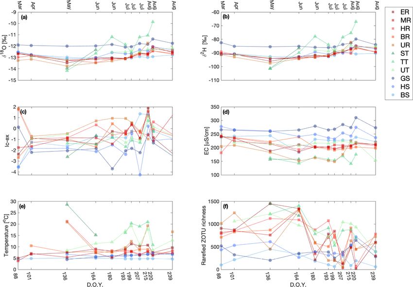
E. Mächler et al.: Environmental DNA in the Vallon de Nant                                                                     737

should complement existing tools by either improving their         et al., 2013), naturally occurring DNA has just started to enter
accuracy or by revealing additional, complementary insights        into the repertoire of hydrologic tracers (Good et al., 2018;
into a system, such as complementing hydrologic informa-           Carraro et al., 2018, 2020a, b). Particularly, it may comple-
tion with biological information. Alpine aquatic systems are       ment existing physical tracers by not only indicating possible
especially suited for such an interdisciplinary approach, be-      water sources, but also indicating their organismal communi-
cause the high variability and complexity of physicochem-          ties, which are regularly used as a water quality component.
ical properties and dynamic flow paths is known to be                 In this study, we tested whether the inclusion of eDNA in
matched by equally complex and diverse biological habitats         a hydrologic assessment of an Alpine system improves our
that are inhabited by highly specialized organismal commu-         understanding of hydrologic flows while simultaneously de-
nities (Brown et al., 2003; Milner and Petts, 1994; Ward,          livering biological information. We also explored how this
1994). For example, midges of the genus Diamesa are char-          would benefit biologists seeking to quantify Alpine diversity
acteristic or sometimes even the only inhabitants of rivers        by providing clear recommendations regarding where and
dominated by glacial input, resisting the cold temperatures        when to sample eDNA in river networks for assessments of
and high turbidity (Milner and Petts, 1994). Contrarily, ple-      diversity. To do so, we repeatedly sampled water in an Alpine
copterans of the genus Protonemoura or the species Leuctra         catchment from spring to summer. We selected 10 sites cor-
nigra are typical inhabitants of Alpine springs (Staudacher        responding to three different water types: low-flow streams
and Füreder, 2007; Hahn, 2000). The same is true for mi-           that are likely ephemeral, fed by snowmelt, glacier melt, or
croorganisms, where higher abundances of α-Proteobacteria          rain (tributaries); groundwater emerging from the subsurface
were found in glacial streams than in other aquatic systems,       (springs); and the higher flow stream fed by the other two
likely reflecting the trophic status (i.e., the primary produc-    (main channel). Throughout this study, we will refer to these
tivity) of the habitat (Battin et al., 2004). Finally, algae of    three water types to encompass the characteristic flows and
the genus Chamaesiphon and the species Hydrurus foetidus           sources of this catchment and their corresponding aquatic
are indicative of glacier-dominated sites (Hieber et al., 2001).   habitats. Firstly, we hypothesized that different Alpine wa-
Consequently, the presence and drift of biological organisms       ter types carry significantly different eDNA signals that can
are expected to be not only of high ecological relevance, but      be used to discriminate between them. Secondly, we hypoth-
also to have the potential to trace connectivity of the stream     esized that hydrologic variability, i.e., the change in stream-
network, a hypothesis which has been confirmed by some             flow and subsurface water flow as observed through various
studies on bacteria (Pfister et al., 2009; Lan et al., 2019) and   physicochemical indicators, drives the temporal and spatial
diatoms (Wang et al., 2017).                                       eDNA signal. Thirdly, we expected the sum of eDNA from
   In recent years, the use of environmental DNA (eDNA)            upstream sampling points to shape the eDNA signal at the
has been shown to be highly powerful for monitoring organ-         most downstream catchment outlet. Our study provides an
isms in aquatic ecosystems (Valentini et al., 2016; Deiner         initial assessment of the spatial and temporal heterogeneity
et al., 2015; Bohmann et al., 2014; Altermatt et al., 2020).       of eDNA in an Alpine stream system. We give concrete rec-
All organisms, ranging from microbes to vertebrates, leave         ommendations for sampling eDNA in this context and iden-
traces of their genetic material in the environment. This DNA      tify opportunities but also challenges to its possible use for
can be collected in environmental samples and is referred          gaining additional hydrologic insights.
to as “environmental DNA” (Ficetola et al., 2008; Taber-
let et al., 2012). With a single sampling technique, eDNA
samples can detect communities of a broad taxonomic scale          2   Methods
by using a high-throughput sequencing approach of a bar-
                                                                   We monitored eDNA in an Alpine catchment in Switzer-
coding region, so-called metabarcoding. In an ideal case,
                                                                   land in parallel with hydrometeorological observations. On
the barcoding region allows for identification at the level of
                                                                   11 field days in 2017 (for exact dates see Table S1 in the Sup-
species. In stream systems, several studies have shown that
                                                                   plement), we sampled eDNA and simultaneously observed
eDNA can travel for distances of tens to hundreds of kilo-
                                                                   the EC, water temperature, and stable isotope ratios of the
meters (e.g., Deiner and Altermatt, 2014; Pont et al., 2018).
                                                                   water (δ 18 O, δ 2 H). In addition, we continuously monitored
Thus, stream networks congregate eDNA from upstream ar-
                                                                   discharge at the catchment outlet and meteorological param-
eas (Deiner et al., 2016), highlighting its potential to derive
                                                                   eters at four stations distributed across the catchment (Fig. 1).
flow path information at the catchment level as well as to
                                                                   We first describe the field site and instrumentation for hydro-
reconstruct diversity patterns using hydrologic models (Car-
                                                                   logic observations. Then, we explain the eDNA sampling and
raro et al., 2020a). Recent work from lowland streams and
                                                                   laboratory procedures before describing the data analysis and
their wastewater inflows also showed that mixing of different
                                                                   statistics used.
water sources can be traced to a high level of reliability with
eDNA (Mansfeldt et al., 2020). While artificially introduced
DNA attached to particles has already been used as a hydro-
logic tracer (Dahlke et al., 2015; McNew et al., 2018; Foppen

https://doi.org/10.5194/hess-25-735-2021                                           Hydrol. Earth Syst. Sci., 25, 735–753, 2021
738 E. Mächler et al.: Environmental DNA in the Vallon de Nant
2.1 Site description
The Avançon is the main stream in the Vallon de Nant catch-
ment (Canton of Vaud, Switzerland; Fig. 1). The 13.4 km2
catchment ranges from 1200 m a.s.l. (as defined by a gaug-
ing station at 46.25301◦ N, 7.10954◦ E) to 3051 m a.s.l. (Le
Muveran). It has a dominant north exposition, with almost
no direct sun during winter in its upper parts, allowing a
small glacier (Glacier de Martinets, 0.36 km2 ; GLAMOS,
1881–2018) to persist at relatively low elevation. Permafrost
is likely present above 2400 m a.s.l. (Giaccone et al., 2019).
The streamflow regime is of the nivo-pluvial type (Aschwan-
den and Weingartner, 1985), with a monthly streamflow
peak in June. The stream network in the catchment consists
of streams that have been classified as first-, second-, and
fourth-order streams according to the Strahler terminology.
Correspondingly they have been characterized as having low
(< 0.05 m3 s−1 and occasionally ephemeral) and medium an-
nual mean discharge (0.05–1 m3 s−1 ), which we will refer to
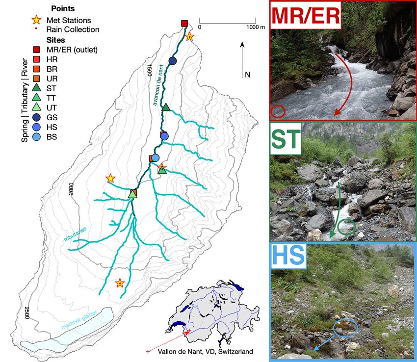
Figure 1. Map of Vallon de Nant showing sampling sites and stream
as tributaries and main channel, respectively; see Schaffner network. Main channel sites are marked by red squares, tributaries
et al. (2013), Pfaundler (2005), and Table S2 in the Supple- by green triangles, and springs by blue circles; in all three cases,
ment. The stream network is fed by melt from the seasonal shading lightens with elevation. The two letter codes are used to
snowpack including avalanche deposits, which can persist identify the sites (see also Table S2). The main channel is the
into the summer months, and by drainage from the soil (abun- Avançon de Nant, which is shown in dark cyan. Predominately
dant unconsolidated alluvium) and from deeper groundwater ephemeral tributaries of various origins are shown in turquoise. The
via springs. Permafrost and glacier melt enters the catchment remaining Glacier de Martinet is shown in light blue. Yellow stars
in the upper tributaries. with a red dot in their center indicate where meteorological stations
also corresponded to points of rain collection for isotope analysis.
Discharge observation occurred at the outlet, which is indicated by
2.2 Hydrologic parameters
the MR/ER sampling site icon. The location of the catchment on an
outline of Switzerland with its main hydrologic network is shown
2.2.1 Instrumentation and field observation to the lower right. On the right are pictures of the main channel
(MR/ER, top), a tributary (ST, middle), and a spring (BS, bottom).
Water level at the outlet (Fig. 1) was measured using a VEG- Colored circles show sampling points, and arrows show direction of
APULS WL-61 optical height gauge (VEGA, Schiltach, Ger- water flow. Elevation and river network data courtesy of the Swiss
many) over a geophone weir, and discharge was determined Federal Office of Topography (geodata © swisstopo (DV084371)).
using an established rating curve (Ceperley et al., 2018). A
network of four distributed meteorological stations (at 1253,
1500, 1780, and 2100 m a.s.l.; Fig. 1) included precipita- mersed at the outlet for the entire year, and logged tempera-
tion and air temperature, mainly measured with a Lufft-WS ture every minute.
300/400 (Fellbach, Germany), and solar radiation, measured At each point, temperature and EC were measured simul-
with an Apogee incoming radiometer (SP230, Logan, Utah, taneously with water sampling using a WTW probe (multi-
USA), mounted in an energetically autonomous wireless net- 3510 with a IDS-tetracon-925, Xylem Analytics, Germany).
work with a GPRS connection (Sensorscope Sarl, Lausanne, When temperature was not measured during sampling, it was
Switzerland; Michelon, 2017; Ingelrest et al., 2010). At a sin- substituted by an observation from the continuous water tem-
gle point (1253 m a.s.l.), a MADD tipping bucket rain gauge perature loggers. When EC was not measured in the field, it
provided back-up measurements (Fallot, 2013, Yverdon, was post-analyzed using a glass 6 mm probe in the laboratory
Switzerland,). Data from the Swiss automatic meteorologi- (Jenway 4510, Staffordshire, UK).
cal station network (MeteoSwiss, 2019) are used to fill gaps A total of 135 composite rain samples were collected using
of the local observations (12 missing days in 2017). Water funnels flowing into insulated bags at three locations corre-
temperature was recorded every 15 min or more frequently at sponding to the rain gauges (1253, 1500, and 2100 m a.s.l.;
all but one sampling site (TT; see Fig. 1) with Hobo temper- see Fig. 1) and emptied approximately weekly or biweekly
ature/light pendants and one temperature/conductivity log- during the summer seasons between June 2016 and Novem-
ger for parts of the study period (Supplement, Table S2; On- ber 2018 (3). In total between February 2016 and April 2018,
set Computer Corporation, Bourne, MA, USA). One WTW- 199 snow samples were collected in a distributed manner
Tetracon 325 (Xylem Analytics, Germany) was installed, im- across the catchment, with between 3 and 26 samples per
Hydrol. Earth Syst. Sci., 25, 735–753, 2021 https://doi.org/10.5194/hess-25-735-2021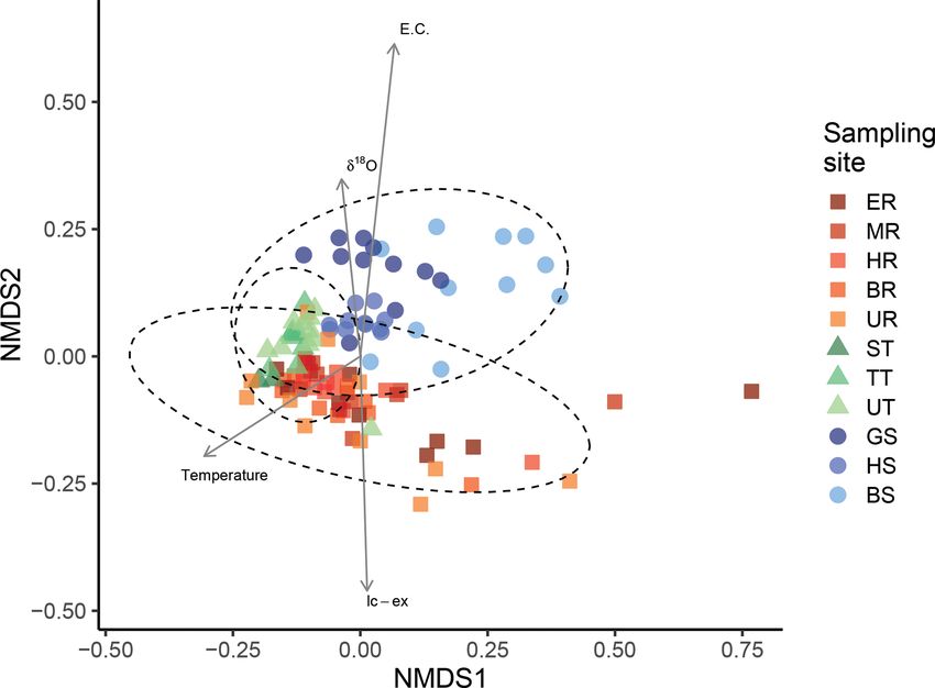
E. Mächler et al.: Environmental DNA in the Vallon de Nant                                                                      739

month in the winter, and included the entire snowpack depth         Energy Agency). Delta units of isotope compositions are re-
when possible (see additional details in Table S3).                 ported (Coplen, 1994).
   The snow-covered area was calculated as a ratio from 0              All available samples of precipitation were used to deter-
to 1 over the non-forested part of the catchment using 21 ,         mine a local meteoric water line (LMWL; Fig. S2), which
images and 24 Sentinel-2 images between August 2016 and             was used to determine the line-conditioned excess (lc-ex, L),
December 2017 (Michelon et al., 2018). Time steps between           or offset from the LMWL:
the images ranged from 0 to 43 d, averaging 11 d. A linear in-
terpolation of the combined time series was used to provide a       L = δ 2 H − 7.82 · δ 18 O − 10.47.                          (1)
fractional area covered with snow per sampling date. Satellite
                                                                    A positive value of lc-ex falls above the LMWL and a nega-
images were taken on average 7 d before or after sampling,
                                                                    tive one below (Landwehr and Coplen, 2006). The value of
though some were on sampling days and others were up to
                                                                    lc-ex reflects a combination of the source water and the phys-
20 d prior or after.
                                                                    ical processes that have occurred since precipitation, with
                                                                    more negative values indicating more evaporation and con-
2.2.2   Flow calculations
                                                                    densation (Sprenger et al., 2016).
Both baseflow and dq/dt were calculated from the discharge          2.3     Environmental DNA
data at the outlet at the highest recorded streamflow reso-
lution (10 min). Baseflow was defined as the lowest value           2.3.1    Sampling and laboratory procedure
in a 10 d moving window. On the other hand, the change
in discharge over time, dq/dt, was determined as the slope          eDNA was sampled by filtering 250 mL of stream water
of the linear regression fitted on a 48 h window preceding          on each of four filter replicates per site using GF/F filters
the moment that each sample was collected. This 2 d win-            (25 mm diameter, 0.7 µm, Whatman International Ltd., Maid-
dow was chosen to reduce sensitivity to the noise of stream-        stone, UK) directly in the field at the 10 sites immediately
flow records, but it also corresponds to the persistence of         before stable isotopes were sampled. Following filtration, we
eDNA in the environment while also preventing the domi-             dried the filter by squeezing air through it, rolled the filter
nation of the diurnal streamflow cycle. For this study, dq/dt       with tweezers, and stored the filter in a 1.5 mL tube following
is a proxy for how the stream network contracts and expands         the description of Mächler et al. (2018). If it was not possible
in combination with overland flow. Rather than assuming a           to collect 250 mL on a single filter, we used more filters until
particular scaling relationship, we took the dq/dt at the out-      we reached the goal of 1 L filtered water per site. The tubes
let to be a good proxy for the upstream network contrac-            were transported on ice and were then stored at −20 ◦ C. We
tion, which is justifiable as significant, and rapid increases in   implemented a negative filter control consisting of 1 L Milli-
discharge correspond to precipitation events covering large         Q water that was previously treated with UVC light, before
parts of the catchment (i.e., are not concentrated on some          beginning sample collection in the field, to verify a DNA-
small sub-catchment) in the Vallon de Nant (Michelon et al.,        free status of materials used. Sites were sampled in all cases
2020). Detailed results of a sensitivity analysis regarding the     except during extreme avalanche conditions, snow cover of
optimal time window length are reported in the Supplement           the sampling site, or when the sampling site was dry.
(Fig. S1).                                                             We extracted the DNA from the filters after all samples had
                                                                    been collected. We used the DNeasy® Blood and Tissue kit
2.2.3   Stable isotopes of water                                    (Qiagen, Hilden, Germany) following the protocol for animal
                                                                    tissue besides a few changes (see Supplement, Sect. S3.1). In
Water was sampled at the 10 stream sites directly follow-           order to reduce biases due to lab procedure, we extracted the
ing the sampling of eDNA using 12 mL amber screw vials              samples in a random order. During extraction, we combined
with a solid polypropylene cap and a silicone rubber/PTFE           two of the four filter replicates, resulting in two extractions
septa (BGB Analytik, Boeckten, Switzerland) at the sam-             per sampling event at the individual sites. We included a neg-
pling points (Fig. 1 and Supplement Table S3). Water was            ative extraction control, containing a filter previously treated
analyzed for stable isotope compositions of oxygen and hy-          with UVC light, for each batch of extractions, resulting in
drogen using a Picarro Wavelength-Scanned Cavity Ring-              eight extraction controls. The extracted DNA was stored at
Down Spectrometer (WS-CRDS) 2140-i (Santa Clara, Cali-              −20 ◦ C until further processing.
fornia, USA). Samples were injected a minimum of six times,            Generally, eDNA exists in low concentrations in the en-
and the last three measurements were averaged to calculate          vironment. Thus, to sequence the DNA region of interest, it
a raw value. Values were corrected according to a standard          first needs to be amplified. In our study, we targeted a sub-
curve determined with internal standards, which are regularly       section of a previously identified barcoding gene region for
calibrated against international standards VSMOW (Vienna            eukaryote species (Hebert et al., 2003), a 313 base pair frag-
Standard Mean Ocean Water) and SLAP (Standard Light                 ment of the cytochrome oxidase I gene (COI; Geller et al.,
Antarctic Precipitation) of the IAEA (International Atomic          2013; Leray et al., 2013, Table S4). We used the Illumina

https://doi.org/10.5194/hess-25-735-2021                                            Hydrol. Earth Syst. Sci., 25, 735–753, 2021
740                                                              E. Mächler et al.: Environmental DNA in the Vallon de Nant

dual-barcoded two-step protocol to amplify and sequence             cates for each sampling point and removed any samples that
our samples consisting of polymerase chain reactions (PCR),         were below 20 000 reads (2 out of 107 samples), likely orig-
replicates to minimize stochasticity effects, implementation        inating from errors in the field or laboratory work.
of additional controls, indexing, and pooling (see Supple-             The number of species, also called richness, is a sim-
ment, Sect. S3.2, for individual steps).                            ple measure of biodiversity in ecology. However, richness
   eDNA laboratory methods are optimized for the detection          is strongly affected by the sampling effort (i.e., the higher
of low amounts of DNA and thus very sensitive to contamina-         the sampling effort, the more species that will be found).
tion. In order to reduce false positives, we followed the pre-      Therefore, in order to compare diversity measures between
viously described laboratory precaution for work with eDNA          sites, data were rarefied, a method to standardize effort (Sim-
(Deiner and Altermatt, 2014; Deiner et al., 2015; Mächler           berloff, 1978). The number of reads per sample is used as a
et al., 2015). Reused field material, such as filter housings       proxy for sampling effort. Consequently, we rarefied the data
and syringes, was soaked 40 min in 2.5 % sodium hypochlo-           to the sequencing depth, or number of reads, of the lowest
rite (i.e., bleach), rinsed with deionized water, and treated       field sample (26 759 reads). The Illumina MiSeq run resulted
with UVC light prior to reuse in the field. Furthermore, four       in 12.5 million reads and 9858 ZOTUs after the bioinformat-
types of controls were sampled during the field (filtration)        ics pipeline, of which 2.9 million reads and 9635 ZOTUs re-
and laboratory procedure (extraction, PCR negative and PCR          mained after removal of contamination and rarefaction (see
positive; see Supplement, Sect. S3.3), which were run along-        Table S5 in the Supplement for detailed information).
side the eDNA samples during the laboratory workflow and
are later used for data cleaning.                                   2.4     Data analysis and statistics

2.3.2   Molecular data processing                                   We used multivariate analyses to answer three specific
                                                                    questions: (i) whether the specific composition of eDNA
The main goal of the bioinformatic analysis is to re-               (Sect. 2.4.1) could differentiate between the three water
move errors due to sequencing techniques and regroup se-            types; (ii) whether hydrologic variability (according to the
quences into operational taxonomic units (OTUs, operational         aforementioned indicators) correlated with the eDNA rich-
taxonomic units). High-throughput techniques produce er-            ness (Sect. 2.4.2); and (iii) whether the main channel’s eDNA
rors during sequencing, and in order to increase appropri-          variation could be used to separate the flow contribution of
ate sequence identification, the resulting reads are cleaned        springs and tributaries (Sect. 2.4.3). All statistical analyses
and undergo an initial check for quality (see Supplement,           following the initial test were performed using R (R Core
Sect. S3.4). We determined variations of the amplified DNA          Team, 2018, version 3.5.3) and the R package phyloseq (Mc-
sequences and reduced the influence of sequencing errors            Murdie and Holmes, 2013, version 1.24.2).
with UNOISE3 (usearch v10.0.240; Edgar, 2016). The de-
tected sequence variants were clustered additionally at 99 %        2.4.1    Differentiation of water type by eDNA
sequence identity to reduce diversity and to account for pos-
sible amplification errors. This clustering of the sequences        In order to test the capacity of eDNA to provide insight into
results in so-called ZOTUs (i.e., zero-radius operational tax-      the flow path of the water, we assessed whether the eDNA
onomic units). In this sense, a ZOTU is a cluster of DNA            composition varied according to sampled water type. In the
sequences that are very similar and can be seen as a rough          study catchment, we identified three characteristic aquatic
proxy for a species. As a final step, the ZOTUs were as-            environments (tributaries, springs, and the main channel)
signed to a taxonomic name if possible by comparing it to           representing unique habitats, each with corresponding eu-
taxonomic databases (blast 2.3.0 and usearch v10.0.240, tax         karyotic communities. We first used a Kruskal–Wallis test
filter = 0.9). However, databases are still highly incomplete       to compare the mean ranks of six variables (δ 18 O, δ 2 H, lc-
(Weigand et al., 2019), and thus matches cannot be expected         ex, electrical conductivity, water temperature, and rarefied
at a high rate.                                                     ZOTU richness) to determine if there were statistically sig-
    The three types of negative controls produced during            nificant differences in richness between the seasonally spread
the field and laboratory procedure were used to remove              sampling days of the different water types: the main chan-
noise caused by possible contamination. In a first step, we         nel (M), springs (S), and tributaries (T) (Kruskal and Wallis,
addressed possible contamination following Evans et al.             1952). Second, we tested whether we can distinguish eDNA
(2017): for each ZOTU found in one of our negative con-             samples from the three water types based on the identity of
trols, we calculated a relative frequency by dividing the sum       the detected eDNA sequences (i.e., ZOTUs’ sequence). For
of reads for an individual ZOTU by the sum of all ZOTUs             this analysis, we used a non-metric multidimensional scaling
in the negative controls, which was then used as a threshold        (NMDS; Kruskal, 1964a) approach, an ordination method
to clean the field samples (see Supplement Sect. S5). Any           that represents pairwise comparisons, or rank orders, of sam-
ZOTU with a frequency below the threshold was removed               pling sites in a two-dimensional space. Sites clustered close
from further analysis. We then merged the two eDNA repli-           together are more similar in terms of their ZOTUs than sites

Hydrol. Earth Syst. Sci., 25, 735–753, 2021                                            https://doi.org/10.5194/hess-25-735-2021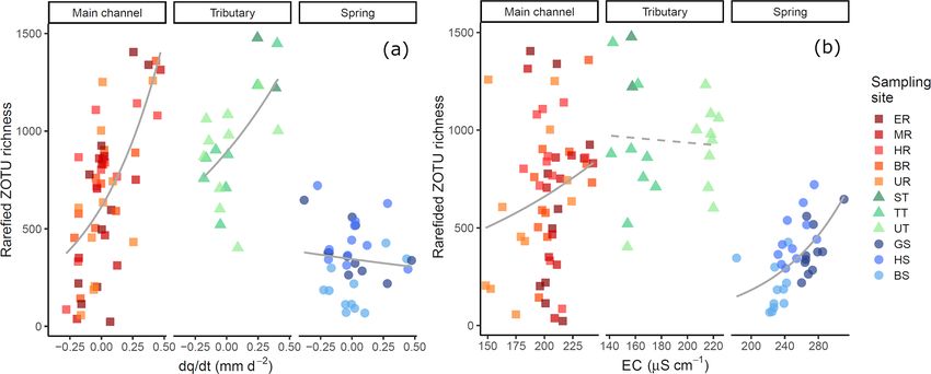
E. Mächler et al.: Environmental DNA in the Vallon de Nant                                                                 741

further apart, which enabled us to identify if communities de-   h = g −1 (Crawley, 2012; Coxe et al., 2009). The identity of
tected with eDNA cluster according to water type or hydro-       the sampling sites was defined as a random effect in an inter-
logic parameters. We used weak ties (stress type 1), allowing    cept model, to take sampling site variability into account.
ties to be broken where equal observed dissimilarities exist        We compared the models with and without interaction of
(Kruskal, 1964a). We calculated the stress of the NMDS ac-       the two explanatory variables (D, W ). The testing of the in-
cording to Kruskal (1964b) as a measure of how well the con-     teraction allows us to identify if the intercept and slope of
figuration matches the observed data. The NMDS was plot-         richness vary according to the water type, whereas a purely
ted for the individual sampling days separately, to observe      additive approach would only allow us to test whether the in-
the development of differences over the sampling season.         tercepts were different, while assuming the slopes were the
   Dissimilarity measures used for the NMDS are based            same. We selected the best model based on a χ 2 test, clas-
on the sequence identities of the ZOTUs and were calcu-          sically used to compare model fits. Since the change in dis-
lated to do a pairwise comparison between sites. We used         charge, dq/dt, was negatively correlated with ZOTU rich-
an unweighted UniFrac (Lozupone and Knight, 2005) as a           ness in springs, we performed a second analysis where we
dissimilarity input to the NMDS, which is based on pres-         replaced dq/dt with EC (E), in the above model. EC is an
ence/absence and the phylogenetic tree (i.e., the evolutionary   indicator of the subsurface exchange that defines the water
relationships among ZOTUs based on their sequence sim-           type of springs likely better than dq/dt. EC was scaled and
ilarity) of the ZOTUs. We further fitted variables of inter-     centered for the model due to large eigenvalue ratios.
est (elevation, EC, water temperature, total daily solar radi-
ation, baseflow, daily snow cover area, dq/dt, δ 18 O, and lc-   2.4.3   Separation of upstream water contribution
ex) onto the NMDS ordination two-dimensional space with a
commonly used method that maximized correlation between          In order to examine the contribution of ZOTUs from up-
the ordination and the corresponding environmental variables     stream springs and tributaries to the richness in the main
(function envfit, R package vegan; Oksanen et al., 2007, ver-    channel downstream, we calculated overlap in ZOTUs. We
sion 2.5-4), to identify the directions towards which the vec-   identified ZOTUs that were unique to samples from one wa-
tors change most rapidly in the presented ordination space.      ter source, shared by only two, or all three water sources.
Next, we focused on ZOTUs that have a taxonomic assign-          If a ZOTU was only found in spring samples or in spring
ment and used the R package indicspecies to identify can-        and main channel samples, but never in any tributary sam-
didate taxa that are statistical significantly associated with   ples over the whole data set, the ZOTU origin was assigned
a particular water type or combinations of those by using a      to springs. If only found in tributaries or in tributaries and
permutation test (De Caceres et al., 2016).                      main channel samples but never in any spring sites, its origin
                                                                 was assigned to tributaries. The ZOTU’s presence in the main
2.4.2   Influence of hydrologic variability on eDNA              channel did not influence this decision, since we assumed the
        diversity                                                main channel contains eDNA of both tributaries and springs,
                                                                 either because it may be shared due to the similar habitat or
Due to the spatiotemporal variability in water sources, Alpine   due to downstream transport of eDNA (Deiner and Altermatt,
catchments are a mosaic of different water types and habitats,   2014; Pont et al., 2018).
indicated by a high range of physical and chemical processes        Next, we partitioned the ZOTUs in main channel samples
(Ward et al., 1999; Tockner et al., 2000). We explored the in-   into those originating from springs and tributaries, providing
fluence of water source contributions on eDNA sampled over       a count of how much springs and tributaries, respectively,
a season associated to two variables: the change in discharge    are contributing to the main channel. We then plotted the
at the catchment outlet, dq/dt and subsurface exchange as re-    relative contributions separately against dq/dt and EC, as
vealed by changes in electrical conductivity (EC) in springs     these were identified as major drivers in our prior analysis
(Laudon, 1997). We used rarefied ZOTU richness, calculated       of ZOTU richness (see Sects. 2.4.1 and 2.4.2). To confirm
for each individual sampling site and time point as a simple     this relationship, we computed a generalized linear model
measure of eDNA diversity. We utilized a generalized linear      (GLM) with the relative contribution (C) as a response vari-
mixed-effect model (GLMM; function glmer in the R pack-          able, dq/dt (D) and the origin of the ZOTU (O) as explana-
age lme4; Bates et al., 2007) with ZOTU richness (R) as the      tory variables:
response variable, change in discharge (D = dq/dt) and the       C = β0 + β1 · D + β2 · O + ,                              (2)
water type (W ) as fixed effects, and the sampling site (S) as
a random effect. The univariate response variable Y = R was      where  comes from a quasi-binomial error distribution. This
modeled with vectors X = [S] and Z = [D, W, DW ] of the          choice results from the fact that (i) binomial error distribu-
explanatory variables associated with the fixed effect (Z) and   tions are appropriate for proportional variables; and (ii) our
the random effect (X). We assumed a Poisson distribution         data set shows overdispersion, i.e., higher variability than
and the conditional mean E(Y |X, Z) = µ = g −1 (η) related       what can be explained by the standard binomial error dis-
to the linear predictor by a log-link function with inverse      tribution. We compared the models with and without inter-

https://doi.org/10.5194/hess-25-735-2021                                        Hydrol. Earth Syst. Sci., 25, 735–753, 2021
742 E. Mächler et al.: Environmental DNA in the Vallon de Nant
action of the two explanatory variables and selected the best parent for two of the tributaries (ST and TT) and to a certain
model with a F test. As before, we also tested a model with extent for the sampling point UR in the main channel.
EC (E) as n explanatory variable replacing D, as it might be The analysis of the physicochemical tracers confirmed the
more important to recover the input of springs: hypothesis underlying the sampling design, namely that the
different sites correspond to different water types with typi-
C = β0 + β1 · E + β2 · O + . (3) cal seasonal patterns of contributions, even if there was some
overlap due to accumulations of different processes. More
explicitly, these sites had different contributions from rain
3 Results and snow inputs at different points in time, as evidenced by
stable isotopes of water, on the one hand, and various ra-
3.1 Confirmation of water typology tios of surface to subsurface flow paths, on the other hand,
as indicated by EC and temperature. Thus, each site had a
Annual precipitation in 2017 was 1760 mm, which is close unique mix of water sources and subsurface contributions,
to the long-term average of 1920 mm over the period and some sites had characteristics of two types. For example,
1961–2017 (minimum 1470 mm, maximum 2600 mm; Me- the uppermost point on the river, UR, seemed to correspond
teoSwiss, 2011). Snowmelt peaked in early June, and snow to the EC and temperature of the main channel sometimes
cover was reduced to 9 % of the watershed area by 1 July but at other times to those of tributaries. Likewise the most
(DOY 181) and reached 0 % on 18 August (DOY 229). Fur- upstream tributary, UT, seemed to have an EC approaching
ther details regarding the hydrometeorological observations that of springs compared to the other tributaries, and the EC
can be found in the Supplement, Sect. S4. In general, the of one spring, BS, is consistently lower than that of the other
three water types (main channel, tributaries, and springs) springs (Fig. S3). Accordingly, we expect the seasonal and
are significantly different from each other according to their spatial biodiversity patterns observed at these sites to be at
physicochemical characteristics. All comparisons of water least partly explained by these different origins and water
temperature were significant (p < 0.05) in mean rank differ- flow paths and, in turn, that eDNA observations might con-
ence according to the Kruskal–Wallis test (Table S6), making vey information on hydrologic processes.
it the best discriminator of the variables besides eDNA (Ta-
ble S7). Springs had the lowest and most stable water temper- 3.2 Differentiation of water type by eDNA
ature; tributaries, including the uppermost point on the main
channel, UR, showed high water temperature variability and There was a higher variability in the number of ZOTUs (i.e.,
were considerably warmer than springs; and the main chan- the richness) found in main channel and tributary sites (i.e.,
nel had intermediary values. Overall, mean EC values were the standard deviation was higher), while sites in springs
higher in springs than other observed water types and gen- were more similar (Fig. 3, Fig. S3). All comparisons of rar-
erally higher at lower elevations. The main channel showed efied ZOTU richness, M–S, M–T, and S–T, were signifi-
mid EC values and a narrow temporal range of EC values, cant (p < 0.05) in mean rank difference according to the
resulting from a mixing of sources (tributaries and springs) Kruskal–Wallis test (Table S6).
throughout the season. Two of the between-water-type com- Next, we focused on the analysis that included the se-
parisons of EC were significant (p < 0.05) in mean rank dif- quence identity of the ZOTUs. The NMDS plot, which uses
ference according to the Kruskal–Wallis test: main channel pairwise comparisons of multidimensional data to represent
to spring (M–S) and spring to tributary (S–T); see Table S6. data in two-dimensional space, resulted in a stress value of
Values of isotopes in the main channel were not consistently 0.132, indicating that the reduced dimensions represent the
intermediary to those in springs and in the tributaries. We data fairly well (Kruskal, 1964a). While spring sites clus-
found significance (p < 0.05) in the mean rank difference of tered slightly apart from main channel sites, this was not the
δ 18 O between the main channel and springs (M–S) and the case for tributary sites that are located at the intersection be-
main channel and tributary (M–T) but not between springs tween the main channel and springs (Fig. 4), indicating that
and tributary (S–T). We found significance in mean differ- the specific ZOTUs of the main channel are phylogenetic
ence of δ 2 H also in those two comparisons, M–S and M–T, closer to the tributary-specific ZOTUs. The arrows in Fig. 4
and in one comparison of lc-ex, M–S. indicate the direction of the fastest change in the environ-
Given the seasonality of the physical processes, the vari- mental variables of EC, δ 18 O, water temperature, and lc-ex,
ables fluctuated over the observation period, though statis- respectively, which were all significant (Table S8), and their
tical confirmation of persistent seasonality was not possible length is proportional to their correlation with the ordination
with a single season of data. Enrichment and depletion of the of the genetic data (Oksanen et al., 2007). EC is the most
stable isotope concentrations in streamflow are mainly deter- important explanatory variable (i.e., it has the longest arrow
mined by contributions of snow (including snowmelt) ver- in Fig. 4), followed by water temperature, lc-ex, and finally
sus rainfall (Fig. 2). The alternation of sources is visible as a δ 18 O. The NMDS plots separated by sampling day (Fig. S5)
large range in isotopic ratios (Fig. S3) and is particularly ap- show that in May and June (DOY 136 and 164), both trib-
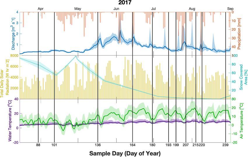
Hydrol. Earth Syst. Sci., 25, 735–753, 2021 https://doi.org/10.5194/hess-25-735-2021E. Mächler et al.: Environmental DNA in the Vallon de Nant 743 Figure 2. Discharge (blue, upper), precipitation (red upper), total solar radiation (yellow, middle), snow cover area (cyan, middle), water temperature (purple, lower), and air temperature (green, lower) for the sampling season (2017). Meteorological variables were averaged over the catchment area, whereas water discharge and temperature were measured at the outlet (MR/ER). Shaded areas show the range of values of temperature within a day at the four stations (air, green) and at the outlet (water, purple) and the range of flow at the outlet for discharge and show the error of the snow-covered area estimated from satellite data. Sampling days are indicated as vertical black lines with the corresponding day of the year on the lower axis. utaries and the main channel are more similar to each other confirming traditional observations (Milner and Petts, 1994). compared to later in the season. The similarly low isotope It is a common challenge of eDNA metabarcoding for the values across all sites (δ 18 O = 11.9 ‰, range 1.4 ‰ on DOY COI gene that only a low proportion of ZOTUs have an asso- 164) allow us to attribute early season homogeneity in eDNA ciated taxonomic name (here 3 %, representing only 5 % of to the dominance of snowmelt, which flushes the system and the reads), which largely results from a lack of reference data reduces inter-site variability. In contrast, in the late season (Weigand et al., 2019). Thus, all further analysis were done (DOY 220), there was the highest range of water isotope val- at the level of ZOTUs, irrespective of whether they had a ues (δ 18 O, 3.05 ‰) across all sites (Fig. 3), suggesting more taxonomic name assigned to them or not, which is suggested mixing of water originating as different types of precipita- to be the future avenue of metabarcoding (Apothéloz-Perret- tion and subsequent different trajectories of storage before Gentil et al., 2017; Cordier et al., 2018). being released as streamflow. However, the persistent clus- tering in eDNA suggests that the flood event in early August 3.3 Influence of hydrologic variability on eDNA (see Fig. S5, DOY 215) equalized the detected eDNA com- diversity munity of tributaries and the main channel for this day, while it was spread wider the sampling days before (DOY 207) and The link between environmental variability in the differ- after (DOY 220). ent water sources and detected richness was pronounced: A total of 3 % (286) of ZOTUs had a taxonomic assign- both change of discharge and EC affected detected richness ment to genus level (Supplement Sect. S6), of which 14 ZO- (Fig. 5a respectively b); and the best model included the in- TUs were significantly associated with the main channel, 3 teraction of the fixed effects for both the model with dq/dt with springs, and 26 with tributaries according to the indi- and the model with EC (Table S10). The first model, includ- cator analysis (Table S9). A total of 17 ZOTUs were asso- ing dq/dt, revealed that the fixed effects and their interaction ciated with tributaries and main channel sites. Multiple ZO- were significant (Table 1; see Table S11 for results of random TUs assigned to the genus of Diamesa were associated with effects). However, water source is a factorial variable, and the the main channel or both the main channel and tributaries, individual sources did not show the same response: the inter- https://doi.org/10.5194/hess-25-735-2021 Hydrol. Earth Syst. Sci., 25, 735–753, 2021
744                                                                      E. Mächler et al.: Environmental DNA in the Vallon de Nant

Figure 3. Variation in δ 18 O (a), δ 2 H (b), lc-ex (c), EC (d), temperature (e), and rarefied ZOTU richness (f) for the individual sampling sites
over the field season (given as day of the year). The sampling sites in the legend are clustered based on the water source and within the
cluster ordered from low to high elevation. The figure legend corresponds exactly to that in Fig. 1, and the x axis corresponds exactly to that
in Fig. 2.

                                                                            cept (−0.637) and the slope (−2.055) for the spring samples
                                                                            are negative compared to the main channel, indicating an in-
                                                                            verse effect of dq/dt on the richness detected in springs. The
                                                                            slope for tributary sites is smaller compared to the main chan-
                                                                            nel sites but still resulting in a positive relationship of rich-
                                                                            ness and dq/dt. The second model, including EC instead of
                                                                            dq/dt as a fixed effect, identified all fixed effects and their
                                                                            interaction to be significant, except the interaction of EC and
                                                                            tributary sites.

                                                                            3.4   Separation of upstream water contribution

                                                                            Over the whole sampling campaign, 79.2 % of ZOTUs found
                                                                            in tributaries were recovered in the main channel, compared
                                                                            to 77.0 % found in springs and the main channel (Fig. 6).
                                                                            Over all ZOTUs, we found 1374 ZOTUs (14.3 %) that were
Figure 4. Community composition in the main channel, tribu-                 detected only in spring sites but never tributaries and 3221
taries, and springs. Non-metric multidimensional scaling (NDMS)             ZOTUs (33.5 %) that were exclusively assigned to tributary
analysis of communities based on UniFrac dissimilarities (stress =
                                                                            sites. The best generalized linear model for dq/dt included
0.132, indicating a fair representation of the data in the reduced di-
                                                                            the interaction with the origin of the ZOTUs (Table S12).
mensions). The axis represent the dimensions 1 (NMDS1) and 2
(NMDS2), respectively. Ellipses represent a 95 % confidence inter-          Only the contribution from ZOTUs originating in tributaries
val.                                                                        to the main channel had a significant interaction with dq/dt,
                                                                            while no significant interactions were observed for ZOTUs
                                                                            originating from springs (Table 2, Fig. 6b). In contrast, the

Hydrol. Earth Syst. Sci., 25, 735–753, 2021                                                     https://doi.org/10.5194/hess-25-735-2021
E. Mächler et al.: Environmental DNA in the Vallon de Nant 745
Table 1. Results from the generalized linear mixed model fit by maximum likelihood (Laplace approximation) for fixed effects; asterisks
stand for the interaction. Note that the water source is a factor with three levels (main channel, spring, and tributary). The estimate of the
slope (relationship) in the model is indicated.
Model Fixed effects Estimate SE z value p value
dq/dt Main channel (intercept) 6.407 0.093 68.888 < 0.001
dq/dt (slope) 1.791 0.026 69.582 < 0.001
Spring −0.637 0.152 −4.192 < 0.001
Tributary 0.434 0.152 2.855 0.0043
dq/dt*spring −2.055 0.053 −38.485 < 0.001
dq/dt*tributary −1.128 0.048 −23.668 < 0.001
EC Main channel (intercept) 6.569 0.090 73.092 < 0.001
EC (slope) 0.201 0.010 20.335 < 0.001
Spring −1.183 0.149 −7.946 < 0.001
Tributary 0.549 0.149 3.705 < 0.001
EC*spring 0.156 0.024 6.517 < 0.001
EC*tributary −0.027 0.021 −1.272 0.203
Figure 5. Rarefied ZOTU richness plotted against dq/dt (a) and EC (b). The sampling sites in the legend are clustered based on the water
source and within the cluster ordered from low to high elevation. Solid lines indicate significant interactions of fixed effects, and the dashed
line indicates significant relationship of the fixed effects and the response variable only (without observed significant interaction). Smoothing
lines are based on the GLM function. Note that the scale of the x axis for EC (b) varies by water type.
best model with EC, which was more correlated with rich- taries, especially compared to springs, and showed less vari-
ness in springs, did not include an interaction term (Table 2, ation over time in tributaries than the main channel. Below,
Fig. 6c). we further elaborate on what we learn about the hydrology
of the study site from eDNA observations and on the rela-
tionship between eDNA and the two physical variables that
4 Discussion were most strongly associated with it, namely the change in
discharge dq/dt and EC. Overall, in response to our own spe-
Our results highlight that eDNA can provide additional in- cific questions and hypotheses, we found that the eDNA sig-
sights regarding the water type and origin when accompa- nal not only provided unique biological information, but also
nied by observations of naturally occurring physicochemical partially discriminated water types, reflected hydrologic vari-
tracers. Additionally, eDNA delivers information about time ability, and was determined by upstream contributions.
points of high connectivity between the sampling sites in a
hydrologic highly diverse Alpine system. Thereby, it com- 4.1 Differentiation of water type by eDNA
plements the classical observation of stable isotopes of wa-
ter, water temperature, and EC. The measure of taxonomic Our analysis showed that the eDNA composition of the three
richness assessed by eDNA showed highest values in tribu- water types was indeed different but not to a level that made
https://doi.org/10.5194/hess-25-735-2021 Hydrol. Earth Syst. Sci., 25, 735–753, 2021746 E. Mächler et al.: Environmental DNA in the Vallon de Nant
Figure 6. Venn diagram for the three sampled water sources; overlapping areas depict shared ZOTUs between water sources (a). Values
indicate the numbers of ZOTUs in the given section, and the size of the circles is weighted by the number of ZOTUs. Relative contribution
of ZOTUs from tributaries (green) or springs (blue) to samples in the main channel against dq/dt (b) and EC (c). The solid line indicates
significant interactions of fixed effects, the dashed lines indicate significant relationships of both fixed effects and response variable only
(without significant interaction), and the dotted line indicates only the significant relationship of one fixed effect. Smoothing lines are based
on the GLM function.
Table 2. GLM results for response variables based on a t test; asterisks stand for the interaction. Note that the origin of the ZOTU is a factor
with two levels (spring and tributary).
Model Coefficients Estimate SE t value p value
dq/dt Spring (intercept) −2.700 0.052 −51.548 < 0.001
dq/dt −0.498 0.298 −1.673 0.09724
Tributary 1.386 0.061 22.685 < 0.001
dq/dt *tributary 1.147 0.340 3.368 0.00106
EC Spring (intercept) −2.377 0.270 −8.790 < 0.001
EC −0.001 0.001 −1.255 0.212
Tributary 1.416 0.064 22.063 < 0.001
them entirely distinct. In fact, we always expect a portion of sity work (e.g., Milner and Petts, 1994; Ward, 1994; Brown
the eDNA signal that is non-informative on the water types, et al., 2003). Interestingly, phylogenetic community compo-
and this overlap can be explained by either shared species sition of the tributaries is between the main channel and the
compositions due to ecological connectivity between sites spring sites, represented in the intermediate position of the
(Pringle, 2003; Bracken and Croke, 2007) and/or by transport clustering in the NMDS. The transport of eDNA is not able
of eDNA between hydrologically connected sites, i.e., down- to override these differences; otherwise we would expect the
stream in the main channel or laterally through groundwa- main channel to cluster between the tributary and the spring
ter exchange with the hyporheic zone (Bracken et al., 2013). sites. By monitoring over a season, we identified time points
Even through a hydrologic lens, these three water types are of greater and lesser homogeneity among sites according to
not entirely distinct; for example, groundwater contributes the eDNA community. This is consistent with the different
to the flow in the tributaries and main channel. The feasi- hydrologic characteristics: while the main channel and tribu-
bility of using eDNA data to disentangle different hydro- taries resembled each other more (i.e., were more connected)
logic contributions in low-land streams, specifically inflows on days with increased precipitation or snowmelt (e.g., DOY
from wastewater treatment plants into natural streams, has re- 136, 164, or 215), springs fed by groundwater were more
cently been demonstrated (Mansfeldt et al., 2020). Thus, in stable over time and showed no reaction. eDNA provides
a context of completely distinct water sources, source track- promising new insights into the temporal evolution of the
ing with DNA from microorganisms is possible but may be connectivity of the stream network system, a key to assessing
more challenging in natural Alpine streams with overlapping dominant hydrologic flow paths.
signals (Wilhelm et al., 2013). Future studies might investigate how community composi-
We identified EC and temperature as the two most impor- tion could be exploited to enhance knowledge about ecosys-
tant indicators for the community clustering over all samples. tem processes. However, our analysis was restricted to ZO-
This corroborates previous, classical Alpine stream biodiver- TUs identity, as currently the assignment of species names
Hydrol. Earth Syst. Sci., 25, 735–753, 2021 https://doi.org/10.5194/hess-25-735-2021You can also read