A Compact Rayleigh Autonomous Lidar (CORAL) for the middle atmosphere - Recent
←
→
Page content transcription
If your browser does not render page correctly, please read the page content below
Atmos. Meas. Tech., 14, 1715–1732, 2021
https://doi.org/10.5194/amt-14-1715-2021
© Author(s) 2021. This work is distributed under
the Creative Commons Attribution 4.0 License.

A Compact Rayleigh Autonomous Lidar (CORAL) for
the middle atmosphere
Bernd Kaifler and Natalie Kaifler
Deutsches Zentrum für Luft- und Raumfahrt, Institut für Physik der Atmosphäre, Oberpfaffenhofen, Germany

Correspondence: Bernd Kaifler (bernd.kaifler@dlr.de)

Received: 21 October 2020 – Discussion started: 26 October 2020
Revised: 14 January 2021 – Accepted: 18 January 2021 – Published: 2 March 2021

Abstract. The Compact Rayleigh Autonomous Lidar                  1   Introduction
(CORAL) is the first fully autonomous middle atmosphere li-
dar system to provide density and temperature profiles from      For several decades, light detection and ranging (LiDAR;
15 to approximately 90 km altitude. From October 2019 to         also spelled lidar) has been used to profile the atmosphere
October 2020, CORAL acquired temperature profiles on 243         and retrieve information on aerosols, trace gases, and at-
out of the 365 nights (66 %) above Río Grande, southern          mospheric density, temperature, and wind (see, e.g., Fujii,
Argentina, a cadence which is 3–8 times larger as com-           2005). Following the invention of the laser, first observations
pared to conventional human-operated lidars. The result is       of tropospheric clouds were reported in the early 1960s. Soon
an unprecedented data set with measurements on 2 out of 3        thereafter more powerful lasers and sensitive detectors led
nights on average and high temporal (20 min) and vertical        to detection of stratospheric aerosols by lidar (e.g., Collis,
(900 m) resolution. The first studies using CORAL data have      1965; Schuster, 1970). But it took until the early 1980s be-
shown, for example, the evolution of a strong atmospheric        fore the lidar technology was developed far enough to enable
gravity wave event and its impact on the stratospheric cir-      measurements of atmospheric density and temperature in the
culation. We describe the instrument and its novel software      mesosphere (Hauchecorne and Chanin, 1980). In contrast to
which enables automatic and unattended observations over         their tropospheric counterparts, the mesospheric lidars were
periods of more than a year. A frequency-doubled diode-          rather complex experiments requiring a great deal of labor
pumped pulsed Nd:YAG laser is used as the light source, and      to set up and operate, with some systems filling entire build-
backscattered photons are detected using three elastic chan-     ings (von Zahn et al., 2000). Hence, these lidars were run
nels (532 nm wavelength) and one Raman channel (608 nm           only during campaigns, or, e.g., in the case of stations be-
wavelength). Automatic tracking of the laser beam is realized    longing to the Network for the Detection of Atmospheric
by the implementation of the conical scan (conscan) method.      Composition Change, operation was limited to certain days
The CORAL software detects blue sky conditions and makes         per week when the weather forecast looked favorable and
the decision to start the instrument based on local meteoro-     trained operators were available. The intermittent operation
logical measurements, detection of stars in all-sky images,      not only limited the amount of data but also made statistical
and analysis of European Center for Medium-range Weather         studies that require a dense temporal sampling of the atmo-
Forecasts Integrated Forecasting System data. After the in-      sphere, e.g., the investigation of the evolution of atmospheric
strument is up and running, the strength of the lidar return     gravity wave events (e.g., Kaifler et al., 2020), next to im-
signal is used as additional information to assess sky condi-    possible. Gravity wave climatologies which do not require a
tions. Safety features in the software allow for the operation   dense sampling were published by, e.g., Wilson et al. (1991),
of the lidar even in marginal weather, which is a prerequisite   Sivakumar et al. (2006), Rauthe et al. (2008), Li et al. (2010),
to achieving the very high observation cadence.                  Mzé et al. (2014), and Kaifler et al. (2015b).
                                                                    In recent years, a number of autonomous tropospheric li-
                                                                 dar systems have been developed to address the shortcomings
                                                                 of the earlier manually operated instruments and increase

Published by Copernicus Publications on behalf of the European Geosciences Union.
1716                                                       B. Kaifler and N. Kaifler: Compact Rayleigh Autonomous Lidar

the data output (Goldsmith et al., 1998; Reichardt et al.,               analysis of the temperature structure on timescales from
2012; Strawbridge, 2013; Engelmann et al., 2016; Straw-                  years to minutes.
bridge et al., 2018). But until today, to the knowledge of the
authors, no attempts were made to build autonomous mid-               3. A computer in charge of operating the lidar removes any
dle atmosphere lidars. There may have been several factors               sampling biases caused by the work schedule of human
contributing to the stalled development. First, lidars capable           operators, for example less measurements during week-
of sounding the mesosphere require a much higher sensitiv-               ends and holidays.
ity given the exponential decrease in air density with alti-
                                                                  Given these compelling advantages, it is almost incompre-
tude. Consequently, mesospheric lidars use powerful lasers,
                                                                  hensible why, in the past, little effort has been undertaken to
large aperture receiving telescopes, and highly efficient re-
                                                                  develop autonomous middle atmosphere lidar systems. One
ceivers, which makes some of the solutions generally used
                                                                  of the reasons is certainly that lidar scientists and engineers
in the development of autonomous tropospheric lidars im-
                                                                  are often not well trained in software design and software de-
practical, as, for instance, a window covering the telescope
                                                                  velopment. As we will show later, it takes considerable effort
to protect it from the environment. Second, because of the
                                                                  and time to develop and test the software required for au-
technical challenges and lower interest in the middle atmo-
                                                                  tonomous lidar operation. In the case of CORAL, the hard-
sphere as compared to the troposphere, there are only a few
                                                                  ware of the instrument is rather unexceptional, and it is in-
groups operating middle atmosphere lidar instruments.
                                                                  deed the software which contains most of the complexity of
   The primary objective of the Compact Rayleigh Au-
                                                                  the system. Another reason is that operators are required for
tonomous Lidar (CORAL) is the demonstration of a fully
                                                                  safety reasons at some sites.
autonomous lidar system which can be used for studying
                                                                     The purpose of this paper is threefold. First, we want
atmospheric dynamics in the stratosphere and mesosphere.
                                                                  to demonstrate the functionality of an autonomous operated
That the instrument should be capable of fully automatic ob-
                                                                  middle atmosphere lidar. Second, given the advances in com-
servations was not seen as a practical feature but rather as
                                                                  puter power and software development tools, this paper will
pure necessity resulting from the lack of human effort to
                                                                  demonstrate that the building of an autonomous lidar instru-
operate the instrument. For the same reason, the instrument
                                                                  ment is not overly complicated. Third, as we will argue in
should require only a bare minimum of maintenance work.
                                                                  the discussion (Sect. 5), the large and continuous data sets
In other words, the instrument should happily sit by itself,
                                                                  produced by autonomous instruments facilitate advances in
monitor itself, and collect atmospheric measurements when-
                                                                  science that are hardly possible with conventional human-
ever weather conditions allow for optical soundings. Human
                                                                  operated lidar instruments. Following this agenda, we de-
interaction should be limited to approximately weekly down-
                                                                  scribe the lidar instrument in Sect. 2, followed by the descrip-
loads of scientific data and yearly maintenance. Moreover,
                                                                  tion of the software used for autonomous lidar operation in
CORAL should be transportable, fully independent of infras-
                                                                  Sect. 3. In Sect. 4, we briefly discuss our implementation of
tructure expect for electrical power, robust enough to with-
                                                                  the temperature retrieval.
stand environmental conditions from the tropics to the Arc-
tic and Antarctic, easy to replicate, and in relative terms low
cost. In short, we wanted to develop a lidar system which         2    The lidar instrument
can be set up at some remote location and left there for years
collecting atmospheric data, much like ceilometers are used       Development of CORAL started in 2014 as a copy of the Ger-
today by the weather services. If such a system was possible,     man Aerospace Center’s first mobile middle atmosphere lidar
it would surely mark the transition from the conventional,        system, TELMA (Temperature Lidar for Middle Atmosphere
laboratory style and labor-intensive lidar systems commonly       Research), which was employed with much success dur-
in use today and run by lidar experts to a new generation of      ing the deep propagating gravity wave experiment (DEEP-
operational lidar systems which can be run by experts and         WAVE) field campaign in New Zealand (Fritts et al., 2016;
non-experts alike. There are several benefits expected from       Kaifler et al., 2015a; Ehard et al., 2017; Taylor et al., 2019;
such a new generation of lidars.                                  Fritts et al., 2019). CORAL measures atmospheric density
                                                                  in the altitude range 15–95 km and thus covers most of the
 1. As the cost of lidar operators contribute significantly to
                                                                  stratosphere and mesosphere. The system uses a pulsed laser
    the operating costs of conventional lidars, the use of au-
                                                                  at 532 nm wavelength as light source and a receiver equipped
    tonomous systems will bring the cost per operating hour
                                                                  with several channels for detecting both elastic scattering and
    down. Lower costs will enable a more widespread use
                                                                  inelastic scattering at 608 nm wavelength. Atmospheric tem-
    of lidar systems for atmospheric research and climate
                                                                  perature is retrieved by hydrostatic integration of the mea-
    monitoring.
                                                                  sured density profiles (Hauchecorne and Chanin, 1980).
 2. Not having to rely on human operators to acquire sound-          The lidar instrument is integrated into an 8 foot (2.4 m)
    ings facilitates the collection of large and continuous       steel container (see Fig. 1) which serves both as transport
    data sets, thus offering new possibilities for statistical    container and enclosure during lidar operation. The container

Atmos. Meas. Tech., 14, 1715–1732, 2021                                             https://doi.org/10.5194/amt-14-1715-2021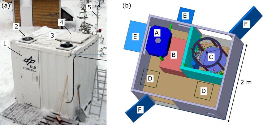
B. Kaifler and N. Kaifler: Compact Rayleigh Autonomous Lidar                                                                 1717

is divided into two compartments: an air-conditioned room          over the altitude range of 40–50 km as a function of motor
accommodates the transmitter, receiver, and data acquisition       position. Repeated scans are performed and measurements
systems, while the telescope is located in a separate room         averaged in order to reduce the effect of potential changes
with a large hatch in the roof for direct access to the sky. The   in atmospheric transmission during the scans. The focal po-
technical specifications of the lidar instrument are summa-        sition is determined as the position with the maximum lidar
rized in Table 1.                                                  signal.
                                                                      With the bistatic setup, full geometric overlap between the
2.1   Transmitter                                                  laser beam and the telescope FOV is achieved at approxi-
                                                                   mately 5 km altitude. However, range-dependent defocusing
Figure 2 shows the schematics of the optical paths inside the      of the telescope causes the overlap function to vary slightly
lidar instrument. The laser (SpitLight DPSS 250-100 from           with altitude. This variable overlap results in a bias in re-
InnoLas GmbH) is a diode-pumped Nd:YAG master oscilla-             trieved temperature profiles of less than −0.4 K for altitudes
tor power amplifier system operating at 1064 nm wavelength         above 40 km which increases to −0.95 K at 15 km altitude
and 100 Hz pulse repetition frequency. It delivers 120 mJ per      (see Sect. S2 in the Supplement).
pulse after conversion to the second harmonic at 532 nm               The optical bench of the receiver resides in a four-unit
wavelength. The remaining infrared light is separated and          19 in. (482.6 mm) rack mount enclosure. The optical fiber en-
subsequently dumped using a dichroic mirror and water-             ters the enclosure at the back side and terminates in front of
cooled beam dump. A folding mirror mounted on a fast               a mechanical chopper with three slits rotating at 100 revo-
tip/tilt piezo actuator with a 7 mrad angular range directs the    lutions per second. The firing time of the laser is synchro-
green beam towards a 2× beam expander which reduces the            nized with the rotation of the chopper such that laser light
beam divergence to approximately 170 µrad and the pointing         scattered in the lower 14 km of the atmosphere is blocked
jitter to < 50 µrad full angle. The resulting effective beam       by the chopper blades and does not hit the sensitive detec-
divergence is thus < 220 µrad or approximately half of the         tors. As shown in Fig. 2, after passing through the collima-
telescope field of view (FOV). Finally, the beam exits the         tion optics, the collimated beam is spectrally divided into
laser box through an anti-reflection coated window. A mo-          two parts by a dichroic mirror, separating the elastic scat-
torized mirror located in the telescope compartment of the         tering at 532 nm wavelength and the nitrogen rotational Ra-
container directs the laser beam into the sky at a position that   man scattering at ∼ 608 nm wavelength. The Raman scatter-
is approximately 0.4 m offset from the optical axis of the re-     ing is detected using a photomultiplier (Hamamatsu H7421;
ceiving telescope.                                                 approximately 35 % detection efficiency at 600 nm) with a
                                                                   3 nm wide interference filter (80 % peak transmission, out-
2.2   Receiver                                                     of-band blocking optical depth, OD, > 6) mounted in front.
                                                                   The dichroic mirror has a transmission of 1.2 % at 532 nm
The backscattered light is collected using a 63.5 cm diameter      wavelength, and this results in a total blocking of the elastic
parabolic f/2.4 mirror with a spot size of ∼ 60 µm. An optical     scattering in the Raman channel of OD ∼ 8.
fiber (type FG550LEC; 550 µm core diameter, 0.22 numeri-              In order to increase the dynamic range of the detection,
cal aperture) mounted on the focal plane guides the collected      the beam containing the elastic scattering is further split into
light to the receiver. The fiber mount consists of a spring-       three beams with a splitting ratio of approximately 92.0 :
loaded piston traveling inside a fixed tube with the piston        7.4 : 0.6, i.e., the detector of the far channel sees 92 % of
pushing against a linear motor (Thorlabs Z812). With the           the light, while only 0.6 % of the light reaches the low chan-
help of the motor, the position of the fiber end can be adjusted   nel. Both the high- and mid-channel detectors are avalanche
in the z direction with ∼ 2 µm resolution, thus facilitating the   photo diodes (APDs) operated in Geiger mode (SPCM-
easy adjustment of the telescope focus. The outer tube is held     AQRH-16 from Excelitas; ∼ 50 % detection efficiency at
by a three-legged spider mounted on an aluminum ring with a        532 nm wavelength) with 0.8 nm wide interference filters
diameter slightly larger than the mirror. The ring is supported    (83 % peak transmission) mounted in front. The APDs are
by six vertical carbon fiber tubes that connect it to the base     gated to limit peak count rates to about 5 MHz. The low
plate holding the telescope mirror, and the whole telescope        channel detector is again a photo multiplier tube (Hamamatsu
assembly sits on adjustment screws that allow the telescope        H12386-210) with a 3 nm wide cost-efficient interference fil-
to be pointed to zenith. The use of carbon fiber tubes results     ter (60 % peak transmission).
in the high thermal stability of the telescope. A 50 K change
in temperature causes the focal point to shift by 160 µm in the    2.3   Data acquisition and control
vertical. As shown in the Supplement, this shift has a negli-
gible impact on the fiber coupling performance. During the         The data acquisition system comprises three units: the ac-
setup of the instrument, the optimum position is determined        quisition computer, the control electronics, and the MCS6A
by slowly moving the fiber end up and down using the motor         photon counter. The MCS6A produced by FAST ComTec
and recording the strength of the lidar return signal integrated   GmbH is a five-channel multi-event digitizer with 800 ps res-

https://doi.org/10.5194/amt-14-1715-2021                                             Atmos. Meas. Tech., 14, 1715–1732, 2021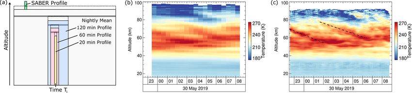
1718 B. Kaifler and N. Kaifler: Compact Rayleigh Autonomous Lidar
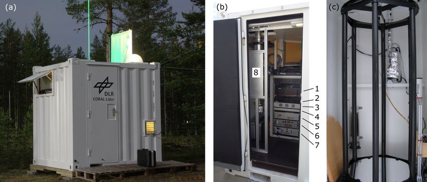
Figure 1. (a) A picture of the CORAL instrument container taken during lidar measurements at the Sodankylä Geophysical Observatory,
Finland, in September 2015. (b) A view into the container through the open front door showing the lidar rack with the receiver (1), data
acquisition computer (2), lidar electronics (3), telescope electronics (4), laser head (5), laser power supply (6), laser cooler (7), and an
Advanced Mesospheric Temperature Mapper (AMTM) as a guest instrument (8). (c) The telescope in the back of the container. Pictures by
N. Kaifler.
Table 1. A summary of the lidar technical specifications.
Laser 120 mJ pulse energy at 532 nm wavelength, 100 Hz pulse rate
Telescope 63.5 cm diameter, 361 µrad field of view, 60 µrad (2σ ) spot size
Receiver Three elastic channels and one Raman channel (608 nm wavelength)
Data acquisition Single pulse acquisition with 800 ps (1.2 cm) resolution
Data products Temperature profiles 15–90 km altitude; resolution 900 m × 20 min (vertical × time);
higher resolutions possible for reduced altitude ranges
olution. It converts the electrical pulses coming from the de- tectors and relays that are controlled by the FPGA for switch-
tectors to timestamps indicating the elapsed time since the ing the detectors on and off.
firing of the laser. The data acquisition software running on
the computer reads out the MCS6A after each laser pulse 2.3.1 Automatic tracking of the laser beam
and stores the timestamps on solid state drives for postpro-
cessing, as well as sorts them into histograms for displaying
One problem with container-based lidar systems is the lim-
the photon count profiles in real-time.
ited thermal stability. When the telescope hatch opens and
Trigger signals for the laser, chopper, and APD gating are
the telescope compartment cools down, thermal drifts re-
produced by the control electronics. Its core is a National
sult in misalignment between the telescope boresight and the
Instruments sbRIO-9633 embedded single-board computer
laser beam. This drift is especially problematic for lidar sys-
with a field-programmable gate array (FPGA). The trigger
tems which use narrow field of views in the order of few
chain of the lidar is implemented in the FPGA, and pro-
hundred microradians for low background noise, and active
grammable delays in the outputs allow for adjusting the tim-
tracking of the laser beam position is usually required. Two
ing between the signals, for example, setting the phase and
methods are commonly used to track the laser beam. With
thus the opening altitude of the chopper and controlling the
manual tracking, an operator performs a quadrant search by
gating of the APDs. Analog outputs of the sbRIO drive the
moving the laser beam by a small angle in alternating direc-
tip/tilt piezo mirror inside the laser through high voltage am-
tions while monitoring the strength of the lidar return signal.
plifiers also located in the electronics box. Prior to outputting
When the scan is completed, the beam angles which yield
the analog signals, the drive signals for the piezo mirror are
the strongest lidar signal are chosen as the new beam posi-
conditioned and limited in bandwidth by digital filters imple-
tion. The search is repeated at regular intervals, e.g., hourly.
mented in the FPGA to prevent the mirror from overshooting
Innis et al. (2007) describe an automatic autoguiding system
the target position and excitation of resonant modes. Finally,
which uses a camera looking through the receiving telescope
the electronics box also houses the power supplies for the de-
to image the spot of the laser beam in the atmosphere at a
certain altitude. A piece of software analyzes the images and
Atmos. Meas. Tech., 14, 1715–1732, 2021 https://doi.org/10.5194/amt-14-1715-2021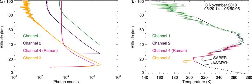
B. Kaifler and N. Kaifler: Compact Rayleigh Autonomous Lidar                                                                        1719

Figure 2. Schematics of the lidar instrument and optical paths.

computes the beam position. Any deviation from the prede-
termined target position is nulled by a servo loop. The tar-
get needs to be found by other means, e.g., manual search.
While the latter method is suitable for an automatic lidar like
CORAL, we opted to implement the conscan method that
is widely used for tracking spacecraft (see e.g., Gawronski
and Craparo, 2002). Its main advantages over the autoguid-
ing method (Innis et al., 2007) are the possibility to evaluate
the lidar signal for tracking purposes in the stratosphere and
thus well above any potential cloud layer and that there is no
requirement for a predetermined target position. In particular,
the resilience to clouds is attractive as CORAL is designed to
operate in marginal weather conditions. To our knowledge,
this is the first application of conscan to mesospheric lidars.
   The basic principle of conscan is depicted in Fig. 3. A scan
mirror rotates about the x and y axes in a sinusoidal motion,
causing the laser beam to rotate around the telescope bore-             Figure 3. The coordinate system of the scan mirror.
sight in a conical scan (see Fig. 4). If the center of the cone is
offset from the boresight of the telescope, the angle between
the laser beam and the telescope boresight 2 periodically be-           where ϑs denotes the phase angle with the largest demodu-
comes smaller and larger due to the conical motion of the               lated lidar return signal.
laser beam. Assuming the offset of the cone is sufficiently                Equation (1) tells us in which direction we have to move
large, the modulation of 2 leads to an incomplete overlap               the laser beam in order to achieve complete overlap, but we
between the telescope FOV and the laser beam. This in turn              do not know how far along es we have to go in order to reach
causes a modulation in the signal strength of the lidar return          the point defined by s. Based on the data at hand, there is no
signal which can be demodulated and the information used                way to determine the scaling factor l in the relation s = les ,
to infer the direction the axis of the cone needs to be shifted         but we can estimate l from the amplitude of the conscan sig-
to in order to obtain a complete overlap. An example of such            nal. For simplicity, we initially assume a perfect lidar pro-
a demodulated signal is shown in Fig. 5. Looking at the ge-             ducing noise-free measurements. Let us consider the situa-
ometry depicted in Fig. 6, it becomes clear that maximum                tion in which the mean 2 equals half of the telescope FOV
overlap is achieved if vector r points in the same direction as         and the amplitude of the modulation signal driving the con-
vector s. The corresponding direction in the coordinate sys-            scan, |r|, is so large that the lidar return signal oscillates be-
tem of the scan mirror is given by the vector                           tween zero (no overlap) and a maximum (complete overlap)
                                                                        and that the demodulated conscan signal, in the following
                                                                        denoted as A, shows oscillations between zero and one. This

           cos ϑs                                                       can be achieved only if |r| also equals half of the telescope
es =                ,                                             (1)   FOV. When the modulation amplitude or mean 2 are smaller,
           sin ϑs

https://doi.org/10.5194/amt-14-1715-2021                                                  Atmos. Meas. Tech., 14, 1715–1732, 2021
1720                                                         B. Kaifler and N. Kaifler: Compact Rayleigh Autonomous Lidar

                                                                    Figure 6. Position of the laser beam and telescope boresight during
Figure 4. Angular modulation of the scan mirror.                    a conscan (adapted from Gawronski and Craparo, 2002).

                                                                    that a more accurate relation can be derived from the calcu-
                                                                    lation of the geometric overlap function based on the actual
                                                                    beam profile of the laser, but the approximation in Eq. (3) is
                                                                    sufficient for our purposes. After a conscan is completed, the
                                                                    orientation of the conical scan is updated by adding ŝ to the
                                                                    current orientation and a new conscan is started. This cycle
                                                                    of scanning and updating of the beam pointing is constantly
                                                                    repeated during the lidar measurement, causing the mean po-
                                                                    sition of the laser beam to track the telescope FOV.
                                                                       In our implementation of conscan, we set |r| = 43 µrad
                                                                    and the speed of the conical motion to 0.4 Hz. Furthermore,
                                                                    we bin the conscan signal A using bins of 18◦ width and av-
                                                                    erage it over 20 s, i.e., 8 revolutions of the laser beam and
Figure 5. Example of a demodulated conscan signal acquired with     100 laser pulses per bin. The averaging reduces the impact
CORAL. The dashed line indicates the mean signal that would be      of statistical variations in atmospheric transmission (e.g.,
obtained in the case of a perfect beam overlap and no modulation.   caused by clouds) and fluctuations in laser power. Figure 5
                                                                    shows such an averaged conscan signal that was acquired on
                                                                    3 November 2019 05:15 UTC in the altitude range 45–55 km
the minimum lidar return signal must be larger than zero as
                                                                    using the far channel detector. The demodulated signal con-
there is always a partial overlap. In this case, A contains a
                                                                    tains a significant noise portion, but a sinusoidal modulation
nonzero offset c, and the amplitude of the sinusoidal part a
                                                                    with a maximum at about 75◦ is nevertheless evident. In or-
is smaller than 1, and we can rewrite A as
                                                                    der to get a better estimate of the amplitude and phase of
A = c + a cos (ϑ − ϑs ) .                                    (2)    the maximum, we perform a sinusoidal fit using the MP-
                                                                    FIT algorithm (Markwardt, 2009). For the example shown
On the other hand, for the other extreme case in which the          in Fig. 5, we obtained values of a = 0.0105 and ϑs = 71.5◦
conscan modulation and mean 2 are so small that the laser           which, according to Eq. (3), cause a shift of 3.5 µrad towards
beam is always completely inside the telescope FOV, we ex-          the telescope boresight when the conscan algorithm is exe-
pect no variation in A and hence a = 0. Thus, the amplitude         cuted. Figure 7 shows mean angles of the scan mirror for a
a can be used as an estimate of the overlap. For simplicity,        4 h long lidar measurement. After startup of the instrument,
in the following we assume a linear relationship and approx-        the warming-up of the laser and cooling-down of the tele-
imate s as                                                          scope compartment of the container caused a drift of about
         (
           10a|r|es if a < 0.1                                      300 µrad (distance in both axes) during the first hour. That is
s ≈ ŝ =                        .                        (3)        significant compared to the telescope FOV of 361 µrad and
           |r|es      otherwise
                                                                    would lead to dramatic losses in the lidar return signal if no
The factor 10 in the first case facilitates faster convergence      beam tracking were used. However, as shown in Fig. 7, with
when the overlap is almost complete (a is small). We note           beam tracking enabled the lidar return signal remained fairly

Atmos. Meas. Tech., 14, 1715–1732, 2021                                               https://doi.org/10.5194/amt-14-1715-2021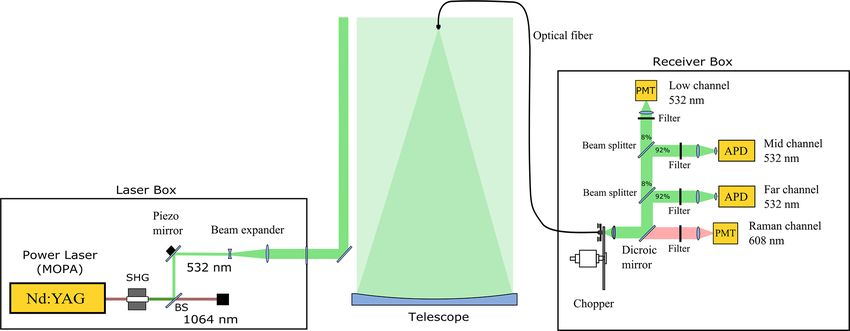
B. Kaifler and N. Kaifler: Compact Rayleigh Autonomous Lidar                                                                          1721

Figure 7. Performance of the conscan system during the measurement on 3 November 2019. (a) Mean scan mirror angles, (b) lidar return
signal integrated between 45 and 55 km altitude, (c) phase and (d) amplitude of the demodulated conscan signal, and (e) goodness of the fit.

stable throughout the lidar measurement. Note that while the            the finite exposure time, the camera integrates the beam pro-
lidar return signal was impacted by broken clouds during                file along a certain height range. If a cloud drifts through
the first hour, conscan allowed robust beam tracking as in-             the beam within this height range, the image will be dom-
dicated by the peaks in the lidar return signal reaching values         inated by the strong Mie scattering. If that happens at the
of ∼ 8 × 10⁴ , which is approximately the same value as later           bottom (top) of the height range, camera-based autoguiding
when the clouds disappeared.                                            optimizes the beam overlap for low (high) altitudes in bistatic
   Panels c–e of Fig. 7 show the phase, amplitude, and χ 2              lidar configurations. The use of conscan avoids that problem.
value determined from the fits to the conscan signal. The χ 2
value is used as an indicator of the quality of the conscan sig-        2.3.2    Adaptive detector gating
nal. Note that we do not normalize the conscan signal prior
to fitting the data, and hence, the average χ 2 value is about          As one of the goals of CORAL is to obtain measurements as
20 instead of unity even for signals with a large signal-to-            often as possible, it was clear from the very beginning that
noise ratio. A large χ 2 value – we use 300 as threshold –              CORAL would also operate in marginal weather, e.g., haze
indicates that the conscan signal could not be properly de-             and variable cloud cover. Although these conditions diminish
modulated. In this case, the conscan cycle is aborted, and the          the lidar return signal, being a Rayleigh lidar, CORAL has
beam pointing is not updated. In cloudy conditions, as many             still enough power margin to produce scientifically usable
as 9 out of 10 conscans may fail in that way, but the succeed-          measurements in the stratosphere and lower mesosphere.
ing conscans are still sufficient for beam tracking as thermal          However, the weaker signal requires that the gating of the
drifts happen on relatively long time scales. If more than 10           APDs and the opening of the chopper have to be adjusted
successive conscans fail, subsequent intervals are marked in            to lower altitudes to make use of the full dynamic range of
the raw data files of the lidar as potentially having incomplete        the detectors and allow for assembly of the individually re-
beam overlap and are discarded in the temperature retrieval.            trieved temperature profiles into a single continuous profile
Moreover, beam pointing increments and conscan parame-                  (see Fig. 8).
ters are stored in raw data files for offline analysis. As evident         Our implementation of adaptive controls for detector gat-
from Fig. 7e, only a few conscan measurements exceed the                ing is rather simple. The data acquisition software integrates
threshold of χ 2 > 300 even though the lidar return signal was          photon counts for 2 s intervals and calculates peak count rates
strongly impacted by clouds in the period 04:00–05:00 UTC.              for each detector channel. If the peak count rate is outside
The larger uncertainties in that period are also reflected in the       a predefined dead band, the delay of the gating signal for
larger amplitude estimates (Fig. 7d).                                   the respective channel is increased by 3 µs if the count rate
   It is important to note that conscan always evaluates the li-        is high or decreased by 3 µs if the count rate is low. The
dar signal within a constant altitude range in the stratosphere.        change is equivalent to an increase or decrease in the gat-
This is in particular beneficial for bistatic lidars in which in        ing altitude in steps of 450 m. We use different dead bands
an autoguiding setup (Innis et al., 2007), the camera images            [4.0, 5.5 MHz], [5.5, 6.5 MHz], and [8.0, 9.0 MHz] for the far
the laser beam at an angle in the lower troposphere as scat-            channel, mid-channel, and low channel, respectively. The
tering in the stratosphere is too weak for imaging. Due to              lowest peak count rates are reserved for the far channel in
                                                                        order to limit thermal heating of the APD and thus reduce

https://doi.org/10.5194/amt-14-1715-2021                                                   Atmos. Meas. Tech., 14, 1715–1732, 2021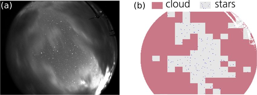
1722                                                            B. Kaifler and N. Kaifler: Compact Rayleigh Autonomous Lidar

Figure 8. (a) Photon count profiles acquired on 3 November 2019 between 05:20 and 05:50 UTC and binned to 100 m vertical resolution,
and (b) retrieved temperature profiles at 900 m vertical resolution. The shaded areas indicate the temperature uncertainties as determined by
the retrieval (see Sect. 4). For comparison, the corresponding SABER profile (acquired at 525 km mean distance to the west of CORAL at
05:38 UTC) and 06:00 UTC ECMWF integrated forecasting system (IFS) profile (0.125◦ resolution, grid point 53.75◦ S, 67.75◦ W, 3.9 km
distance to CORAL) are also shown as gray lines and black dashed lines, respectively.

nonlinear effects that may strongly affect retrieved temper-             FPGA controlling the laser. In case the software crashes, the
atures at upper mesospheric altitudes where the lidar return             kill timer runs out and the laser is automatically shut down
signal is low. Nonlinear effects at low count rates are of less          after 3 s.
importance in the case of the other channels because, at the
top of the profiles, there is sufficient overlap with tempera-           2.4   Container
ture profiles retrieved from other channels.
                                                                         The CORAL container provides all the necessary infrastruc-
2.3.3   Air traffic safety                                               ture for the operation of the CORAL lidar instrument. It has
                                                                         two large doors, one in the front providing access to the air-
Eye safety is an important consideration for an automatic li-            conditioned compartment and one in the back for servicing
dar system. The laser beam emitted by CORAL can be dan-                  the telescope (see Fig. 9). Two smaller hatches equipped with
gerous for eyesight even at altitudes of aircraft if one looks           actuators serve as inlet and outlet for the air needed by the
into the beam, and measures must be taken to avoid acciden-              chiller. A third motorized hatch of size 0.8 m by 0.8 m is
tal exposure. A common method is to employ a radar to track              located above the telescope (see also Fig. 1). Finally, two
aircraft and automatically block the laser beam or shut down             smaller openings of size 0.4 m by 0.4 m in the roof enable
the laser when an aircraft approaches the lidar station (see             the installation of transparent domes for passive optical in-
e.g., Strawbridge, 2013). At the southern tip of South Amer-             struments. While one dome is usually occupied by a cloud
ica, air traffic is so low that no particular safety measures            monitoring all-sky camera, the other dome is available to
are requested by the authorities in Argentina. We use an au-             guest instruments such as the Advanced Mesospheric Tem-
tomatic dependent surveillance-broadcast (ADS-B) receiver                perature Mapper (Pautet et al., 2014; Reichert et al., 2019).
for receiving positional data of nearby aircraft. This infor-            The domes can be removed and covers installed to seal the
mation is used by the lidar computers to automatically shut              openings for shipment of the container. A weather station
down the laser when the aircraft enters a circle of 800 m ra-            measuring wind speed, temperature, humidity, and precipi-
dius centered at the location of CORAL, and measurements                 tation completes the external additions.
are resumed when the aircraft has exited the circle. However,               The layout of the interior is sketched in Fig. 9b. The larger
due to the low air traffic and CORAL being located close to              of the two compartments is insulated and air conditioned to
the local airport but outside the flight corridors, within the 3         22±2 ◦ C, whereas the smaller telescope compartment is only
years of operation, no single aircraft was detected within the           equipped with low-power electrical heaters to raise its tem-
critical zone. At other sites in Europe, we employed a com-              perature slightly above the ambient temperature in order to
bination of an ADS-B receiver and a camera-based setup for               reduce the humidity when the lidar is not in operation and
tracking position lights of aircraft. Because CORAL oper-                the telescope hatch closed. The chiller, which is mounted be-
ates only in darkness, the bright position lights result in a            low the ceiling, provides cold glycol with a cooling capacity
good signal-to-noise ratio in the camera images and can be               of 2.4 kW and is used for both secondary cooling of the laser
easily tracked using motion detection algorithms. For protec-            and air conditioning. All of the lidar hardware with the ex-
tion against software crashes, a kill timer, reset by the ADS-B          ception of the telescope is installed in the laser rack below
decoder and optical tracker software, is implemented in the              the chiller. The space between the two boxes marked with

Atmos. Meas. Tech., 14, 1715–1732, 2021                                                    https://doi.org/10.5194/amt-14-1715-2021
B. Kaifler and N. Kaifler: Compact Rayleigh Autonomous Lidar 1723
Figure 9. (a) The CORAL container at the Sodankylä Geophysical Observatory, Finland, with access door (1), optical dome for passive
instruments (2), optical dome for all-sky cloud camera (3), telescope hatch (4), and weather station (5). (b) Layout of the interior with the
water chiller (A) (no air ducts shown), lidar rack (B), telescope (C), space for passive optical instruments (D), motorized chiller hatches (E),
and access doors (F). Picture by B. Kaifler.
“D” in Fig. 9b is normally kept empty and can be used by a is always in a consistent and safe state. There are FPRs deal-
person for servicing the lidar or manual on-site control of the ing with technical faults, as well as, in the view of CORAL,
lidar. dangerous environmental conditions. For example, an FPR
prevents the opening of the telescope hatch if the wind speed
2.4.1 Control as measured by the weather station exceeds a certain thresh-
old, and another FPR is responsible for shutting down the
Control of the container systems, such as heatings, hatch ac- laser and closing of the telescope hatch when precipitation is
tuators, fans, and chiller, is exercised by two ATMEGA644 detected. The implementation of the most critical FPRs at the
8-bit microcontroller units on custom designed electronics MDM level represents a safeguard against adverse effects of
boards. The microcontroller units serve as multiplexers and software errors. Because the software running on the MDMs
demultiplexers (MDMs) by providing discrete signals to re- is less than 3000 lines in total and does not rely on an inter-
lays supplying power to the various subsystems and reading calated operating system, the probability of a software error
data from the weather station, as well as other internal sen- causing a fatal crash or deadlock is much lower than is the
sors, e.g., level sensors and temperature sensors in the glycol case for the application software running on COCON with its
tank of the chiller. Aggregated sensor and status data are sent hundreds of thousands of lines. In that we cannot guarantee
to, as well as commands received from, a high-level con- that the high-level application software is free of errors, we
tainer control computer (COCON) via serial RS-232 links. have to assume that it fails at some point, and hence, with no
Whereas a single-task program with a global event loop runs operator in the loop to intervene, the MDMs must be capable
on the bare hardware of each MDM, COCON is a standard on their own of maintaining the safety and a consistent state
x86-compatible computer running the Linux operating sys- of the CORAL system to prevent fatal outcomes such as leav-
tem and application software written in C/C++. The MDMs ing the hatch open in a rain shower. Following this require-
and COCON normally run in tandem. For example, COCON ment, most FPRs trigger a routine called “safe mode” which
would send a high-level command to switch the chiller on to shuts down the lidar, disables the chiller, closes hatches, and
MDM #1. The MDM decodes the command and translates it reconfigures the heating and ventilation system. It is then up
into a set of low-level instructions for immediate or deferred to the application software running on COCON to recover
execution: commanding the actuators to open the hatches for from the fault that caused the safe mode. Following the ex-
air cooling, wait until the hatches are fully open, close the re- ample with high wind speed, the application software moni-
lay to supply power to the chiller. At the same time, a steady tors data coming from the weather station and, after the wind
stream of sensor data is flowing from the MDM back to CO- has sufficiently abated, restarts the lidar operation.
CON containing, e.g., angle measurements of the hatches and Another more severe example is power failure. All critical
the coolant temperatures. computers, sensor busses and actuators are powered off an
In addition to the multiplexing and demultiplexing func- uninterruptible power supply (UPS). The only exception is
tionality, the software running on the MDMs also includes a MDM #2 which, for reasons of redundancy, is directly con-
basic set of fault protection routines (FPRs). The sole pur- nected to the main power supply. In the event of a power fail-
pose of these FPRs is to guarantee that the CORAL system
https://doi.org/10.5194/amt-14-1715-2021 Atmos. Meas. Tech., 14, 1715–1732, 20211724 B. Kaifler and N. Kaifler: Compact Rayleigh Autonomous Lidar
ure, MDM #2 thus shuts down. Since both MDMs are con- 3.2 Data sources and decision-making
stantly monitoring each other by sending heart beat signals,
MDM #1 detects power failures as an absence of the MDM The decision-making process behind the autonomous capa-
#2 heart beat signal and triggers the corresponding FPR. On bility of CORAL is implemented in a program called auto-
a higher level, the application software running on COCON control. Autocontrol is a rule-based system that seeks an-
also monitors the state of the UPS and has access to addi- swers to questions such as the following. Is it cloudy? Is
tional information such as the battery charging level. While the cloud layer solid (no lidar observations possible) or bro-
the FPR on MDM #1 triggers the closing of all hatches in the ken clouds (lidar observation possible but signal degraded)?
event of a power failure, the application software may shut What is the probability for rain within the next hour? The in-
down the computers if the charging level becomes too low. dividual answers are then combined in logical connections to
The computers boot up automatically after power is restored. arrive at the yes/no decision to start or stop the lidar.
In order for autocontrol to find answers, we have to feed
it with data. The current implementation uses five main data
3 Autonomous lidar operation sources: the solar elevation angle, the local weather station,
the cloud monitoring camera, ECMWF integrated forecast-
3.1 Software architecture
ing system (IFS) data, and lidar data if the lidar instrument is
The three key ingredients that make autonomous lidar op- already running. The solar elevation angle is determined by
eration possible are (i) the ability to control every aspect the fixed location of the instrument and the local time (Mon-
of the lidar instrument and container subsystems by means tenbruck and Pfleger, 2013). Because CORAL can operate
of a computer program, (ii) the availability of robust data in darkness only, we use the elevation angle to restrict op-
based on which the decision can be made whether lidar op- eration times to periods when the solar elevation is below
eration is currently feasible, and (iii) the implementation of −7◦ . The weather station is used for monitoring precipita-
this decision-making logic. tion and wind speed. A rain signal or the wind speed ex-
The first is a pure technical aspect which we realized by ceeding a threshold prevents the automatic start of the lidar
implementing a message-based data exchange system on top or, in cases when the lidar is already running, triggers an
of a client–server architecture. The functionality of each sub- immediate shutdown. The cloud monitoring camera is a 1.3
system such as lidar data acquisition, laser, and autocontrol megapixel monochrome charge-coupled device (CCD) cam-
– this part contains the decision-making logic – is imple- era (Basler acA1300-30gm) combined with a 1.4 mm f/1.4
mented in separate computer programs that communicate via fishy eye lens (Fujinon FE185C046HA-1). We use a blob
the message system. For example, autocontrol inquires from finding algorithm to detect stars in long exposures, and stars
the data acquisition about the strength of the lidar return sig- are counted within a region extending from zenith to 50◦
nal, and the data acquisition reports the numbers back to au- off-zenith. The star count is used by autocontrol to assess
tocontrol by replying to that message. In another example, whether the sky is clear (large number of detected stars) or
the autotrack program which tracks the laser beam requests cloudy (low number of detected stars). An example image
photon count data from the data acquisition, processes the along with a map containing positions of detected stars is
data, and sends a message to the lidar electronics to update shown in Fig. 10.
the beam pointing. Short messages that may contain only Relying solely on star images to discern clear sky has the
few parameters or data values are implemented using the disadvantage that this information is only available when the
Standard Commands for Programmable Instruments (SCPI) sky is sufficiently dark for stars to be seen (solar elevation
protocol (SCPI, 1999), while larger data sets are sent as bi- angle < −11◦ ). However, in order to facilitate early starts of
nary blobs preceded by a unique identifier. SCPI is a human the lidar and thus maximize the run time, we need informa-
readable protocol. For example, the command laser:shutter 1 tion on sky condition already at twilight. This information
prompts the laser to open its shutter. All aspects of the lidar is retrieved from ECMWF forecast data in the form of the
system can be controlled without the need for a graphical parameters total cloud cover and total precipitation for the
user interface by typing SCPI commands in a terminal. This grid point nearest to the location of CORAL. Lidar start is
simplified the testing and debugging of the software a lot allowed if the cloud fraction is below 0.5 and accumulated
given that in total more than 1000 commands are currently precipitation within the next 2 h is below 0.1 mm.
implemented in the lidar software, the majority representing After the lidar is up and running, the strength of the li-
configuration parameters. SCPI commands also can be col- dar return signal is used as additional information for the
lected in text files that are loaded and sent automatically at assessment of clouds. If the signal strength is greater than
the startup of a program. 70 % of the expected maximum signal, the sky is classified
as clear and lidar operation is allowed to continue even in
cases of ECMWF forecasting precipitation. The reasoning
behind this rule is that the predicted occurrence of rain show-
ers is often off by more than 1 h and the effect of rain showers
Atmos. Meas. Tech., 14, 1715–1732, 2021 https://doi.org/10.5194/amt-14-1715-2021B. Kaifler and N. Kaifler: Compact Rayleigh Autonomous Lidar 1725
Figure 10. (a) Image acquired by the cloud monitoring camera and (b) detected stars. Image by N. Kaifler.
can be very localized in the surroundings and not necessarily below −7◦ , which happens at 22:15 UTC. Then autocontrol
at the precise location of CORAL. By allowing the lidar to verifies that the precipitation forecasted by ECMWF for the
continue observations when the signal is good prevents un- next 2 h is below 0.1 mm (Fig. 11c), the measured wind speed
necessary shutdowns. The idea here is that precipitation is is below the threshold of 110 (equivalent to approximately
preceded by a cloud layer that can be indirectly detected by 15 m s−1 ), and the rain sensor does not detect any rain. No
the lidar as drop in the lidar return signal strength. Follow- conditions are violated and autocontrol initiates the starting
ing that, the lidar is stopped in cases when the signal drops sequence of the instrument. Data collection begins approxi-
below 70 % and ECMWF forecasts > 0.1 mm of precipita- mately 5 min later with photon count rates averaged between
tion. But even if no precipitation is forecasted, the clouds 50 and 60 km altitude reaching about 340 kHz (Fig. 11f).
may thicken enough that continuing the lidar operation is At 23:08 UTC, a fault protection routine within autocontrol
not worthwhile anymore because of the low lidar signal. For detects the crash of the experimental data acquisition soft-
this case we implemented a 15 min count down timer that ware we were testing at that time and triggered a shutdown
is started when the lidar signal drops below 20 %, and the of the instrument. The crash is evident in the photon count
lidar is stopped when the counter reaches zero. In order to rate being constant, indicating that a key metric of the data
let the lidar continue its observations in broken clouds, the acquisition software is not updated any more. At the same
counter is reset to 15 min every time the signal increases be- time, the ECMWF precipitation forecast exceeds the thresh-
yond the 20 % threshold. A final rule introduces a mandatory old of 0.1 mm and thus prevents autocontrol from restarting
wait period of 30 min following a shutdown triggered by low the instrument until 2 h later, though the sky remains mostly
signal. This rule was implemented after we discovered that cloudless as indicated by the high number of detected stars
light scattered off dust particles on the optical dome cover- (Fig. 11e). Finally, at 02:15 UTC, a simultaneous decrease
ing the all-sky camera is sometimes misinterpreted as stars. in photon count rate and number of detected stars suggest
In some cases, the high number of artificial stars leads to the appearance of clouds. Lidar measurements continue un-
a constant startup–shutdown cycle even though the sky was til about 30 min later when the wind speed crosses briefly
overcast and no meaningful lidar observations could be ob- the threshold and autocontrol triggers another shutdown of
tained. The implementation of the wait period reduces the the instrument. The number of detected stars remains zero
number of start attempts to a level that does not cause exces- while a short rain event is detected at 03:20 UTC. Although
sive wear. the star count increases shortly after, the startup of the li-
The current state of the lidar is tracked in a global state dar is blocked by the 30 min wait period following a shut-
machine where violations of the rules described above trigger down. This is a safety mechanism as it is not clear whether
state changes. Rules are evaluated once per second, though the nonzero star count is due to real stars being detected
data tables may be updated at different intervals depending (cloudless sky) or due to light scattered off rain droplets on
on the data source and how often new data become available. the camera dome. Half an hour later, the star count goes to
zero, indicating clouds. When the star count increases again
3.3 Example at about 04:00 UTC, autocontrol initiates the startup of the
instrument. Data collection continues until 4 h later when the
Figure 11 shows the data used by autocontrol to make photon count rate and the star count reach low values. At
start/stop decisions on the night of 23–24 August 2020. The 09:00 UTC, the sky clears up again, and autocontrol restarts
ECMWF cloud fraction (Fig. 11b) is below 0.4 during the the lidar, which then runs until the solar elevation angle in-
whole night, indicating to autocontrol that no significant creases beyond −7◦ .
cloudy periods are to be expected. The startup of the lidar
is blocked until the solar elevation angle (Fig. 11a) decreases
https://doi.org/10.5194/amt-14-1715-2021 Atmos. Meas. Tech., 14, 1715–1732, 20211726 B. Kaifler and N. Kaifler: Compact Rayleigh Autonomous Lidar
.
Figure 11. (a–f) Example data used by autocontrol to make start/stop decisions and (g) retrieved temperature profiles. Red areas mark periods
with violated conditions, and beige areas indicate actual instrument run times.
The example shown in Fig. 11 is representative of an by integrating relative number densities from top to bottom.
observation that would have kept a human operator busy One complication arises from the requirement to start the in-
throughout the night. Instead, the CORAL instrument took tegration at infinity in which the density is zero. Since this is
all decisions on its own and even recovered from a software impractical because of the large noise in lidar measurements
crash without human intervention. About 2 h of data were at very high altitudes, the integration is instead split into two
lost due to the crash, as high photon count rates normally parts. Above a certain reference altitude z0 , the integration
take precedence over the ECMWF precipitation forecast and, is assumed to evaluate to a reference temperature T0 that is
in this case, would have allowed the observation to continue. then used to initialize or “seed” the integration of the sec-
ond part starting at z0 . Typically, z0 is chosen as the upper
boundary of the lidar return profile where the signal is still
4 Temperature retrieval reliable, and the corresponding T0 is taken from other mea-
surements or models (e.g Duck et al., 2001; Alexander et al.,
Our implementation of the temperature retrieval is based 2011). The condition “no aerosols present” can be relaxed
on the integration method developed by Hauchecorne and if inelastic (Raman) scattering, e.g., for nitrogen molecules,
Chanin (1980). In the absence of aerosols and absorption by is used instead of the elastic scattering to derive profiles of
trace gases such as ozone and after taking into account the relative number density.
geometric factor z−2 stemming from the formation of spher- In our implementation of the retrieval, the basic prepara-
ical waves of the scattered light, the lidar return signal can be tory steps prior to the integration are binning the photon
assumed as proportional to the Rayleigh backscatter of the count data to a 100 m vertical grid and a desired temporal
atmosphere (e.g., Leblanc et al., 1998). Because Rayleigh resolution, the correction of detector dead-time effects, sub-
scattering is directly proportional to the number density of traction of the background which is estimated from photon
air, the Rayleigh backscatter profile equates to a profile of count profiles between 130 and 200 km altitude, correction of
relative number density. In the retrieval, the atmosphere is the two-way Rayleigh extinction, range-correction by mul-
split up in discrete layers, and the relative number density is tiplication with the range squared, and vertical smoothing
evaluated at these layers from layer averages of the Rayleigh to 900 m effective vertical resolution to improve the signal-
backscatter profile assuming that the number density varies to-noise ratio (SNR). After performing these steps, tempera-
exponentially across layers. Using the ideal gas law and as- tures are computed by integration of the profiles of relative
suming hydrostatic equilibrium, temperatures are calculated density. This process is repeated independently for each de-
Atmos. Meas. Tech., 14, 1715–1732, 2021 https://doi.org/10.5194/amt-14-1715-2021B. Kaifler and N. Kaifler: Compact Rayleigh Autonomous Lidar 1727
tector channel. The question is now, where do we get the seed eration, the temporal resolution is increased to 30 min using
value from? We start off with the nightly mean profile of the seed values taken from the 60 min profiles. Iteration by iter-
far-channel which we seed with an approximately co-located ation, a pyramid with ever increasing resolution is built up
SABER (Sounding of the Atmosphere using Broadband until the desired resolution is reached and at which point the
Emission Radiometry instrument on the Thermosphere Iono- algorithm stops. In Fig. 12b and c, we show an example to
sphere Mesosphere Energetics Dynamics, TIMED, satellite) demonstrate the effect of increasing resolution on tempera-
profile at typical altitudes of 98–108 km. As coincidence cri- ture profiles. Where the 120 min retrieval reveals only large-
teria, we chose a maximum horizontal distance of 1000 km scale structures, in this case signatures of an internal gravity
between the mean location of the satellite measurement and wave with a period of ∼ 6 h and 22 km vertical wavelength,
the location of CORAL. Because the density profiles from the high-resolution retrieval (Fig. 12c) yields a multitude of
the lower channels overlap with an upper channel, we can fine details including smaller-scale waves. The semidiurnal
then seed the retrieval of the mid-channel temperature pro- tide with a period of 12 h may also be present in Fig. 12b
file with a temperature value from the far-channel. In a simi- and c but is overshadowed by internal gravity waves with
lar way, both the low channel and Raman channel are seeded much larger amplitudes. Eckermann et al. (2018) show mea-
with a value taken from the mid-channel temperature profile. surements of tides acquired with a predecessor instrument of
The altitude where the integration starts√and the seed value CORAL above New Zealand with peak amplitudes of ∼ 6 K
is taken is determined by the SNR N ∗ / N, where N is the at 85–90 km altitude (their Fig. 12).
number of detected photons per 100 m bin and N ∗ the de- The implementation of our retrieval also allows us to in-
sired signal (background subtracted). We define the seed al- crease the vertical resolution to, e.g., 500 and 300 m in re-
titude as the maximum altitude with SNR > 4 (far-channel) gions where the SNR is sufficient. A high vertical resolu-
and SNR > 15 (all other channels). The criterion SNR > 4 at tion is especially important for retrieving accurately the large
100 m bin width translates to a relative uncertainty in pseudo- vertical temperature gradients induced by large-amplitude
density of 8.3 % in the case of the default resolution of 900 m waves that are on the verge of becoming convectively un-
and 6.5 % for 1500 m resolution. For reference, a threshold of stable. Due to the SNR required, generally, these very high-
10 % was used by Alexander et al. (2011). resolution retrievals are limited to altitudes of 30–70 km.
The individual temperature profiles are then merged A common way for estimating the uncertainty of retrieved
into a single continuous profile. In order to guarantee a temperatures T (z) is computing the error propagation in the
smooth transition from one profile to another, we compute a hydrostatic integration of the density profiles. Here, the as-
weighted average in the overlapping region using the weight- sumed errors √ of the density profiles are the photon count
ing function w (z) = 0.5 + 0.5 cos (π (z − zt ) /1z) within the uncertainties N (z) scaled accordingly. In our implemen-
transition region starting at altitude zt and vertical extent tation, we use a different approach. Starting
√ with the photon
1z. The bottom of the upper of the two profiles is typically count profile N (z) and its uncertainty N (z), we perform a
chosen as zt and 1z = 2 km. Figure 8 shows an example set of 200 Monte Carlo experiments for each profile. In these
of individually retrieved temperature profiles and overlap- experiments, the number
√ of detected photons per bin N is re-
ping regions. Note the large discrepancy between the Raman placed with N + α N, with α being random numbers drawn
temperature profile (channel 4) and the elastic temperature from a Gaussian distribution with a standard deviation of one
profile (channel 3) at about 20 km altitude, which is caused and zero mean. Then we apply the data reduction steps de-
by stratospheric aerosols. We mitigate the impact of strato- scribed above and run the retrieval separately for each of the
spheric aerosols by transitioning to Raman temperatures be- 200 synthetic photon count profiles. In a last step, the final
low 32 km altitude when merging profiles. temperature profile is computed as the mean of all 200 re-
In order to achieve higher temporal resolutions, we im- trieved profiles, and its uncertainty is given by the standard
plemented the iterative approach sketched in Fig. 12a. Af- deviation.
ter retrieving the nightly mean profile seeded with SABER The Monte Carlo method has the big advantage that all
data, we bin the photon count data to overlapping 120 min data reduction steps are included in the assessment of tem-
wide bins that are offset by 30 min. Temperature profiles are perature uncertainties 1T (z) in a completely natural way.
then retrieved from these binned data using seed values taken That also applies to the initial seed temperatures taken from
from the nightly mean profile. This works because the SNR the SABER profile during the first iteration, i.e., retrieval
of the 120 min binned photon count profiles is always lower of the nightly mean profile. Of course, the seed tempera-
(or equal) to the SNR of the nightly mean profile for the ture is also fraught with uncertainty due to true measure-
same altitude. The result of such a coarse temperature re- ment errors but also because the SABER measurements may
trieval is shown in Fig. 12b. Having completed the 120 min have been acquired up to 1000 km away from the location of
retrieval, we bin the photon count data to 60 min resolu- CORAL. In order to include the impact of variations in seed
tion using 15 min offsets from one bin to the next bin and temperature, we generate a set of seed profiles in the form
start the process over again. This time the seed values are Tseed (z) + α1T (z), one for each of the 200 synthetic photon
taken from the 120 min temperature profiles. In the next it- count profiles, with α being again random numbers that are
https://doi.org/10.5194/amt-14-1715-2021 Atmos. Meas. Tech., 14, 1715–1732, 2021You can also read