GO_3D_OBS: the multi-parameter benchmark geomodel for seismic imaging method assessment and next-generation 3D survey design (version 1.0)
←
→
Page content transcription
If your browser does not render page correctly, please read the page content below
Geosci. Model Dev., 14, 1773–1799, 2021
https://doi.org/10.5194/gmd-14-1773-2021
© Author(s) 2021. This work is distributed under
the Creative Commons Attribution 4.0 License.

GO_3D_OBS: the multi-parameter benchmark geomodel for
seismic imaging method assessment and next-generation
3D survey design (version 1.0)
Andrzej Górszczyk1,2 and Stéphane Operto3
1 ISTerre,Univ. Grenoble Alpes, 38000 Grenoble, France
2 Institute
          of Geophysics, Polish Academy of Sciences, ul. Ks. Janusza 64, 01-452 Warsaw, Poland
3 Université Côte d’Azur, Observatoire de la Côte d’Azur, CNRS, IRD, Géoazur, Valbonne, France

Correspondence: Andrzej Górszczyk (agorszczyk@igf.edu.pl)

Received: 16 July 2020 – Discussion started: 6 October 2020
Revised: 15 February 2021 – Accepted: 15 February 2021 – Published: 31 March 2021

Abstract. Detailed reconstruction of deep crustal targets by      benchmark model is intended to help to optimize the de-
seismic methods remains a long-standing challenge. One            sign of next-generation 3D academic surveys – in particular,
key to address this challenge is the joint development of         but not only, long-offset OBS experiments – to mitigate the
new seismic acquisition systems and leading-edge process-         acquisition footprint during high-resolution imaging of the
ing techniques. In marine environments, controlled-source         deep crust.
seismic surveys at a regional scale are typically carried out
with sparse arrays of ocean bottom seismometers (OBSs),
which provide incomplete and down-sampled subsurface il-
lumination. To assess and minimize the acquisition foot-          1   Introduction
print in high-resolution imaging process such as full wave-
form inversion, realistic crustal-scale benchmark models are      To make a step change in our understanding of the geo-
clearly required. The deficiency of such models prompts us to     dynamical processes that shape the earth’s crust, we need
build one and release it freely to the geophysical community.     to improve our ability to build 3D high-resolution multi-
Here, we introduce GO_3D_OBS – a 3D high-resolution ge-           parameter models of geological targets at the regional scale.
omodel representing a subduction zone, inspired by the ge-        This deep target reconstruction is typically beyond the range
ology of the Nankai Trough. The 175 km × 100 km × 30 km           of the streamer-based data acquisition due to the limited
model integrates complex geological structures with a vis-        length of the streamer cable (∼ 6 km). To meet this chal-
coelastic isotropic parameterization. It is defined in the form   lenge, it becomes crucial to design numerical models and
of a uniform Cartesian grid containing ∼33.6e9 degrees of         related synthetic experiments further promoting a new gen-
freedom for a grid interval of 25 m. The size of the model        eration of crustal-scale seismic surveys. Along with the de-
raises significant high-performance computing challenges to       sign of new acquisition settings, a quest for high-resolution
tackle large-scale forward propagation simulations and re-        reconstruction requires us to assess the feasibility of the
lated inverse problems. We describe the workflow designed         leading-edge seismic imaging techniques and develop their
to implement all the model ingredients including 2D struc-        necessary adaptations to the new acquisition specifications.
tural segments, their projection into the third dimension,        In the context of this study, by seismic imaging we un-
stochastic components, and physical parameterization. Var-        derstand the broad range of procedures for estimating the
ious wavefield simulations that we present clearly reflect        earth’s rock parameters from seismic data – including travel
in the seismograms the structural complexity of the model         time tomography, migration-based velocity analysis, ray-
and the footprint of different physical approximations. This      based and reverse-time pre-stack depth migration, and full
                                                                  waveform inversion. Among them, velocity reconstruction

Published by Copernicus Publications on behalf of the European Geosciences Union.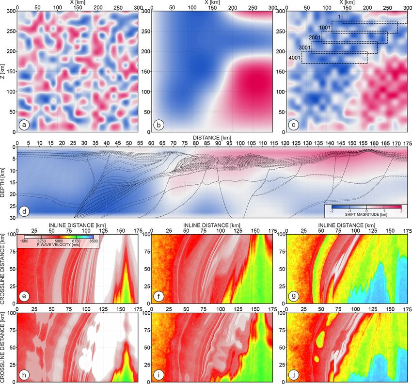
1774                                                                               A. Górszczyk and S. Operto: GO_3D_OBS

methods including first-arrival travel time tomography (FAT)        3D wide-azimuth streamer surveys with a swath of ∼ 1 km
(Zelt and Barton, 1998), reflection tomography (Bishop et al.,      in width and streamers of up to 15 km in length arranged
1985; Farra and Madariaga, 1988), joint refraction and re-          in a single or multi-vessel configuration. The long streamers
flection tomography (Korenaga et al., 2000; Meléndez et al.,        and wide receiver swaths combined with shooting the lines
2015), slope tomography (Billette et al., 1998; Lambaré,            in a race track mode would make the acquisition time of the
2008; Tavakoli F. et al., 2017, 2019; Sambolian et al., 2019),      crustal-scale surveys reasonable (Li et al., 2019) while at the
wavefront tomography (Bauer et al., 2017), finite-frequency         same time increasing the penetration depth of the wavefield.
travel time tomography (Mercerat and Nolet, 2013; Zelt and             For stationary-receiver surveys, coarse 3D passive- or
Chen, 2016), wave equation tomography (Luo and Schuster,            active-source OBS experiments have begun to emerge in
1991; Tong et al., 2014), and full waveform inversion (FWI)         academia (Morgan et al., 2016; Goncharov et al., 2016;
(Tarantola, 1984; Mora, 1988; Pratt et al., 1996) shall be ex-      Heath et al., 2019; Arai et al., 2019). Sparse areal OBS de-
amined against large-scale numerical problems and complex           ployments provide the necessary flexibility to design long-
synthetic datasets generated in an ultra-long-offset configu-       offset acquisition geometries, such that energetic diving
ration. Combining these methods with the up-to-date seismic         waves and post-critical reflections could sample the deepest
acquisition techniques available nowadays should allow for          targeted-structures (lower crust, Moho, upper mantle). While
regional-scale seismic imaging of continental margins at sub-       recent trends in exploration industry show intensive develop-
wavelength spatial resolution (typically few hundred metres)        ment toward seabed acquisitions carried out with large pools
(Morgan et al., 2013).                                              of autonomous nodes (Ni et al., 2019; Blanch et al., 2019),
   During the last decades, a vast majority of deep-crustal         it creates the opportunity to adapt this development to aca-
seismic experiments carried out in academia were performed          demic regional experiments through a relaxation of the ac-
in two dimensions (namely, along profiles), mainly due to           quisition sampling. Indeed, industry-oriented surveys are of-
the financial cost of such experiments and the lack of suit-        ten designed with the aim to apply the entire seismic imaging
able equipments. They often combine a short-spread towed-           workflow to the recorded dataset (namely velocity analysis
streamer acquisition with sparse 4C (four-component) OBS            and migration). For this purpose, large pools of receivers are
(ocean bottom seismometer) deployments. The data recorded           required to fulfil sampling criteria for high-frequency migra-
by these two types of acquisition conceptually provide com-         tion (Li et al., 2019). This requirement can be relaxed when
plementary information on the subsurface, which is pro-             aiming at the velocity reconstruction only using frequencies
cessed with different imaging techniques (Górszczyk et al.,         lower than 15 Hz (Mei et al., 2019).
2019). Streamer data are used for migration-based imaging              In terms of imaging, processing of streamer data interlaces
of the reflectivity of the uppermost crust, while the OBS data      two tasks under a scale-separation assumption: reconstruc-
are routinely utilized to build smooth P-wave velocity mod-         tion of the reflectivity by depth migration (from ray-based
els of the crust by FAT. However, the rapidly increasing in-        Kirchhoff migration to two-way wave equation reverse-time
accuracy of the migration velocities with depth and the lack        migration, RTM) and velocity model building by reflection or
of aperture coverage provided by streamer acquisition gen-          slope tomography. Stable velocity model building with those
erate poor-quality migrated sections at depths exceeding the        techniques can be performed down to a maximum depth of
streamer length. On the other hand, the low resolution of the       the order of the streamer length. In turns, reflectivity imaging
velocity models built by FAT prevents an in-depth geological        by migration may be performed at greater depths if reliable
interpretation of complex media. Put together, these two pit-       deep velocity information is provided (e.g. from complemen-
falls currently make the joint interpretation of migrated sec-      tary OBS data) and the deep reflection are recorded with an
tions and tomographic velocity models quite illusory. More-         acceptable signal-to-noise ratio. Higher-resolution velocity
over, off-plane wavefield propagation makes the 2D acqui-           models can also be built from streamer data by FWI (Shipp
sition geometry implicitly inaccurate, further increasing the       and Singh, 2002; Qin and Singh, 2017) if the information car-
uncertainty of the resulting images. The need for enhance-          ried out by diving waves is made usable after the re-datuming
ment of this acquisition and processing paradigm is therefore       of the data on the seabed (Gras et al., 2019). As an alternative
obvious.                                                            to classical FWI, a velocity model can be built by reflection
   Regarding streamer acquisition, to date only a few 3D            waveform inversion (RWI), a reformulation of FWI where
academic multi-streamer experiments have been conducted             the reflectivity estimated by least-squares RTM is used as a
(Bangs et al., 2009; Marjanović et al., 2018; Lin et al., 2019).   secondary buried source to update the velocities along the
However, these experiments were performed with a small              reflection paths connecting the reflectors to the sources and
number of streamers and small spread (typically ∼ 6 km).            receivers (Xu et al., 2012; Brossier et al., 2015; Zhou et al.,
The limited width of the receiver swath leads to narrow az-         2015; Wu and Alkhalifah, 2015).
imuth coverage and prevents the survey of a large area with            All these approaches have been designed to deal with
a reasonable acquisition time, while the short length of the        the limited aperture illumination provided by short-spread
streamer limits the maximum depth of investigation as above         streamer acquisition, which generates a null space between
mentioned. In contrast, the oil industry nowadays carries out       the low wavenumbers of the velocity macro-model and the

Geosci. Model Dev., 14, 1773–1799, 2021                                             https://doi.org/10.5194/gmd-14-1773-2021
A. Górszczyk and S. Operto: GO_3D_OBS                                                                                         1775

high wavenumbers of the reflectivity image, hence justifying         difficult to satisfy when the number of propagated wave-
the explicit above-mentioned scale separation during seis-           lengths increases as in the case of ultra-long-offset regional
mic imaging (Claerbout, 1985; Jannane et al., 1989; Neves            surveys (Pratt, 2008). This issue can be addressed by de-
and Singh, 1996). Compared to streamer data, long-offset             veloping kinematically accurate starting velocity models by
OBS data recorded by stationary-receiver surveys contain a           travel time tomography (Górszczyk et al., 2017); by breaking
wider aperture content and richer information about the deep         down FWI into several data-driven multiscale steps accord-
crust and upper mantle. This information can be processed by         ing to frequency, travel time, and offset continuation strate-
travel time tomography and waveform inversion techniques –           gies (Kamei et al., 2013; Górszczyk et al., 2017); by de-
the former providing a kinematically accurate starting model         signing more robust distances in FWI (Warner and Guasch,
for the latter (Kamei et al., 2012; Górszczyk et al., 2017). The     2016; Métivier et al., 2018); or by extending the linear regime
term “long-offset data” refers to seismic data which record          of FWI by the relaxation of the physical constraints (van
diving and refracted waves that undershoot the targeted struc-       Leeuwen and Herrmann, 2013; Aghamiry et al., 2019a). The
tures. Under this condition, the angular illumination of the         final key challenge is related to the computational burden
structure is sufficiently wide to build high-resolution crustal      resulting from wave simulation in huge computational do-
models by FWI. Therefore, FWI should be regarded as the              mains. The only panacea here can be given through a devel-
method of choice for long-offset stationary-receiver data.           opment of efficient, massively parallel modelling, inversion,
   FWI is a brute-force nonlinear waveform matching proce-           and optimization schemes tailored to the high-performance-
dure which allows for building broadband subsurface mod-             computing architecture available nowadays.
els – provided that the structure is illuminated by a vari-             As reviewed above, advanced deep-crustal seismic imag-
ety of waves propagating from the transmission to the re-            ing raises different frontier methodological issues in terms
flection regime (Sirgue and Pratt, 2004). Diving waves, pre-         of acquisition design, inverse problem theory and high-
and post-critical reflections, diffractions, etc., have the poten-   performance computing. Addressing these challenges can be
tial to generate a wide range of scattering from the targeted        done by establishing a geologically meaningful 3D marine
structure and therefore can probe this structure with vari-          regional model amenable to exploring the pros and cons of
ous wavenumber vectors (Fig. 1a). By a broadband model               different acquisition geometries, wave propagation require-
we understand a low-pass-filtered version of the true earth,         ments, and processing techniques. Indeed, most of the ge-
where the local cut-off wavenumbers in each x, y, and z spa-         omodels in the imaging community have been designed to
tial direction are controlled by the local wavelength and the        fit the specifications of the exploration scale (Marmousil
scattering, dip, and azimuth angles sampled by the acquisi-          Versteeg, 1994; SEG/EAGE salt and overthrust, Aminzadeh
tion (Fig. 1b). This means that the resolution obtained with         et al., 1997; 2004 BP salt model, Billette and Brandsberg-
FWI depends not only on the frequency bandwidth of the               Dahl, 2004; SEAM models, Pangman, 2007), while available
data but also on the aperture with which the wave interacts          crustal-scale geomodels are rather smooth or lack well de-
with the heterogeneities to be reconstructed (Operto et al.,         fined structures and are 2D (e.g. 2D CCSS blind-test model,
2015). Fulfilling this wide-angular illumination specification       Hole et al., 2005; Brenders and Pratt, 2007b, a). In contrast
is the first fundamental methodological issue for successful         our proposed geomodel shall incorporate a representative
application of FWI to OBS data. Indeed, this wide-aperture           sample of three-dimensional geological structures detectable
illumination provided by long-offset acquisition is achieved         at the seismic scale (faults, sediment cover, main structural
at the expense of the receiver sampling, whose imprint in            units, and discontinuities) and a multi-parameter physical
the model reconstruction should be assessed. When a lim-             definition of those structures (Wellmann and Caumon, 2018).
ited pool of instruments is available, the down-sampling of          A suitable natural environment to fulfil such specifications
the acquisition is directly mapped into the down-sampling            is provided by subduction zones. Indeed, the complex ge-
of the subsurface wavenumbers, leading to spatial aliasing           ological architecture of these margins warrants the variety
or wraparound in the spatial domain. A second fundamen-              of structures characterized by distinct physical parameters.
tal methodological issue is therefore to mitigate the alias-         Moreover, convergent margins still crystallize in many stud-
ing artefacts by reliable compressive sensing techniques and         ies on the role of structural factors (sea mounts, subduction
sparsity-promoting regularization during FWI (Herrmann,              channel, etc.) and fluids on the rupture process of megath-
2010; Aghamiry et al., 2019b). The third main issue is re-           rust earthquakes (Kodaira et al., 2002). Therefore, capitaliz-
lated to the well-known nonlinearity of the FWI associated           ing on our experiences from the previous imaging studies in
with cycle skipping (e.g. Virieux and Operto, 2009). When            the region of the eastern Nankai Trough (Dessa et al., 2004;
a classical form of the least-squares misfit function is used        Operto et al., 2006; Górszczyk et al., 2017, 2019) and com-
(namely, the least-squares norm of the difference between            bining them with the diverse geological features – typically
the simulated and the recorded data), FWI can remain stuck           interpreted in the convergent margins around the world – we
in a local minimum when the initial model does not allow             aim at building a regional synthetic model of the subduction
one to predict travel times with errors smaller than half a          zone.
period. The cycle-skipping condition is indeed increasingly

https://doi.org/10.5194/gmd-14-1773-2021                                               Geosci. Model Dev., 14, 1773–1799, 2021
1776 A. Górszczyk and S. Operto: GO_3D_OBS
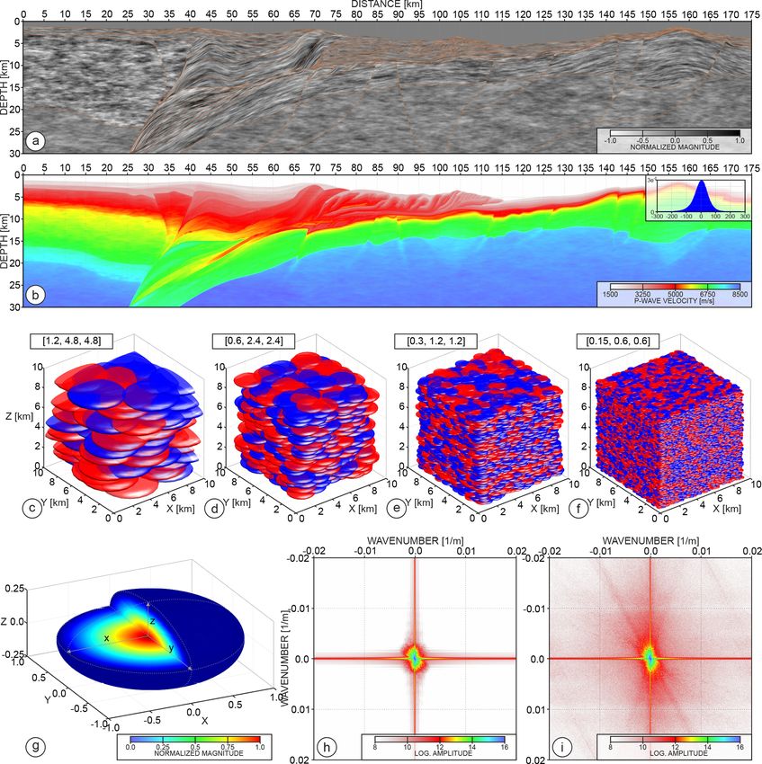
Figure 1. (a) Sketch of the single source/receiver (S/R) acquisition and the 3D wavenumber vector k mapped by FWI at the scattering point
P. (b) Zoom on (a). Local wavenumber vector k is a sum of the k s and k r vectors associated with the ray paths emerging from the source S
and receiver R creating the scattering angle θ at the scattering point P. Dip and azimuth of the wavenumber vector k are defined by the φ and
ϕ angles. The modulus of k is given by (λ/2) cos(θ/2), where λ denotes the local wavelength (Miller et al., 1987; Wu and Toksöz, 1987).
The range of k mapped at each point P by the acquisition gives the resolution with which the subsurface is reconstructed by FWI.
The proposed geomodel is intended to serve as an exper- fore, away from the challenges related to the reconstruction
imental setting for various imaging approaches with a spe- of the geologically complex setting, the model imposes a sig-
cial emphasize on multi-parameter waveform inversion tech- nificant computational burden in terms of seismic wavefield
niques. For this purpose, the size of geological features we modelling. The large size of the computing domain can fur-
introduce shall be detectable by seismic waves and span tens ther contribute to the development of efficient forward or in-
of kilometres (major structural units building mantle, crust, verse problem solvers (time- and/or frequency-domain wave-
volcanic ridges, etc.) to tens of metres – namely to the order field modelling, eikonal, and ray-tracing solvers, etc.) dedi-
of the smallest seismic wavelengths (sedimentary cover, sub- cated to crustal-scale imaging.
ducting channel, thrusts, and faults, etc.). The structural com- This article is organized as follows. We start with the de-
plexity of the model is complemented by a broad range of scription of the geological units, which build the 2D curvi-
physical parameters. Our approach incorporates determinis- linear structural skeleton of the model. Then, we review how
tic, stochastic and empirical components at various stages of we project the 2D initial structure into the third dimension
the model building. The deterministic components cover the and how we introduce the viscoelastic properties in each
shape of the main geological units, as well as their projection structural unit. Third, we describe the implementation of the
into the third dimension. The stochastic components include stochastic components designed to introduce more structural
small-scale perturbations and random structure warping – in- heterogeneity. Finally, we present some simulations of OBS
troducing further spatial variation (Holliger et al., 1993; Goff data in the 3D model with the finite-difference and spectral-
and Holliger, 2003; Hale, 2013). The empirical components element methods, and we summarize the article with a dis-
combine the physical parameterization of the model – Vp , Vs , cussion and conclusion.
ρ (density), Qp , Qs – namely the magnitude and relations be-
tween the subsequent parameters (Brocher, 2005; Wiggens
et al., 1978; Zhang and Stewart, 2008). Such a combina- 2 Model building
tion of structural and parametric variability is reflected by
the anatomy of the seismic wavefield, making it suitable to In the following sections we present, step by step, the work-
benchmark different imaging approaches. We obtain the 3D flow that was designed to create the seismologically repre-
cube through the projection of the initial 2D inline profile sentative model of the subduction zone. The whole procedure
towards the strike direction of subduction, leading to real- was implemented in a MATLAB environment.
istic changes in the geological structure along the crossline
2.1 Geological features
extension of the model. The dimension of the final model
equals 175 km×100 km×30 km leading to ∼ 33.6e9 degrees The overall geological setup of our model is mainly (but
of freedom in a Cartesian grid with a 25 m grid step. There- not only) inspired by the features interpreted in the Nankai
Geosci. Model Dev., 14, 1773–1799, 2021 https://doi.org/10.5194/gmd-14-1773-2021
A. Górszczyk and S. Operto: GO_3D_OBS                                                                                       1777

Trough area. However, these structures can also be found           tinental part, two blue dashed lines mark major boundaries
in different convergent margins around the world combined          creating large flower-like structures, which can be typically
in various configurations. Therefore, our model is not in-         found around strike slip faults zones (Huang and Liu, 2017;
tended to replicate a particular subduction zone and its re-       Ben-Zion and Sammis, 2003; Tsuji et al., 2014). Each of
lated geology for geodynamic studies of the targeted region.       those boundaries can also be further used to implement fluid
On the contrary, it was designed to comprise broad range of        paths or damage zones.
features one may encounter in these tectonic environments.            On top of the oceanic crust, we place two layers of sub-
Such a quantitative subsurface description should challenge        ducting sediments (grey dashed and solid lines in Fig. 2a).
performances of high-resolution crustal-scale imaging from         They extend starting from the subducting channel up to the
the complex waveforms generated in this model.                     right edge of the model. In general, the lower layer is thicker
   The skeleton of the initial 2D model is presented in Fig. 2a.   and overlays directly the top of the oceanic crust covering its
It is designed as a cross section aligned with the direction       thrusts and faults. The upper layer is thinner, whereas its up-
of subduction and consists of 46 geological units. These           per limit delineates the decollement in our model. To provide
units are defined by means of the interfaces creating inde-        more complexity, we introduce a small duplexing structure
pendent polygons and obtained in the following three steps.        within those two layers (between 65 and 85 km in Fig. 2a)
First, we pick the spatial position of the nodes in the cross      similarly to the decollement model presented by Kameda
section (see dots in Fig. 2a). Second, we interpolate piece-       et al. (2017), Hashimoto and Kimura (1999), and Collot et al.
wise cubic Hermite polynomials through a subset of nodes           (2011).
to build a boundary (or interface) between the geological             Just between the edge of the continental crust and the
units. Such boundaries represent either lithostratigraphic dis-    subducting slab, we add a stack of relatively thin sheets
continuities or tectonic features like faults. They can connect    corresponding to progressively underplated material (dashed
and/or intersect with each other to create closed regions in the   black lines in Fig. 2a). Typically these kinds of structures
(x, z) plane representing separate geological units. We refer      occur when sediments, which move down on top of the
to these closed regions as polygons. With such an approach,        subducting oceanic crust, create a duplex system and are
we can modify the shape of existing features or add new ones       further added to the accretionary wedge (Angiboust et al.,
to the initial structure.                                          2014, 2016; Menant et al., 2018; Agard et al., 2018; Ducea
   To create an overall skeleton of the model, we start from       and Chapman, 2018). Including these relatively fine-scale
the interfaces that shape the mantle and the crust. In Fig. 2a,    structures in the deep part of the model will significantly af-
the top of the oceanic or continental crust and mantle are         fect wavefield propagation.
marked by solid red and green lines respectively. The geom-           The accretionary wedge consists of two parts. The land-
etry of the subducting slab is inferred from previous stud-        ward part is formed by large deformed stacked thrusts sheets
ies in the Tokai area. The oceanic crust exhibits variabil-        (solid blue lines in Fig. 2a) corresponding to the old ac-
ity of thickness and local bending consistently with what is       cretionary prism, which extends seawards into large out-of-
proposed by geological studies in the same region (Kodaira         sequence thrusts acting as a backstop now. Similar inner-
et al., 2003; Le Pichon et al., 1996; Lallemand et al., 1992;      wedge structures can be found in various subduction zones
Górszczyk et al., 2019) and addressed as an effect of subduct-     (Dessa et al., 2004; Raimbourg et al., 2014; Shiraishi et al.,
ing volcanic ridges and sea mounts. On the right flank of the      2019; Collot et al., 2008; Cawood et al., 2009; Contreras-
model (starting at 140 km of model distance), we introduce a       Reyes et al., 2010) and can also be modelled with analogue
large volcanic ridge indicated by the uplift of the bathymetry     sand-box experiments (Gutscher et al., 1998, 1996). The
and the significant thickening of the oceanic crust. A similar     outer-wedge (red shaded polygon in Fig. 2a) contains the
ridge (Zenisu Ridge) really exists in the eastern part of the      sedimentary prism adapted from Kington and Tobin (2011)
Nankai Trough. It currently approaches the subduction zone         and Kington (2012) (Fig. 2b). It is built from different types
and simultaneously undergoes the thrusting process (Lalle-         of sediments, which underwent deformation and created a
mant et al., 1989).                                                sequence of thrusts interpreted within the Kumano Basin.
   In the next step, we cut the subducting oceanic crust and       The complexly shaped, small-scale, steeply dipping struc-
mantle by series of interfaces (blue dashed lines in Fig. 2a)      tures will impose a challenge for seismic imaging. In our im-
to subdivide them into several polygons. These interfaces al-      plementation the prism from Fig. 2b is managed as a single
low us to project each of the defined block independently in       block associated with the respective red shaded polygon in
the third dimension (see next Sect. 2.2). They are also de-        Fig. 2a. Depending on the changes in the shape of this poly-
signed to implement tectonic discontinuities in the oceanic        gon during the projection step, we re-sample the prism from
crust and upper mantle. Such discontinuities acting as faults      Fig. 2b such that it conforms to the shape of the polygon.
and thrusts or creating horst-graben structures are well docu-        Finally, the frontal prism is fed by the layers of incom-
mented in subduction zones (Tsuji et al., 2013; Ranero et al.,     ing sediments (black lines in Fig. 2a) – relatively thick in
2005; Azuma et al., 2017; Boston et al., 2014; Vannucchi           the area of the trench and thin over the volcanic ridge. These
et al., 2012; von Huene et al., 2004). At the edge of the con-     sedimentary layers are associated with those interpreted in

https://doi.org/10.5194/gmd-14-1773-2021                                             Geosci. Model Dev., 14, 1773–1799, 2021
1778                                                                                     A. Górszczyk and S. Operto: GO_3D_OBS

Figure 2. (a) 2D structural skeleton – inline section at y = 0 km; lines represent interfaces: solid black – shallow sediments; solid blues –
inner wedge; solid red – top of the crust; solid green – Moho; dashed black – underplated sediments; grey – subducting sediments; dashed
blue – major faults; shaded red denotes outer wedge. (b) Structure of the accretionary prism adopted form (Kington, 2012).

Fig. 2b. Similarly, on the landward part of the model, we im-               Once the nodes defining a given interface are projected
plement a sedimentary cover on the backstop including the                in the crossline direction, we interpolate the piecewise cu-
fore-arc basin over the old part of the prism (between 40 and            bic polynomials between the new nodes in the inline direc-
70 km). The whole model is covered with a water layer with               tion. In this way we create a new interface, which is slightly
strongly variable bathymetry.                                            shifted with respect to that of the previous inline section. The
                                                                         functions used to project each of the node from the subset of
2.2    Projection                                                        nodes defining a given interface are designed such that they
                                                                         are similar but not exactly the same. This means that the in-
The next step in our scheme is the geologically guided pro-              terface is not only shifted (as if exactly the same projection
jection of the initial skeleton (Fig. 2a) into the third dimen-          function was used for all the nodes defining the interface) but
sion. We design the set of projection functions that translate           its geometry can also be modified. In Fig. 3a we show the
the initial inline skeleton in the crossline direction, such that        main fault planes of the model obtained during the projec-
the resulting structure follows concepts related to geology              tion of the nodes (dots extracted at each 5 km of crossline dis-
variations along the strike direction. For each new inline sec-          tance) defining the corresponding interfaces. The figure high-
tion, the initial (xn (y0 ), zn (y0 )) coordinates of the node n         lights how the dipping and bending of the presented surfaces,
(dot in Fig. 2a) are firstly projected in the crossline direc-           as well as their spatial extension in the (x, z) planes, vary
tion with an arbitrarily chosen deterministic function of the            in the crossline direction. From this, it is clear, that based
crossline distance y. In this way for a given inline i we ob-            on geometrical constraints (which may describe the complex
tain a new node n with the coordinates (xn (yi ), zn (yi )). The         geological evolution), we are able to modify the shape of the
general formula of the projection functions can be expressed             polygons as we project the interfaces from one inline section
as a parametric equation of the following form:                          to the next. The position of the nodes of a given interface
(                                                                        can also be defined according to the position of the nodes of
  xn (yi ) = xn (y0 ) + an × yi2 + bn × yi + cn ,                        another interface. For example, the nodes discretizing the in-
                                                              (1)
  zn (yi ) = zn (y0 ) + dn × yi + en .                                   terface marking the top of the subducting sediments (Fig. 2a,
                                                                         grey dashed and solid lines) can be easily defined (shifted up)
It can immediately be seen that x(y) and z(y) are quadric                once we know the coordinates of the nodes defining the top
and linear functions respectively, which control curvature               of the oceanic crust (Fig. 2a, red line).
and dipping of a projected structure with the crossline dis-                It is worth mentioning that some nodes can belong to sev-
tance yi where i ∈ [1, 2, . . ., 4001]. The coefficients an , bn ,       eral interfaces – for example, when they are at the junction
cn , dn , and en are set up and tuned separately for each node           of two interfaces. In such a case, these nodes are projected
n in Fig. 2a, such that after the projection, they follow the            only once with the function assigned to the first interface in
shape of pre-designed geological structures and at the same              order to guarantee a conform space warp of the polygons.
time maintain their conformity.

Geosci. Model Dev., 14, 1773–1799, 2021                                                    https://doi.org/10.5194/gmd-14-1773-2021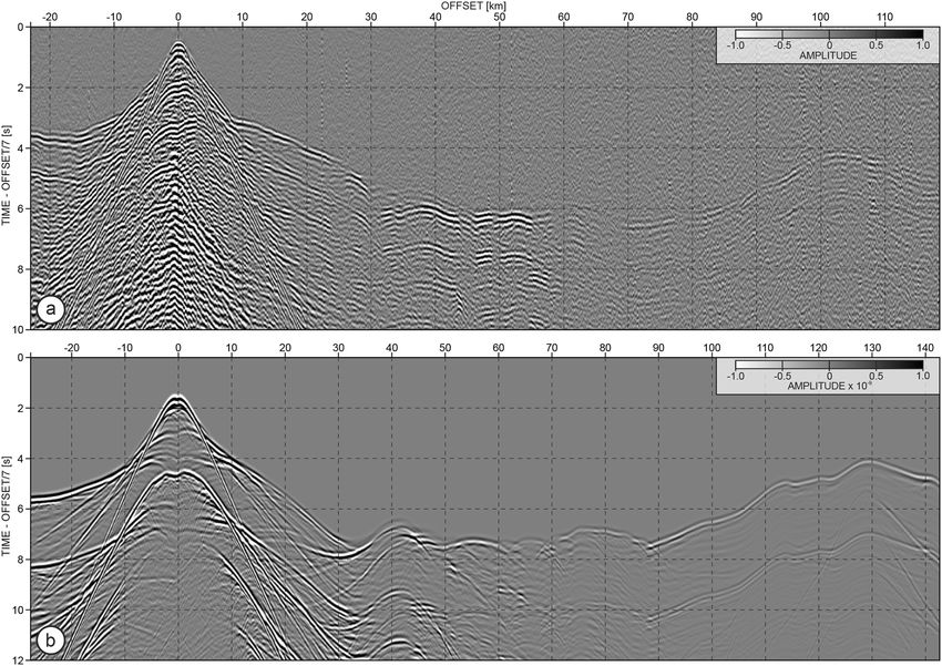
A. Górszczyk and S. Operto: GO_3D_OBS                                                                                                 1779

Figure 3. (a) Geometry of the major fault planes in the model (nodes at every 5 km are marked). (b) Projection of the initial structure from
Fig. 2a into 3D (sections at every 20 km are extracted). (c–f) Crossline sections extracted at 40, 70, 100, and 130 km – vertical red dashed
lines in Fig. 2a.

Therefore, the projection function applied to the second in-            plicitly coupled via the dependencies between the position
terface must be partially determined by the fact that one of            of the nodes which define them. Therefore, adding new fea-
the nodes (which belongs also to the first interface) was al-           tures to the model or modifying existing ones requires careful
ready projected. In such a way, the structural skeleton we              design of the corresponding projection functions, which will
create can be viewed as a system of interfaces that are im-             honour the previous dependencies between interfaces.

https://doi.org/10.5194/gmd-14-1773-2021                                                    Geosci. Model Dev., 14, 1773–1799, 2021
1780                                                                               A. Górszczyk and S. Operto: GO_3D_OBS

   We assumed that the model will be 100 km in width, there-        matrix containing the digitized accretionary block shown in
fore we generate 4001 2D inline sections spaced 25 m apart.         Fig. 2b, we reshape its geometry such that it fits to that of the
To highlight the lateral variability of the structure gener-        corresponding polygon (red shaded area in Fig. 2a) in each
ated during the projection, we show the skeleton of the in-         projected inline section. The deformed sediment layers in-
line sections in a perspective view extracted every 20 km           side the outer wedge have indexes consistent with those of
(Fig. 3b). First, we design the curved shape of the subduc-         the sediment layers coming into the trench since they repre-
tion front. With increasing crossline distance, the oceanic         sent the same geological formations. Filling all the polygons
crust and mantle shrink back. As a result, the continental          with the corresponding indexes leads to the matrix plotted in
part of the mantle and crust elongates seaward. Simultane-          Fig. 4a. We pick random colours to distinguish between the
ously, we compress and extend the respective polygons mak-          neighbouring units. The matrix contains 46 geological blocks
ing their relative size variable. One can track this variability    defined by the unique integer index. Such indexation allows
by following the geometry of the interfaces cutting through         us to easily refer to a particular structural unit of the model
the oceanic mantle and crust along successive inline sections       during the further steps – for example to modify the parame-
(blue dashed lines in Fig. 3b). The absolute depth of the           terization.
oceanic crust not only changes along the subduction trend              On top of the index matrix, we implement another matrix,
but also gently increasing with crossline distance. Simultane-      referred to as gradient matrix, which allows us to introduce
ously, there is an up-growing of the underplating sediments         spatial variations in the physical parameters in each large-
below the edge of the continental crust (black dashed lines         scale unit and around the main fault planes (Fig. 4b). Without
in Fig. 3b) – consistent with the thickening of the subduct-        this second matrix, the physical parameters in each geolog-
ing sediments as the crossline distance increases. The posi-        ical unit would have constant value (related to the integer
tion of the backstop also changes from one inline to another.       from matrix of indexes). The spatial variation in the param-
This partially results from the curved shape of the subduc-         eters within the same unit can be related to increasing depth
tion front and was inspired by the 3D interpretation of Tsuji       in the mantle, layering of the crust, low-velocity zones in the
et al. (2017). At the same time, the length of the inner wedge      subducting sediments, compaction in the prism or damage
(solid blue lines) increases. This is coupled with the differ-      zones around the faults, etc. We implement those variations
ences in scale and deformation of the thrusts sheets that are       using horizontal and/or vertical gradient functions (i.e. linear
building this unit, as well as with the shape of the forearc        interpolation functions). These functions can be easily modi-
basin covering it. Further seaward, the outer wedge (i.e. ac-       fied and hence provide the necessary flexibility to update the
cretionary prism – red shaded polygon) becomes shorter and          variations in the physical parameters in the structural units.
thicker as the crossline distance is increasing. The right flank    The gradients in Fig. 4b contain float values, which are nor-
of the model is marked by the uplift of the bathymetry re-          malized between 0 and 1 for each unit. The exceptions are
lated to the presence of the incoming volcanic ridge which          the three units in the oceanic mantle (which do not reach the
becomes smaller as the crossline distance increases.                bottom of the model), as well as shallow sedimentary layers
   In Fig. 3c–f, the crossline sections extracted at 40, 70, 100,   and water column (no gradient implementation).
and 130 km (vertical red dashed lines in Fig. 2a) highlight the        In practice, the index matrix and the gradient matrix are
structural heterogeneity in the crossline direction. This het-      combined to implement any physical parameter in each ge-
erogeneity is defined at different scales. Firstly, due to the      ological formation. To do so, we extract a given geological
overall curved shape of the subducting front. Secondly, due         unit (based on the index matrix) and assign to it a constant
to the different projection functions causing warping of the        parameter value pα . We also extract the corresponding part
polygons. The structural complexity will be further increased       of the gradient matrix and denote it by Gn (normalized gra-
through parameterization and the application of stochastic          dient matrix). The gradient function associated with Gn can
components.                                                         be manipulated (scaled, clipped, biased, etc.) leading to the
                                                                    matrix G which provides a desired spatial variation in a pa-
2.3     Parameterization                                            rameter in a geological unit. The overall formula to compute
                                                                    the physical parameters inside a given model unit is as fol-
2.3.1    Index and gradient matrix                                  lows:
                                                                    p(x, z) = pα + pβ g(x, z),                                   (2)
Once the inline section has been projected in the crossline di-
rection, the newly generated structural skeletons are further       where p(x, z) is the parameter entry at the position (x, z),
mapped into uniform 2D Cartesian grids of the dimension             while pβ scales the entry g(x, z) of G with appropriate phys-
1201 × 7001 (grid size 25 m × 25 m). During this step, we           ical units.
assign an arbitrary index to the grid points representing dif-         To better illustrate how the index and gradient matrix can
ferent geological units. That is, the grid points inside each of    be used to produce a physical model, we consider the fol-
the polygons are now described by a unique integer value.           lowing example. Let us imagine that we want to assign Vp
By re-sampling, in the horizontal and vertical directions, the      values inside the part of the oceanic crust delineated by the

Geosci. Model Dev., 14, 1773–1799, 2021                                              https://doi.org/10.5194/gmd-14-1773-2021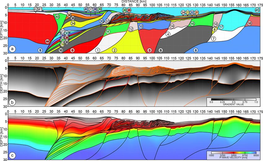
A. Górszczyk and S. Operto: GO_3D_OBS                                                                                              1781

Figure 4. (a) Index matrix with the 46 geological units marked by randomly picked colours. (b) Gradient matrix used for implementation of
spatial variations within those units. (c) 2D inline obtained after assigning Vp values to the matrices shown in (a, b).

thick red line in Fig. 4a and b. The integer index assigned to         related damage zones, and subducting channel, which re-
this unit is 11 (Fig. 4a). We set pα to 4800 m s−1 and pβ to           sult from small-scale geological processes (fluid migrations,
2300 m s−1 . Taking into account that the values of Gn for this        lithological variations, tectonic compaction, mass wasting,
unit span 0.0 to 1.0 (from the top to the bottom of the crust),        etc.; Agudelo et al., 2009; Park et al., 2010). Moreover, we
the final Vp values will be increasing linearly from 4800 to           implement lateral parameter discontinuities at the interfaces
7100 m s−1 . One may also desire to implement a gradient dis-          acting as faults. For example, the stairs in the Moho result-
continuity in the oceanic crust corresponding to the oceanic           ing from the interfaces cutting through the oceanic mantle
layer 2–layer 3 boundary. Setting the thickness ratio to 0.3           and crust imply that the gradients on both sides of those in-
and 0.7 in layer 2 and layer 3 respectively would split Gn in          terfaces are slightly different. In consequence, we create a
unit 11 into two sub-matrices given by                                 lateral jump in the parameter values on both sides of the
                                                                      fault, which will generate impedance contrast amenable to its
   G1 = Gn /0.3;             0.0 ≤ Gn < 0.3,                           imaging. In practice, this jump is more pronounced near the
                                                            (3)
   G2 = (Gn − 0.3)/0.7; 0.3 ≤ Gn < 1.0.                                top of the mantle (∼ 5 to ∼ 7 km below Moho) and vanishes
                                                                       with increasing depth to completely disappear at the bottom
As a result, we obtain two gradient matrices G1 and G2 with            of the model.
normalized values between 0.0 and 1.0. We can now set the                 Finally, the gradient matrix also describes two additional
pα to 4800 m s−1 and pβ to 1600 m s−1 for G1 . As a result,            types of perturbations. The first type is implemented around
we obtain rapid increase in Vp between 4800 to 6400 m s−1              the regions of thickened oceanic crust mimicking subduct-
inside layer 2. For G2 , we use pα equal to 6500 m s−1 and pβ          ing volcanic ridges (Park et al., 2004; Kodaira, 2000). They
equal to 600 m s−1 leading to Vp values inside layer 3 rang-           are marked by the gradient and velocity variations in Fig. 4b
ing between 6500 and 7100 m s−1 . The resulting boundary               and c (95–105 and 145–155 km). The second type of pertur-
between layer 2 and layer 3 is marked with dashed line in              bations is intended to introduce more heterogeneity around
Fig. 4c.                                                               the fault planes such as damage zones or fluid paths. Param-
   We also use the gradient matrix to implement variations             eter variations within such zones affect the kinematic and
in the parameters within the subducting sediments, fault-

https://doi.org/10.5194/gmd-14-1773-2021                                                  Geosci. Model Dev., 14, 1773–1799, 2021
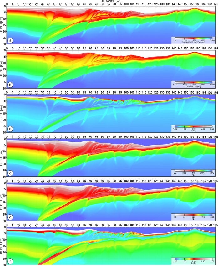
1782                                                                               A. Górszczyk and S. Operto: GO_3D_OBS

dynamic characteristic of the propagating wavefield. They              From the Vp model, we build Vs and ρ using the empirical
also have the potential to generate distinct arrivals – so-called   polynomial relations of Brocher (2005). These relations were
trapped waves (Li and Malin, 2008; Ben-Zion and Sammis,             inferred from compiled data on laboratory measurements,
2003). We implement such anomalies around the faults in the         logs, vertical seismic profiling, and tomographic studies.
oceanic crust and upper mantle, the major faults at the edge        They are relevant for Vp ranging from 1500 to 8500 m s−1
of continental crust, and within the large thrusts sheets be-       and hence represent the average behaviour of crustal rocks
tween inner and outer accretionary wedge. A few small per-          over the depth range covered by our model. The resulting Vs
turbations are also locally added between layers of the inner       and ρ models are presented in Fig. 6a and b. Shear-wave ve-
wedge to increase the complexity of this unit.                      locities in the shallow sediments are as small as ∼ 530 m s−1 .
                                                                    Although even lower velocities can be found in the first few
2.3.2   Physical parameters                                         metres below the seabed, these values already impose sig-
                                                                    nificant challenges for wavefield modelling. In the oceanic
From the index and gradient matrices described in the previ-        crust, Vs increases from 2900 to 4000 m s−1 , while it starts
ous section, we can now implement the seismic properties in         at 4500 m s−1 on top of the upper mantle and gently in-
the structural units. In practice, this requires some constraints   creases with depth. Density of the oceanic and continental
on the parameters, which might come from field experiments          crust varies from 2500 to 3000 kg m−3 and from 2500 to
and laboratory measurements. Regional seismic studies of-           2900 kg m−3 respectively, while in the upper mantle ρ starts
ten lack resolution to directly map the reconstructed prop-         around 3200 kg m−3 . Figure 6c shows the Vp /Vs ratio, which
erties into the fine-scale structures of our model. Moreover,       varies from 1.6 to 3.0. Initially, the Vs model obtained from
they often ignore second-order parameters such as density           empirical relations of Brocher (2005) was not producing a
(ρ), attenuation (Qp and Qs ), and anisotropy to focus on the       heterogeneous Vp /Vs ratio in the subduction channel – as it
P-wave velocity (Vp ) reconstruction, which plays the lead-         can occur when fluid overpressure, fluid diffusion, or hydro-
ing role in the active seismic imaging and can be estimated         geologically isolated zones generate variation in the seismic
from the seismic data more precisely than for example den-          properties in the subduction channel (Kodaira et al., 2002;
sity or attenuation. Therefore, we first develop a Vp model         Collot et al., 2008; Ribodetti et al., 2011). Therefore, we ad-
from recent FWI case studies in the Nankai Trough. Then,            ditionally rescale the velocities in this unit using the index
we use this Vp model as a reference to build the other pa-          and gradient matrices.
rameters – namely Vs , ρ, Qp , Qs – from empirical relations.          We also implement attenuation effects in our model
Reconstruction of Vp from wide-angle seismic data has long          through the Qp and Qs parameters. The choice of consistent
historical records (Christensen and Mooney, 1995; Mooney            approach to constrain plausible Qp and Qs models is quite
et al., 1998). Travel time tomography has produced a vast           challenging. This is firstly because the various types of at-
catalogue of smooth Vp models from different regions around         tenuation (intrinsic and scattering-related) can be controlled
the world. This information (even though Vp values can sig-         by countless factors – rock type and mineralogy, porosity,
nificantly vary depending on the studied area) is useful to         fluid content and saturation, temperature, etc. Secondly, val-
constrain the velocity trend in the main large-scale geolog-        ues of the Q factor can differ significantly between studies
ical units (such as mantle, continental, and oceanic crust).        depending on the methodology used, the scale of the attenu-
Moreover, recent OBS FWI case studies partially fill this           ation, or the frequency content of seismic data. Thirdly, ac-
resolution gap (Kamei et al., 2012; Górszczyk et al., 2017)         curate reconstruction of Q models from field experiments
and allow us to refine Vp in the short-scale units of our           is not as well documented because the footprint of atten-
model (Fig. 4c). We perform this refining of the Vp veloc-          uation in the wavefield remains small in particular in the
ities by trial and error, until the OBS gathers simulated un-       deep crust. Therefore, to build the Qp and Qs models, we
der acoustic approximation in the Vp model exhibit overall          combine few empirical relations between velocity (Vp , Vs ,
a similar anatomy to the OBS gathers collected during 2001          Vp /Vs ) and attenuation (Qp , Qs ), which we find consis-
Seize France Japan (SFJ) OBS survey in the eastern Nankai           tent for our synthetic model. To build the Qs model, we
Trough. In Fig. 5a and b, we present a qualitative compar-          use the following power law Qs = 0.0053 Vs1.25 (Wiggens
ison of the field and synthetic gathers for the OBS stations        et al., 1978). This empirical relation is in good agreement
located above the backstop of the Tokai segment and the             with the Qs estimation of Olsen et al. (2003) performed
backstop of the velocity model presented in Fig. 4c (30 km          in the Los Angeles Basin. The estimated Qs values range
of model distance). Despite the different offset ranges and         from ∼ 25 in the shallowest sediments to ∼220 in the deep
recording times (we extend it for the synthetic data to com-        mantle (see Fig. 6e). To avoid a constant ratio between
pensate for the deeper water than in the field data), the syn-      Qp and Qs (Qp = 1.5Qs in Olsen et al., 2003), we gener-
thetic gather exhibits the same types of arrivals appearing in      ated the Qp model (Fig. 6d) via another empirical relation
relatively similar order as in the case of the field data. This     Qp = 36.8(Vp )−49.6 – derived from well-log data by Zhang
similarity justifies a sufficient level of kinematic realism of     and Stewart (2008). This formula, even though derived from
the Vp values for the purpose of our geomodel.                      velocities up to ∼ 3000 m s−1 using a sonic-log frequency

Geosci. Model Dev., 14, 1773–1799, 2021                                             https://doi.org/10.5194/gmd-14-1773-2021
A. Górszczyk and S. Operto: GO_3D_OBS 1783
Figure 5. Comparison of the (a) field and (b) synthetic OBS gathers. The gather in (a) comes from the OBS 21 of the SFJ OBS 2001
experiment, while the gather in (b) comes from the waveform modelling for the OBS located at 30 km model distance of the 2D inline model
presented in Fig. 4c.
band, produces reasonable Qp variations between ∼ 35 and tended to introduce perturbations of a random character into
∼ 260 in our model and leads to a Qp /Qs ratio ranging from the model. We design two types of such random components:
∼ 1.1 to ∼ 1.5 (Fig. 6f), which is in good agreement with (i) small-scale parameter perturbations and (ii) spatial warp-
the values estimated in the Mariana subduction zone (Poz- ing of the final 3D cube.
gay et al., 2009). The small Q values in the shallow sediment
layers and/or subducting channel will significantly affect the 2.4.1 Small-scale perturbations
short to intermediate offset wavefield. On the other hand, the
higher Q values in the crust and mantle can still affect the In Figs. 4c and 6, the parameters vary smoothly within the
ultra-long-offset waves penetrating for a long time through units according to the applied gradient functions. Indeed,
these parts of the model. The Q values we define here are re- such smooth variations are a rather idealized vision of the
lated to the intrinsic attenuation during the wavefield propa- true earth. Therefore, to make it more realistic, we create an-
gation. Additionally, the attenuation of high-frequency wave- other matrix describing small-scale perturbations (Fig. 7a),
field component through the scattering effects is introduced which will have a second-order impact on the wavefield prop-
in our model by the means of small-scale stochastic pertur- agation. Using this matrix, we can scale the models after
bations as described in the following section. parameterization and obtain the updated model presented in
Fig. 7b (compare with the smooth velocity variations in the
2.4 Stochastic components Vp model shown in Fig. 4c). The inset in Fig. 7b shows the
symmetric histogram (with a distribution close to normal) of
In the final step of our model-building procedure, we con- the introduced velocity changes ranging between −300 to
sider various types of stochastic components, which are in- 300 m s−1 . The matrix in Fig. 7a is obtained by stacking 3D
https://doi.org/10.5194/gmd-14-1773-2021 Geosci. Model Dev., 14, 1773–1799, 20211784 A. Górszczyk and S. Operto: GO_3D_OBS Figure 6. (a) Vs , (b) ρ, (c) Vp /Vs , (d) Qp , (e) Qs , (f) Qp /Qs models derived from the Vp inline from Fig. 4c. disk-shaped structural elements (SEs) (Fig. 7c–f). The val- In Fig. 7c–f, we show four different 3D stacks (10 km × ues in the SEs (Fig. 7g) vary from 0 at the edge to 1 at the 10 km × 10 km sub-volumes are displayed), corresponding to centre and are further translated into parameter perturbations. four different scales of the SEs with a correlation length ratio We can control the position and size of these SEs, as well as equal to 0.25 × 1 × 1. The red/blue colours correspond to the their correlation lengths (z, x, y) – depending on a desired positive/negative amplitudes, which are randomly assigned characteristic of the final perturbations. to each of the SEs during stacking. These random variations Geosci. Model Dev., 14, 1773–1799, 2021 https://doi.org/10.5194/gmd-14-1773-2021
A. Górszczyk and S. Operto: GO_3D_OBS                                                                                                      1785

Figure 7. (a) Matrix of stochastic perturbations for a 2D inline section. (b) Vp model shown in Fig. 4c after the application of the stochastic
perturbations shown in (a). (c–f) 3D stack of structural elements of different scales – see the correlation lengths in brackets. Red/blue colours
indicate positive/negative magnitudes of the stacked structural elements. (g) Shape of the 3D structural element used to generate the stochastic
perturbations. (h, i) Wavenumber spectrum of the 2D Vp inline section with and without stochastic perturbations.

in positive/negative amplitudes guarantee that the final dis-              ry are the spatial shifts randomly picked from the intervals
tribution of the stochastic perturbations for each geological              (−z/4, z/4), (−x/4, x/4), and (−y/4, y/4). In other words,
unit in the matrix shown in Fig. 7a has a zero mean. The po-               the neighbouring SEs strongly overlap each other – as can be
sition of the SE within the stack is controlled by the Cartesian           seen in Fig. 7c.
coordinates. The distances between the centres of neighbour-                  Looking at the stochastic matrix in Fig. 7a, one can ob-
ing SE equal (z/2 + rz , x/2 + rx , y/2 + ry ), where rz , rx , and        serve that the scale, shape, and direction of the perturba-

https://doi.org/10.5194/gmd-14-1773-2021                                                       Geosci. Model Dev., 14, 1773–1799, 2021
1786                                                                              A. Górszczyk and S. Operto: GO_3D_OBS

tions vary from one geological unit to another. For example,       2.4.2   Structure warping
perturbations in the prism are finer than those in the crust
or mantle. Also, their shape in the oceanic crust and prism        Finally, we apply a second type of stochastic components to
are more anisotropic than the shape of those implemented in        the model after projection, parameterization, and application
the mantle. In practice, this is implemented by summation          of small-scale stochastic perturbations. The aim of this step
of 3D stacks containing different SEs. For example, we cre-        is to perform a small-scale pointwise warping of the input 3D
ate stochastic perturbations in the sedimentary layer and the      grid using a distribution of random shifts. By small-scale we
outer prism with only the SEs shown in Fig. 7e and f. Per-         mean that the structural changes introduced by warping are
turbations in the inner wedge and underplated units addition-      in general much smaller than those incorporated during the
ally incorporate SEs shown in Fig. 7d. Finally, the oceanic        projection step. Their impact on the shape of the wavefield
crust contains SEs at all scales (Fig. 7c–f). This also applies    will therefore be weaker than the one induced by the geolog-
to the mantle and continental crust; however, for these units      ical structure itself but more pronounced than that resulting
we use an SE with different correlation length ratios equal to     from the small-scale perturbations described in the previous
0.5 × 1 × 1. Due to the strong overlapping of the SEs and the      section. The idea was inspired by dynamic image warping
superposition of SEs of different scales, the range of the mag-    (DIW) (Hale, 2013). DIW is a technique which allows for
nitude inside the final 3D stacks significantly exceeds ±1.        the estimation of local shifts between two images (2D matri-
Therefore, after staking procedure, we re-normalize the 3D         ces), assuming that one of the images is a warped version of
stochastic perturbation matrices between −1 and 1.                 the other image. This problem is cast as an inverse problem
   In Fig. 7a, we also show that the stochastic perturbations      where the unknowns are the shifts that will allow for match-
in some of the units are oriented according to the dipping         ing between the two images.
or bending of the structure. Since we know the polynomials            In our case, we use DIW in a forward sense. This means
defining each of the interfaces in the model (and therefore        we build a matrix of smoothly varying random spatial shifts
their position), we shift vertically the columns of the matrix     of a desired scale and magnitude. Then, we warp each of the
containing stochastic perturbations of a given geological unit     inline section from the 3D model grid using those shifts. Fig-
such that they follow the shape of the structure. For example,     ure 8a and b show two 300 km × 300 km matrices that rep-
the perturbations that fill the oceanic crust follow the smooth    resent distribution of shifts for two different spatial scales.
trend generated from the polynomial approximation of the           While the scale of the shifts in Fig. 8a is local (starting from
interfaces creating the top of the oceanic crust. Note, that be-   ∼ 10 km), the spatial extension of the shifts in Fig. 8b is re-
cause we stack truly 3D SE, within the 3D cube of the same         gional. The blue and red colours indicate the negative and
size as the 3D model, our stochastic perturbations continu-        positive shifts respectively – scaled between ±2 km. To ob-
ously follow the geological structures not only in the inline      tain those matrices, we first generate the matrix of the same
direction but also in the crossline direction.                     size with the random values from the (−1, 1) interval. In the
   To analyse what the designed stochastic perturbations           second step we interpolate between the uniformly subsam-
mean in terms of the spatial resolution of the model, we com-      pled (in both directions) elements of this random matrix us-
pute the 2D wavenumber spectrum (displayed in logarithmic          ing spline functions. The spatial scale of the final shifts is
amplitude scale in Fig. 7h, i) of the Vp model with and with-      controlled by the subsampling of the matrix with random val-
out stochastic components. As shown in Fig. 7h, the spectral       ues – that is, the dense or sparse subsampling leads to small-
amplitudes of the model without stochastic perturbations are       or large-scale of perturbations. After interpolation, we scale
focused around the low-wavenumber part of the spectrum,            the values in both matrices to obtain the desired magnitude of
which represents structures the size of which is of the order      the shifts (in this case ±2 km). We take the average of the two
of ∼ 500 m and larger. In contrast, the high-wavenumber am-        distributions to obtain the final distribution shown in Fig. 8c.
plitudes are clearly magnified in the spectrum of the model        Our procedure of warping is implemented as follow.
with stochastic components (Fig. 7i). The overall spatial dis-        First, for each of the 4001 inline sections, we extract from
tribution of the energy added to the background medium with        the distribution shown in Fig. 8c a 2D sub-matrix with the
respect to the spectrum shown in Fig. 7h is broad, which           size of the inline section. Figure 8d shows such a matrix
highlights the randomness of the perturbations. The designed       corresponding to the first inline section – marked by to the
approach led to perturbations of a smaller size in fact being      black-dashed rectangle in the upper-right corner of Fig. 8c.
of the order of the grid size (25 m). On the other hand, one       The further rectangles in Fig. 8c illustrate how we move from
can also observe in Fig. 7i a few dipping bands of increased       one sub-matrix to another one for five inline sections spaced
amplitudes. They correspond to the anisotropic shape of the        20 km apart (inline number 1, 1001, 2001, 3001, and 4001).
SEs following the geological structures – and therefore indi-         Once we have the sub-matrix of shifts and the initial in-
cate that our stochastic perturbations are partially predefined    line section mi (x, z), the warped inline section mw (x, z) is
and not purely random.                                             obtained by the identity mw (x, z) = mi (x, z + s), where s is
                                                                   the entry of the sub-matrix of shifts at the (x, z) position. In
                                                                   Fig. 8d, the warped structure (dashed black lines) is shifted

Geosci. Model Dev., 14, 1773–1799, 2021                                            https://doi.org/10.5194/gmd-14-1773-2021
You can also read