Intercomparison of MAX-DOAS vertical profile retrieval algorithms: studies on field data from the CINDI-2 campaign - AMT
←
→
Page content transcription
If your browser does not render page correctly, please read the page content below
Atmos. Meas. Tech., 14, 1–35, 2021
https://doi.org/10.5194/amt-14-1-2021
© Author(s) 2021. This work is distributed under
the Creative Commons Attribution 4.0 License.

Intercomparison of MAX-DOAS vertical profile retrieval
algorithms: studies on field data from the CINDI-2 campaign
Jan-Lukas Tirpitz1 , Udo Frieß1 , François Hendrick2 , Carlos Alberti3,a , Marc Allaart4 , Arnoud Apituley4 , Alkis Bais5 ,
Steffen Beirle6 , Stijn Berkhout7 , Kristof Bognar8 , Tim Bösch9 , Ilya Bruchkouski10 , Alexander Cede11,12 ,
Ka Lok Chan3,b , Mirjam den Hoed4 , Sebastian Donner6 , Theano Drosoglou5 , Caroline Fayt2 , Martina M. Friedrich2 ,
Arnoud Frumau13 , Lou Gast7 , Clio Gielen2,c , Laura Gomez-Martín14 , Nan Hao15 , Arjan Hensen13 , Bas Henzing13 ,
Christian Hermans2 , Junli Jin16 , Karin Kreher18 , Jonas Kuhn1,6 , Johannes Lampel1,19 , Ang Li20 , Cheng Liu21 ,
Haoran Liu21 , Jianzhong Ma17 , Alexis Merlaud2 , Enno Peters9,d , Gaia Pinardi2 , Ankie Piters4 , Ulrich Platt1,6 ,
Olga Puentedura14 , Andreas Richter9 , Stefan Schmitt1 , Elena Spinei12,e , Deborah Stein Zweers4 , Kimberly Strong8 ,
Daan Swart7 , Frederik Tack2 , Martin Tiefengraber11,22 , René van der Hoff7 , Michel van Roozendael2 , Tim Vlemmix4 ,
Jan Vonk7 , Thomas Wagner6 , Yang Wang6 , Zhuoru Wang15 , Mark Wenig3 , Matthias Wiegner3 , Folkard Wittrock9 ,
Pinhua Xie20 , Chengzhi Xing21 , Jin Xu20 , Margarita Yela14 , Chengxin Zhang21 , and Xiaoyi Zhao8,f
1 Institute of Environmental Physics, University of Heidelberg, Heidelberg, Germany
2 Royal  Belgian Institute for Space Aeronomy, Brussels, Belgium
3 Meteorological Institute, Ludwig-Maximilians-Universität München, Munich, Germany
4 Royal Netherlands Meteorological Institute (KNMI), De Bilt, the Netherlands
5 Laboratory of Atmospheric Physics, Aristotle University of Thessaloniki, Thessaloniki, Greece
6 Max Planck Institute for Chemistry, Mainz, Germany
7 National Institute for Public Health and the Environment (RIVM), Bilthoven, the Netherlands
8 Department of Physics, University of Toronto, Toronto, Canada
9 Institute for Environmental Physics, University of Bremen, Bremen, Germany
10 National Ozone Monitoring Research and Education Center (NOMREC), Belarusian State University, Minsk, Belarus
11 LuftBlick Earth Observation Technologies, Mutters, Austria
12 NASA-Goddard Space Flight Center, Greenbelt, MD, USA
13 Netherlands Organisation for Applied Scientific Research (TNO), Utrecht, the Netherlands
14 National Institute of Aerospatial Technology (INTA), Madrid, Spain
15 Remote Sensing Technology Institute, German Aerospace Center (DLR), Oberpfaffenhofen, Germany
16 Meteorological Observation Centre, China Meteorological Administration, Beijing, China
17 Chinese Academy of Meteorology Science, China Meteorological Administration, Beijing, China
18 BK Scientific GmbH, Mainz, Germany
19 Airyx GmbH, Justus-von-Liebig-Straße 14, Eppelheim, Germany
20 Anhui Institute of Optics and Fine Mechanics, Chinese Academy of Sciences, Hefei, China
21 School of Earth and Space Sciences, University of Science and Technology of China, Hefei, China
22 Department of Atmospheric and Cryospheric Sciences, University of Innsbruck, Innsbruck, Austria
a now at: Institute of Meteorology and Climate Research (IMK-ASF),

Karlsruhe Institute of Technology (KIT), Karlsruhe, Germany
b now at: Remote Sensing Technology Institute (IMF), German Aerospace Center (DLR), Oberpfaffenhofen, Germany
c now at: Institute for Astronomy, KU Leuven, Leuven, Belgium
d now at: Institute for Protection of Maritime Infrastructures, Bremerhaven, Germany
e now at: Virginia Polytechnic Institute and State University, Blacksburg, VA, USA
f now at: Air Quality Research Division, Environment and Climate Change Canada, Vancouver, Canada

Correspondence: Jan-Lukas Tirpitz (jan-lukas.tirpitz@iup.uni-heidelberg.de)

Published by Copernicus Publications on behalf of the European Geosciences Union.
2                                                                          J.-L. Tirpitz et al.: CINDI-2 profiling comparison

Received: 27 November 2019 – Discussion started: 2 January 2020
Revised: 23 October 2020 – Accepted: 5 November 2020 – Published: 4 January 2021

Abstract. The second Cabauw Intercomparison of Nitro-              trace gas VCDs from direct-sun DOAS observations and
gen Dioxide measuring Instruments (CINDI-2) took place in          (0.8–9) × 1010 molec. cm−3 against surface concentrations
Cabauw (the Netherlands) in September 2016 with the aim            from the long-path DOAS instrument. This increase in
of assessing the consistency of multi-axis differential opti-      RMSDs is most likely caused by uncertainties in the sup-
cal absorption spectroscopy (MAX-DOAS) measurements of             porting data, spatiotemporal mismatch among the observa-
tropospheric species (NO2 , HCHO, O3 , HONO, CHOCHO                tions and simplified assumptions particularly on aerosol op-
and O4 ). This was achieved through the coordinated opera-         tical properties made for the MAX-DOAS retrieval.
tion of 36 spectrometers operated by 24 groups from all over          As a side investigation, the comparison was repeated with
the world, together with a wide range of supporting reference      the participants retrieving profiles from their own differ-
observations (in situ analysers, balloon sondes, lidars, long-     ential slant column densities (dSCDs) acquired during the
path DOAS, direct-sun DOAS, Sun photometer and meteo-              campaign. In this case, the consistency among the partici-
rological instruments).                                            pants degrades by about 30 % for AOTs, by 180 % (40 %) for
   In the presented study, the retrieved CINDI-2 MAX-              HCHO (NO2 ) VCDs and by 90 % (20 %) for HCHO (NO2 )
DOAS trace gas (NO2 , HCHO) and aerosol vertical pro-              surface concentrations.
files of 15 participating groups using different inversion algo-      In former publications and also during this comparison
rithms are compared and validated against the colocated sup-       study, it was found that MAX-DOAS vertically integrated
porting observations, with the focus on aerosol optical thick-     aerosol extinction coefficient profiles systematically under-
nesses (AOTs), trace gas vertical column densities (VCDs)          estimate the AOT observed by the Sun photometer. For the
and trace gas surface concentrations. The algorithms are           first time, it is quantitatively shown that for optimal estima-
based on three different techniques: six use the optimal es-       tion algorithms this can be largely explained and compen-
timation method, two use a parameterized approach and one          sated by considering biases arising from the reduced sensi-
algorithm relies on simplified radiative transport assumptions     tivity of MAX-DOAS observations to higher altitudes and
and analytical calculations. To assess the agreement among         associated a priori assumptions.
the inversion algorithms independent of inconsistencies in
the trace gas slant column density acquisition, participants
applied their inversion to a common set of slant columns.
Further, important settings like the retrieval grid, profiles of   1   Introduction
O3 , temperature and pressure as well as aerosol optical prop-
erties and a priori assumptions (for optimal estimation algo-      The planetary boundary layer (PBL) is the lowest part of
rithms) have been prescribed to reduce possible sources of         the atmosphere, whose behaviour is directly influenced by
discrepancies.                                                     its contact with the Earth’s surface. Its chemical composi-
   The profiling results were found to be in good qualitative      tion and aerosol load are driven by the exchange with the
agreement: most participants obtained the same features in         surface, transport processes and homogeneous and hetero-
the retrieved vertical trace gas and aerosol distributions; how-   geneous chemical reactions. Monitoring of both trace gases
ever, these are sometimes at different altitudes and of differ-    and aerosols, preferably simultaneous, is crucial for the un-
ent magnitudes. Under clear-sky conditions, the root-mean-         derstanding of the spatiotemporal evolution of the PBL com-
square differences (RMSDs) among the results of individ-           position and the chemical and physical processes.
ual participants are in the range of 0.01–0.1 for AOTs, (1.5–         Multi-axis differential optical absorption spectroscopy
15) ×1014 molec. cm−2 for trace gas (NO2 , HCHO) VCDs              (MAX-DOAS) (e.g. Hönninger and Platt, 2002; Hönninger
and (0.3–8) × 1010 molec. cm−3 for trace gas surface con-          et al., 2004; Wagner et al., 2004; Heckel et al., 2005; Frieß
centrations. These values compare to approximate average           et al., 2006; Platt and Stutz, 2008; Irie et al., 2008; Clémer
optical thicknesses of 0.3, trace gas vertical columns of          et al., 2010; Wagner et al., 2011; Vlemmix et al., 2015b)
90 × 1014 molec. cm−2 and trace gas surface concentrations         is a widely used ground-based measurement technique for
of 11×1010 molec. cm−3 observed over the campaign period.          the detection of aerosols and trace gases particularly in the
The discrepancies originate from differences in the applied        lower troposphere: ultraviolet (UV) and visible (Vis) absorp-
techniques, the exact implementation of the algorithms and         tion spectra of skylight are analysed to obtain information
the user-defined settings that were not prescribed.                on different atmospheric absorbers and scatterers, integrated
   For the comparison against supporting observations, the         over the light path (in fact, a superposition of a multitude of
RMSDs increase to a range of 0.02–0.2 against AOTs from            light paths). The amount of atmospheric trace gases along
the Sun photometer, (11–55) × 1014 molec. cm−2 against             the light path is inferred by identifying and analysing their

Atmos. Meas. Tech., 14, 1–35, 2021                                                      https://doi.org/10.5194/amt-14-1-2021
J.-L. Tirpitz et al.: CINDI-2 profiling comparison                                                                              3

characteristic narrow spectral absorption features, applying      gaseS (BOREAS) algorithm were already compared against
DOAS (Platt and Stutz, 2008). Gases that have been analysed       supporting observations but regarding a few days only. Fi-
in the UV and Vis spectral ranges are nitrogen dioxide (NO2 ),    nally, it shall be mentioned that already in the course of the
formaldehyde (HCHO), nitrous acid (HONO), water vapour            precedent CINDI-1 campaign in 2009, there were compar-
(H2 O), sulfur dioxide (SO2 ), ozone (O3 ), glyoxal (CHO-         isons of MAX-DOAS aerosol extinction coefficient profiles,
CHO) and halogen oxides (e.g. BrO, OClO). The oxygen-             e.g. by Frieß et al. (2016) and Zieger et al. (2011); however,
collision-induced absorption (in the following treated as if      these are also over shorter periods and a smaller group of
it is an additional trace gas species, O4 ) can be used to in-    participants.
fer information on aerosols: since the concentration of O4 is        The paper is organized as follows: Sect. 2 introduces the
proportional to the square of the O2 concentration, its verti-    campaign setup, the MAX-DOAS dataset with the partici-
cal distribution is well known. The O4 absorption signal can      pating groups and algorithms (Sect. 2.1), the available sup-
therefore be utilized as a proxy for the light path with the      porting observations for validation (Sect. 2.2) and the general
latter being strongly dependent on the atmosphere’s aerosol       comparison strategy (Sect. 2.3). The comparison results are
content. An appropriate set of spectra recorded under a nar-      shown in Sect. 3. A compact summarizing plot and the con-
row field of view (FOV, full aperture angle around 10 mrad)       clusions appear in Sect. 4.
and different viewing elevations (“multi-axis”) provide in-
formation on the trace gas and aerosol vertical distributions.
Profiles can be retrieved from this information by applying       2     Instrumentation and methodology
numerical inversion algorithms, typically incorporating ra-
                                                                  Figure 1 shows an overview of the CINDI-2 campaign setup,
diative transfer models. These profile retrieval algorithms are
                                                                  including the supporting observations relevant for this study.
the subject of this comparison study.
                                                                  Instrument locations, pointing (remote sensing instruments)
   Today, there are numerous retrieval algorithms in regular
                                                                  and flight paths (radiosondes) are indicated on the map. De-
use within the MAX-DOAS community which rely on differ-
                                                                  tails on the instruments and their data products can be found
ent mathematical inversion approaches. This study involves
                                                                  in the following subsections. For further information, refer to
nine of these algorithms (listed in Table 2), of which six use
                                                                  Kreher et al. (2019) and Apituley et al. (2020).
the optimal estimation method (OEM), two use a parameter-
ized approach (PAR) and one relies on simplified radiative        2.1     MAX-DOAS dataset
transport assumptions and analytical calculations (ANA).
The main objective of this study is to assess their consis-       2.1.1    Underlying dSCD dataset
tency and to review strengths and weaknesses of the individ-
ual algorithms and techniques. Note that this study is strongly   Deriving vertical gas concentration and aerosol extinction
linked to the report by Frieß et al. (2019), who performed        profiles from scattered skylight spectra can be regarded as
similar investigations on nearly the same set of profiling al-    a two-step process: the first step is the DOAS spectral analy-
gorithms with synthetic data, whereas the underlying data         sis, where the magnitude of characteristic absorption patterns
here were recorded during the second Cabauw Intercompar-          of different gas species in the recorded spectra is quantified
ison for Nitrogen Dioxide measuring Instruments (CINDI-           to derive the so-called “differential slant column densities”
2; Apituley et al., 2020). The CINDI-2 campaign took place        (dSCDs; definition in the following paragraph). These pro-
from 25 August to 7 October 2016 on the Cabauw Experi-            vide information on integrated gas concentrations along the
mental Site for Atmospheric Research (CESAR; 51.9676◦ N,          lines of sight. The second step is the actual profile retrieval,
4.9295◦ E) in the Netherlands, which is operated by the           where inversion algorithms incorporating atmospheric radia-
Royal Netherlands Meteorological Institute (KNMI). In total,      tive transfer models (RTMs) are applied to retrieve concen-
36 spectrometers of 24 participating groups from all over the     tration profiles from the dSCDs derived in the first step.
world were synchronously measuring together with a wide              The very initial data in the MAX-DOAS processing chain
range of supporting observations (in situ analysers, balloon      are intensities of scattered skylight Iλ (α) at different wave-
sondes, lidars, long-path DOAS, direct-sun DOAS, Sun pho-         lengths λ (ultraviolet and visible spectral ranges, typical res-
tometer and meteorological instruments) for validation. This      olutions of 0.5 to 1.5 nm) recorded under different viewing
study compares MAX-DOAS profiles of NO2 and HCHO                  elevation angles α (ideally the telescope’s FOV is negligible
concentrations as well as the aerosol extinction coefficient      compared to the elevation angle resolution). Along the light
(derived from O4 observations) from 15 of the 24 groups. The      path l from the top of the atmosphere (TOA) to the instru-
results are compared with each other and validated against        ment on the ground, each atmospheric gas species i imprints
CINDI-2 supporting observations. For HONO and O3 profil-          its unique spectral absorption pattern (given by the absorp-
ing results, please refer to Wang et al. (2020) and Wang et al.   tion cross section σi,λ ) onto the TOA spectrum Iλ,TOA with
(2018), respectively. In a recent publication by Bösch et al.     the optical thickness
(2018), CINDI-2 MAX-DOAS profiles retrieved with the
Bremen Optimal estimation REtrieval for Aerosols and trace

https://doi.org/10.5194/amt-14-1-2021                                                     Atmos. Meas. Tech., 14, 1–35, 2021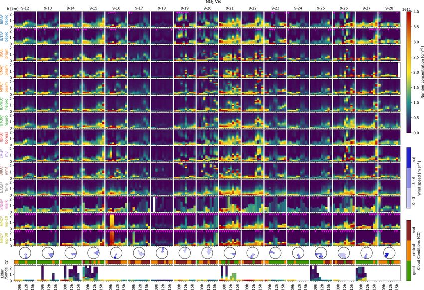
4                                                                                J.-L. Tirpitz et al.: CINDI-2 profiling comparison

Figure 1. Left: image of the CESAR site with position and approximate viewing directions of the MAX-DOAS instruments and supporting
observations of relevance for this study. Right: map with instrument locations, viewing geometries and sonde flight paths indicated (credit:
Esri 2018).

                                                                        dSCD results was conducted by Kreher et al. (2019). In the
                                                                      course of their study, Kreher et al. (2019) identified the most
                   Iλ,TOA            X
τλ (α) = log                     =    σi,λ Si (α) + C.         (1)      reliable instruments to derive a “best” median dSCD dataset.
                    Iλ (α)            i                                 This dataset – in the following referred to as the “median
                                                                        dSCDs” – was distributed among the participants. All par-
Si (α) is the slant column density (SCD), which is the trace            ticipants used the median dSCDs as the input data for their
gas concentration integrated along l. C represents terms ac-            retrieval algorithms and retrieved the profiles that are com-
counting for other instrumental and physical effects than               pared in this study. The “median dSCD” approach was cho-
trace gas absorption (for instance, scattering on molecules             sen for the following reasons: (i) it enables us to compare
and aerosols) that will not be further discussed in this con-           the profiling algorithms independently from differences in
text. Si (α) is inferred by spectrally fitting literature values        the input dSCDs, which is necessary to assess the individual
of σi,λ to the observed τλ (α). Since normally Iλ,TOA is not            algorithm performance; (ii) it makes this study directly com-
available for the respective instrument, optical thicknesses            parable to the report by Frieß et al. (2019). Among others,
are instead assessed with respect to the spectrum recorded              this allows us to assess to what extent MAX-DOAS profil-
in zenith viewing direction to obtain                                   ing studies on synthetic data (with lower effort) can be used

                  Iλ (α = 90◦ )
                                                                       to substitute studies on real data. (iii) Two decoupled studies
1τλ (α) = log                     .                          (2)        are obtained (Kreher et al., 2019 and this study), each con-
                      Iλ (α)                                            fined to a single step in the MAX-DOAS processing chain
Then the spectral fit yields the so-called differential slant col-      (the DOAS spectral analysis to obtain dSCDs and the actual
umn densities (dSCDs):                                                  profile inversion). A disadvantage of the median dSCD ap-
                                                                        proach is that the reliability of a typical MAX-DOAS ob-
1S(α) = S(α) − S(α = 90◦ ),                                    (3)      servation undergoing the whole spectra acquisition and pro-
                                                                        cessing chain cannot be assessed. Therefore, a comparison of
which are the typical output of the DOAS spectral analysis              profiles retrieved with the participant’s own dSCDs was also
when applied to MAX-DOAS data. For further details on the               conducted but is not a substantial part of this study. How-
DOAS method, refer to Platt and Stutz (2008).                           ever, these results and a corresponding short discussion can
   During the CINDI-2 campaign, each participant measured               be found in Supplement Sect. S10 and Sect. 3.7, respectively.
spectra with their own instrument and derived dSCDs ap-                 The median dSCDs cover the campaign core period from 12
plying their preferred DOAS spectral analysis software. The             to 28 September 2016, considering only data from the first
pointings (azimuthal and elevation) of all MAX-DOAS in-                 10 min of each hour between 07:00 and 16:00 UT, where the
struments were aligned to a common direction (Donner et al.,            CINDI-2 MAX-DOAS measurement protocol scheduled an
2019) and all participants had to comply with a strict mea-             elevation scan in the nominal 287◦ azimuth viewing direction
surement protocol, assuring synchronous pointing and spec-              with respect to the north. Hence, the total number of pro-
tra acquisition under highly comparable conditions (Apitu-              cessed elevation scans was 170. An elevation scan consisted
ley et al., 2020). A detailed comparison and validation of the

Atmos. Meas. Tech., 14, 1–35, 2021                                                             https://doi.org/10.5194/amt-14-1-2021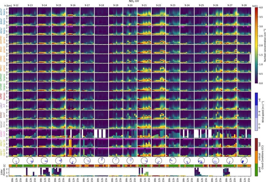
J.-L. Tirpitz et al.: CINDI-2 profiling comparison                                                                                5

of 10 successively recorded spectra at viewing elevation an-        achieved compared to other algorithms (factor of ≈ 103 in
gles α of 1, 2, 3, 4, 5, 6, 8, 15, 30 and 90◦ , at an acquisition   processing time; see Frieß et al., 2019).
time of 1 min each. dSCDs were provided for three chemical             For further descriptions of the methods and the individual
species, namely O4 , NO2 and HCHO. O4 and NO2 were each             algorithms, please refer to Frieß et al. (2019). Besides the
provided for two different spectral fitting ranges, in the UV       algorithms described therein, our study includes results from
and Vis spectral regions, resulting in five data products (see      the M 3 algorithm by LMU (see Table 2 for definition). Its
Table 1). From the median dSCDs, the participants retrieved         description can be found in Supplement Sect. S1. For details,
profiles for the species listed in Table 1. Not all participants    refer to the references given in Table 2.
retrieved all species and therefore do not necessarily appear          Note that two versions of aerosol results from the MAPA
in all plots.                                                       algorithm (see Table 2 for definition) with different O4 scal-
                                                                    ing factors (SFs) are discussed within this paper, referred to
                                                                    as mp-0.8 (retrieved with SF = 0.8) and mp-1.0 (SF = 1.0),
2.1.2   Participating groups and algorithms
                                                                    respectively. The scaling factor is applied to the measured
                                                                    O4 dSCDs prior to the retrieval and was initially motivated
Table 2 lists the compared algorithms including the under-          by previous MAX-DOAS studies which reported a signifi-
lying method (OEM, PAR or ANA) and the participating                cant yet debated mismatch between measured and simulated
groups with corresponding labels and plotting symbols as            dSCDs (e.g. Wagner et al., 2009; Clémer et al., 2010; Or-
they are used throughout the comparison. OEM and PAR al-            tega et al., 2016; Wagner et al., 2019, and references therein).
gorithms rely on the same idea: a layered horizontally ho-          Also for MAPA during CINDI-2, a scaling factor of 0.8 was
mogeneous atmosphere is set up in a RTM with distinct pa-           found to improve the dSCD agreement, enhance the num-
rameters (aerosol extinction coefficient, trace gas amounts,        ber of valid profiles and significantly improve the agreement
temperature, pressure, water vapour and aerosol properties)         with the Sun photometer aerosol optical thickness (Beirle
attributed to each layer. This model atmosphere is then used        et al., 2019). However, in the course of this study, it was
to simulate MAX-DOAS dSCDs under consideration of the               found that for OEM algorithms the disagreement between
viewing geometries. To retrieve a profile from the measured         Sun photometer and MAX-DOAS can largely be explained
dSCDs, the model parameters are optimized to minimize               by smoothing effects (see Sect. 3.4) and that (at least aver-
the difference between the simulated and measured dSCDs             aged over campaign) there are no clear indications that a SF
based on a predefined cost function.                                is necessary (see Supplement Sect. S2).
   Regarding profiles, typically only 2 to 4 degrees of free-
dom for signal (DOFS or p) can be retrieved from MAX-               2.1.3   Retrieval settings
DOAS observations, such that general profile retrieval prob-
lems with more than p independent retrieved parameters              To reduce possible sources of discrepancies, all profiles
are ill-posed and prior information has to be assimilated to        shown in this study were retrieved according to predefined
achieve convergence. For OEM algorithms, this is provided           settings similar to those of the intercomparison study by
in the form of an a priori profile and associated a priori co-      Frieß et al. (2019): pressure, temperature, total air density
variance (Rodgers, 2000), defining the most likely profile          and O3 vertical profiles between 0 and 90 km altitude were
and constraining the space of possible solutions according to       averaged from O3 sonde measurements performed in De Bilt
prior experience. They constitute a portion of the OEM cost         by KNMI during September months of the years 2013–2015.
function such that with decreasing information contained in         A fixed altitude grid was used for the inversion, consisting
the measurements, layer concentrations are drawn towards            of 20 layers between 0 and 4 km altitude, each with a height
their a priori values. PAR algorithms implement prior as-           of 1h = 200 m. The results of the parameterized approaches
sumptions by only allowing predefined profile shapes which          and OEM algorithms where the exact grid could not read-
can be described by a few parameters.                               ily be applied during inversion were interpolated and aver-
   For OEM algorithms, the radiative transport simulations          aged accordingly afterwards. Note that, for radiative transfer
are performed online in the course of the retrieval, whereas        simulations, the atmosphere was represented by finer (25 to
the PAR algorithms in this study rely on look-up tables,            100 m) layers close to the surface, increasing with altitude)
which are precalculated for the parameter ranges of interest.       and farther extending (up to 40 to 90 km altitude) grids, in-
Therefore, PAR algorithms are typically faster than OEM al-         herently defined by the individual retrieval algorithms. Sur-
gorithms but also require more memory. The ANA approach             face and instruments’ altitudes were fixed to 0 m, which is
by NASA was developed as a quick-look algorithm and as-             close to the real conditions: the CESAR site and most of
sumes a simplified radiative transport, based on trigonomet-        the surrounding area lie at 0.7 m b.s.l., whereas the instru-
ric considerations. Since the model equations can be solved         ments were installed at 0 to 6 m above sea level. The model
analytically for the parameters of interest, neither radiative      wavelengths were fixed according to Table 3. In the case of
transport simulation nor the calculation of look-up tables is       the HCHO retrieval, the aerosol profiles retrieved at 360 nm
necessary, and an outstanding computational performance is          were extrapolated to 343 nm using the mean Ångström expo-

https://doi.org/10.5194/amt-14-1-2021                                                       Atmos. Meas. Tech., 14, 1–35, 2021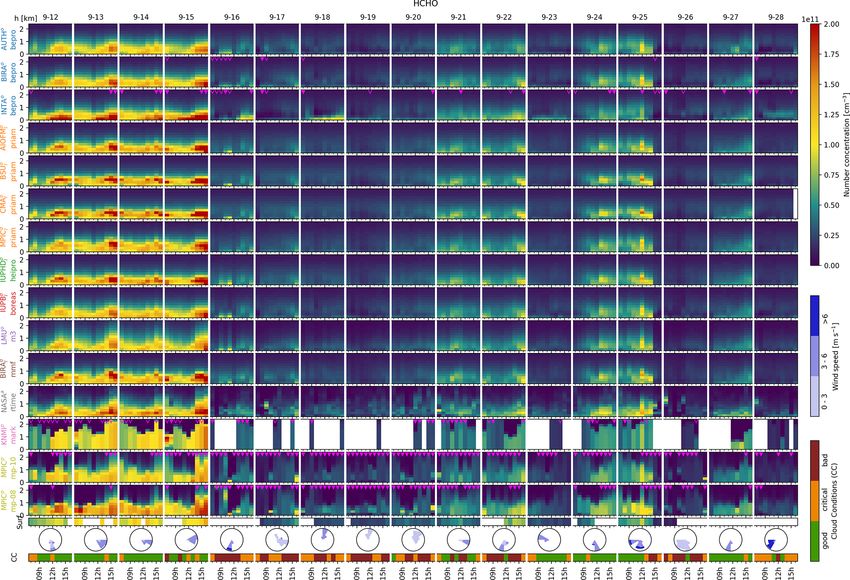
6                                                                                               J.-L. Tirpitz et al.: CINDI-2 profiling comparison

Table 1. List of the retrieved species and fitting ranges. For further details on the spectral analysis, please refer to Kreher et al. (2019).

                          Species            Retrieved quantity                                 Retrieved              Spectral fitting
                                                                                                from dSCDs of           window [nm]
                          Aerosol UV         Extinction coefficient [km−1 ]                     O4 UV                        338–370
                          Aerosol Vis        Extinction coefficient [km−1 ]                     O4 Vis                       425–490
                          NO2 UV             Number concentration [molec. cm−3 ]                NO2 UV                       338–370
                          NO2 Vis            Number concentration [molec. cm−3 ]                NO2 Vis                      425–490
                          HCHO               Number concentration [molec. cm−3 ]                HCHO                        336.5–359

Table 2. Groups who retrieved and provided profiling results for this study.

                        o OEM: optimal estimation. a ANA: analytical approach without radiative transfer model. p PAR: parameterized
                        approach. x IUPHD and UTOR used different versions of HEIPRO (1.2 and 1.5/1.4, respectively). y Two versions of
                        MAPA (labelled mp-10 and mp08) with different O4 scaling factors (0.8 and 1.0) are included in the comparison.
                        l Aerosol extinction is retrieved in logarithmic space. This removes negative values and allows larger values.

nent for the 440–675 nm wavelength range derived from Sun                            ing profiles with a scale height of 1 km and aerosol optical
photometer measurements (see Sect. 2.2.1) on 14 Septem-                              thicknesses (AOTs) and vertical column densities (VCDs) as
ber 2016 in Cabauw. For the aerosol parameters, the single                           given in Table 3. For the AOTs, the mean value at 477 nm for
scattering albedo was fixed to 0.92 and the asymmetry fac-                           the first days of September 2016 derived from AERONET
tor to 0.68 for both 360 and 477 nm. These are mean values                           measurements are used. Trace gas VCDs are mean values
for 14 September 2016 derived from Aerosol Robotic Net-                              derived from Ozone Monitoring Instrument (OMI) observa-
work (AERONET) measurements at 440 nm in Cabauw. The                                 tions in September 2006–2015. A priori variance and corre-
standard CINDI-2 trace gas absorption cross sections were                            lation length were set to 50 % and 200 m, respectively.
applied (see Kreher et al., 2019). Scaling of the measured
O4 dSCDs prior to the retrieval was not applied. An excep-                           2.1.4     Requested dataset
tion is the parameterized MAPA algorithm for which two
datasets, one without and one with a scaling (SF = 0.8), were                        All participants were requested to submit the following re-
included in this study. The OEM a priori profiles for both                           sults of their retrieval: (i) profiles and profile errors, op-
aerosol and trace gas retrievals were exponentially decreas-                         tionally with errors separated into contributions from prop-

Atmos. Meas. Tech., 14, 1–35, 2021                                                                               https://doi.org/10.5194/amt-14-1-2021
J.-L. Tirpitz et al.: CINDI-2 profiling comparison                                                                                7

Table 3. Prescribed settings for the radiative transfer simulation   lation of τaer to the DOAS retrieval wavelengths of 360 and
wavelengths and a priori total columns (OEM algorithms only).        477 nm, a dependency of τaer on the wavelength λ according
                                                                     to
 Species        RTM wavelength [nm]       A priori VCD/AOT
                                                                     ln τs (λ) = α0 + α1 · ln λ + α2 · (ln λ)2                  (4)
 Aerosol UV               360             0.18
 Aerosol Vis              477             0.18
                                                                     was assumed, following Kaskaoutis and Kambezidis (2006).
 NO2 UV                   360             9 × 10¹⁵ molec. cm−2
                                                                     The parameters αi were retrieved by fitting Eq. (4) to
 NO2 Vis                  460             9 × 10¹⁵ molec. cm−2
                                                                     the available data points. Note that α1 corresponds to the
 HCHO                     343             8 × 10¹⁵ molec. cm−2
                                                                     Ångström exponent when only the first two (linear) terms
                                                                     on the right-hand side are used. The last quadratic term en-
                                                                     ables us to additionally account for a change of the Ångström
agated measurement noise and smoothing effects; (ii) mod-            exponent with wavelength. For the linear temporal interpola-
elled dSCDs as calculated by the RTM for the retrieved at-           tion to the MAX-DOAS profile timestamps, the maximum
mospheric state; (iii) averaging kernels (AVKs) for assess-          interpolated data gap was set to 30 min, resulting in a data
ment of information content and vertical resolution (only            coverage of about 30 %. Smirnov et al. (2000) propose a Sun
available for OEM approaches); (iv) optional flags, giving           photometer total accuracy in τs of 0.02. Each AOT is actu-
participants the opportunity to mark profiles as invalid. The        ally an average over three subsequently performed measure-
flagging must be based on inherent quality indicators, which         ments. In this study, the proposed accuracy of 0.02 was en-
typically are the root-mean-square difference between mea-           hanced by the variability between them (typically on the or-
sured and modelled dSCDs or the general plausibility of              der of 0.008).
the retrieved profiles. Note that only four institutes submit-
ted flags (INTA/bePRO, BIRA/bePRO, KNMI/MARK and                     2.2.2   Aerosol profiles
MPIC/MAPA). It is assumed that an accurate aerosol re-
trieval is necessary to infer light path geometries; thus, trace     Information on the aerosol extinction coefficient profiles
gas profiles are generally considered invalid if the underly-        (in the following referred to as “aerosol profiles”) was ob-
ing aerosol retrieval is invalid. A detailed description of the      tained by combining the Sun photometer AOT with data from
flagging criteria and flagging statistics can be found in Sup-       a ceilometer (Lufft CHM15k Nimbus). The latter continu-
plement Sect. S3.                                                    ously provided vertically resolved information on the atmo-
                                                                     spheric aerosol content by measuring the intensity of elasti-
2.2     Supporting observations                                      cally backscattered light from a pulsed laser beam (1064 nm)
                                                                     propagating in zenith direction (see, e.g. Wiegner and Geiß,
This section introduces the supporting observations that were        2012). The raw data are attenuated backscatter coefficient
used for comparison and validation of the MAX-DOAS re-               profiles over an altitude range from 180 m to 15 km, with a
trieved results. It shall be pointed out that a general challenge    temporal and vertical resolution of 12 s and 10 m, respec-
here was to find compromises between (i) using only accu-            tively. These were converted to extinction coefficient profiles
rate and representative data with good spatiotemporal over-          by scaling with simultaneously measured Sun photometer or
lap and (ii) keeping as much supporting data as possible to          MAX-DOAS AOTs. This is described in detail in Supple-
have a large comparison dataset. Considerations and inves-           ment Sect. S4.1. Note that the approach described there pre-
tigations on this issue (e.g. comparisons between the sup-           sumes a constant extinction coefficient for altitudes ≤ 180 m
porting observations, spatiotemporal variability and overlap)        and that the aerosol properties like size distribution, sin-
which lead to the decisions finally taken are mentioned in           gle scattering albedo and shape remain constant with al-
the following subsections and described in more detail in the        titude. To check plausibility, Supplement Sect. S4.1 com-
Supplement they refer to.                                            pares the resulting profiles at 360 nm to a few available ex-
                                                                     tinction coefficient profiles, measured by a Raman lidar at
2.2.1    Aerosol optical thickness                                   355 nm (the CESAR Water Vapor, Aerosol and Cloud Li-
                                                                     dar “CAELI”, operated within the European Aerosol Re-
Independent aerosol optical thickness measurements τaer              search lidar Network (EARLINET; Bösenberg et al., 2003;
were performed with a Sun photometer (CE318-T by Cimel)              Pappalardo et al., 2014) and described in detail in Apitu-
located close to the meteorological tower of the CESAR               ley et al., 2009). The average root-mean-square difference
site (see Fig. 1), which is part of AERONET (see Holben              (RMSD) between scaled ceilometer and Raman lidar profiles
et al., 1998). AOTs were derived from direct-sun radiomet-           up to 4 km altitude is ≈ 0.03 km−1 . However, since there are
ric measurements in ≈ 15 min intervals at 1020, 870, 675             only few Raman lidar validation profiles available and only
and 440 nm wavelength. The AERONET level 2.0 data were               for altitudes > 1 km, the ceilometer aerosol profiles should be
used, which are cloud screened, recalibrated and quality fil-        consulted for qualitative comparison only.
tered (according to Smirnov et al., 2000). For the extrapo-

https://doi.org/10.5194/amt-14-1-2021                                                        Atmos. Meas. Tech., 14, 1–35, 2021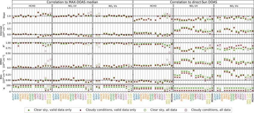
8                                                                         J.-L. Tirpitz et al.: CINDI-2 profiling comparison

2.2.3   NO2 profiles                                              mined by applying the so-called minimum Langley extrapo-
                                                                  lation (Herman et al., 2009). The temperature dependence of
NO2 profiles were recorded sporadically by two measure-           the NO2 cross sections was used to separate the tropospheric
ment systems: radiosondes (described in Sluis et al., 2010)       from the stratospheric column.
and an NO2 lidar (Berkhout et al., 2006). Radiosondes were           HCHO VCDs were retrieved from data of the BIRA
launched at the CESAR measurement site during the cam-            DOAS instrument (number 4). A fixed reference spectrum
paign. For this study, only data from sonde ascents through       acquired on 18 September 2016 at 09:41 UTC and 55.6◦
the lowest 4 km (which is the MAX-DOAS profiling retrieval        SZA was used. DOAS fitting settings were identical to those
altitude range) were used. A sonde profile was considered         used for the CINDI-2 HCHO dSCD intercomparison (Kreher
temporally coincident to a MAX-DOAS profile, when the             et al., 2019). The residual amount of HCHO in the reference
middle timestamps of MAX-DOAS elevation scan and sonde            spectrum of (8.8±1.6)×1015 molec. cm−2 was estimated us-
flight were less than 30 min apart. The horizontal sonde flight   ing a MAX-DOAS profile retrieved on the same day and a
paths are indicated in Fig. 1. Typical flight times (lowest       geometrical air mass factor (AMF) corresponding to 55.6◦
4 km) were of the order of 10–15 min. Data were recorded          SZA. Because of that, the HCHO VCDs cannot be consid-
at a rate of 1 Hz, typically resulting in a vertical resolution   ered as a fully independent dataset. VCDs were calculated
of approximately 10 m at an approximate measurement un-           from total HCHO slant column densities (SCDs) using a ge-
certainty in NO2 concentration of 5 × 10¹⁰ molec. cm−3 . The      ometrical AMF including a simple correction for the Earth’s
horizontal travel distances varied strongly between 4 and         sphericity. Only spectra with DOAS fit residuals < 5 × 10⁻⁴
18 km. A detailed overview of the flights is given in Sup-        were considered as valid direct-sun data. As for AOTs, these
plement Sect. S4.2.                                               observations can only be performed when the Sun is clearly
   The NO2 lidar is a mobile instrument setup inside a lorry      visible; hence, the coverage for cloudy scenarios is scarce.
which was located close to the CESAR meteorological tower.
It combines lidar observations at different viewing elevation     2.2.5   Trace gas surface concentrations
angles to enhance vertical resolution and to obtain sensitivity
close to the ground, despite the limited range of overlap be-     Note that in the following, “surface concentration” will not
tween sending and receiving telescope (see also Sect. 2.2.2).     refer to measurements in the very proximity to the ground but
The instrument is sensitive along its line of sight from 300      to the average concentration in the lowest 200 m of the atmo-
to 2500 m distance to the instrument. The azimuthal point-        sphere, as retrieved for the MAX-DOAS first profile layer.
ing was 265◦ with respect to the north, and the operational       Trace gas surface concentrations of HCHO and NO2 were
wavelength is 413.5 nm. Typical specified uncertainties in the    provided by a long-path DOAS system operated by IUP-
retrieved concentrations are around 2.5 × 10¹⁰ molec. cm−3 .      Heidelberg (LP-DOAS; see Pikelnaya et al., 2007; Pöhler
Profiles were provided at a temporal resolution of 28 min,        et al., 2010; Merten et al., 2011; Nasse et al., 2019). The LP-
each profile consisting of a series of (occasionally overlap-     DOAS system consists of a light-sending and receiving tele-
ping) altitude intervals with constant gas concentration. For     scope unit located at 3.8 km horizontal distance to a retro re-
an exemplary profile and details on its conversion to the         flecting mirror mounted at the top (207 m altitude) of the me-
MAX-DOAS retrieval altitude grid, please refer to Supple-         teorological tower (see Supplement Sect. S4.4). Light from a
ment Sect. S4.3. A lidar profile was considered temporally        UV–Vis light source is sent by the telescope to the retroreflec-
coincident to a MAX-DOAS profile, when the middle times-          tor and the reflected light is again received by the telescope
tamps of MAX-DOAS elevation scan and lidar profile were           unit and spectrally analysed applying the DOAS method. The
less than 30 min apart. This resulted in 25 suitable lidar pro-   fundamental difference to the MAX-DOAS instruments is
files recorded on six different days during the campaign. Ex-     the well-defined light path which enables very accurate de-
ample profiles of both radiosonde and NO2 lidar are shown         termination of trace gas mixing ratios, averaged along the
in the course of a comparison between the two observations        line of sight. Accordingly, with the retroreflector mounted at
in Supplement Sect. S4.5.                                         207 m altitude, one obtains average mixing ratios over the
                                                                  lowest MAX-DOAS retrieval layer, as indicated in Fig. 1.
2.2.4   Trace gas vertical column densities                       Considering DOAS fitting errors and uncertainties in the ap-
                                                                  plied literature cross sections (Vandaele et al., 1998; Meller
Tropospheric trace gas VCDs were derived from direct-sun          and Moortgat, 2000; Pinardi et al., 2013) yields an average
DOAS observations, which were performed between min-              accuracy of the LP-DOAS of ±1.5 × 10⁹ molec. cm−3 ± 3 %
utes 40 and 45 of each hour. NO2 VCDs were retrieved from         (± 5 × 10⁹ molec. cm−3 ± 9 %) for NO2 (HCHO), respec-
combined datasets of two Pandora DOAS instruments (in-            tively. Given the high accuracy, the total vertical coverage
strument numbers 31 and 32) and calculated based on the           of the surface layer and a near-continuous dataset over the
Spinei et al. (2014) approach. The reference spectrum was         campaign period, the LP-DOAS provides the most reliable
created from the spectra with lowest radiometric error over       dataset for the validation of CINDI-2 MAX-DOAS trace gas
the whole campaign and the residual NO2 signal was deter-         profiling results.

Atmos. Meas. Tech., 14, 1–35, 2021                                                     https://doi.org/10.5194/amt-14-1-2021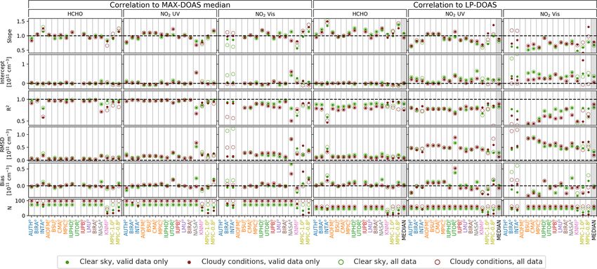
J.-L. Tirpitz et al.: CINDI-2 profiling comparison                                                                               9

   Further observations for qualitative validation are the sur-     ments. (iii) The real conditions encountered can exceed the
face values of the NO2 lidar and the radiosondes and also           model’s scope because horizontal inhomogeneities or the fact
in situ monitors in the CESAR meteorological tower. Tele-           that many of the fixed forward model input parameters (such
dyne in situ NO2 monitors (Teledyne API, model M200E)               as aerosol properties, surface albedo, temperature and pres-
were located in the tower basement and were subsequently            sure profiles) are averaged quantities of former observations
connected to different inlets located at 20, 60, 120 and 200 m      which might be inaccurate for specific days and conditions.
altitude (switching intervals approx. 5 min). Further, a CAPS       (iv) In some cases, different participants used the same re-
(type AS32M, based on attenuated phase shift spectroscopy,          trieval algorithms; this allows an assessment of the impact
Kebabian et al., 2005) and a CE-DOAS (cavity-enhanced               of different settings in the remaining parameters, which were
DOAS; Platt et al., 2009 and Horbanski et al., 2019) were           not prescribed (see Sect. 2.1.3). The approaches chosen here
continuously measuring at 27 m altitude. All the in situ mea-       are therefore limited to the examination of (i) the consis-
surements at the tower were combined to obtain another set          tency among the participants, (ii) the consistency of the re-
of surface concentration measurements, more representative          sults with available supporting observations and (iii) inherent
of concentrations close to the site. The data were combined         quality proxies of the retrieval (described in the next para-
by linearly interpolating over altitude between the instru-         graph). Table 4 summarizes the quantities which are com-
ments and subsequently averaging the resulting profile over         pared, together with the corresponding supporting observa-
the retrieval surface layer (0–200 m altitude). Note that this      tions if available.
method gives a large weight to the uppermost measurements,             In this study, agreement between different observations is
as they are representative of the majority of the relevant layer.   statistically assessed by (i) weighted RMSDs, (ii) weighted
                                                                    “bias” as introduced below and (iii) weighted least-squares
2.2.6    Meteorology                                                regression analysis. Discussions and summary are focused
                                                                    on RMSD, being the most fundamental quantity as it rep-
Meteorological data for the surface layer (pressure, temper-        resents both statistical and systematic deviations. The bias
ature and wind information) routinely measured at the CE-           was introduced as a general proxy for systematic deviations.
SAR site were taken from the CESAR database (CESAR,                 Correlation coefficient, slope and offset from the regression
2018) at a temporal resolution of 10 min. Cloud conditions          analysis are provided and consulted for a more differentiated
were retrieved from MAX-DOAS data of instruments 4 and              view.
28 according to the cloud classification algorithm developed           Consider two time series of length NT : the retrieval result
by MPIC (Wagner et al., 2014; Wang et al., 2015). Basically,        xp,t of a participant p at time t and some reference observa-
only two cloud condition states are distinguished in the statis-    tion xref,t (either MAX-DOAS median results or data from
tical evaluation: “clear-sky” (green) and “presence of clouds”      supporting observations, as further described below) with as-
(red). Only in the overview and correlation plots, “presence        sociated uncertainties σp,t and σref,t . Then the RMSD is de-
of clouds” is further subdivided into “optically thin clouds”       fined as
(orange) and “optically thick clouds” (red). According to this                          s
                                                                                            1      1      X                  2
classification, 72 (98) of the 170 profiles were measured un-       RMSD: σrms,p =             ·P       ·    wt xp,t − xref,t . (5)
der clear-sky (cloudy) conditions. Over the whole campaign,                                NT      t wt   t
there was only one rain event (precipitation > 0.01 mm) co-
                                                                    The weights wt are defined according to
inciding with the measurements on 25 September 2016 be-
tween 15:00 and 17:00 UT. At forenoon on 16 September, a                          1
                                                                    wt =    2         2
                                                                                                                               (6)
heavy fog event strongly limited the visibility (see also Sup-             σp,t   + σref,t
plement Sect. S5).
                                                                    and are also applied for the bias calculation and regression
2.3     Comparison strategy                                         analysis. The bias is defined as
                                                                                     1       1     X
2.3.1    General approach                                           bias: σbias,p =      ·P      ·    wt xp,t − xref,t .     (7)
                                                                                    NT        w
                                                                                             t t    t

Different MAX-DOAS retrieval algorithms were extensively            Sometimes, the term “average RMSD” (“average bias”) is
compared in Frieß et al. (2019) using synthetic data. The cru-      used, which refers to the average over the RMSD (bias) val-
cial differences of the presented study are that (i) the under-     ues of the individual participants. We further introduce the
lying spectra are not synthetic but were recorded with real         “average bias magnitude” that averages the absolute values
instruments, meaning that real noise and instrument arte-           of the bias. When referring to “relative RMSDs” (“relative
facts propagate into the results. (ii) Independent informa-         bias”), the underlying RMSD (bias) value was divided by the
tion on the real profile can only be inferred from support-         average of the investigated quantity. For the linear regression
ing observations with their own uncertainties and an imper-         analysis, the vertical distance between the model and the data
fect spatiotemporal overlap with the MAX-DOAS measure-              points is minimized and also here the weights wt are applied.

https://doi.org/10.5194/amt-14-1-2021                                                        Atmos. Meas. Tech., 14, 1–35, 2021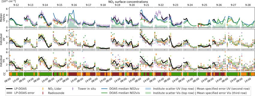
10                                                                                              J.-L. Tirpitz et al.: CINDI-2 profiling comparison

Table 4. Overview of compared quantities and available supporting data.

              Species             Quantity                                   Supporting observations                    Results section
              Aerosol UV          Profiles                                   Ceilometera (Sect. 2.2.2)                  3.2 and Supplement S8.2
                                  AOT                                        Sun photometer (Sect. 2.2.1)               3.4
              Aerosol Vis         Profiles                                   Ceilometera                                3.2 and Supplement S8.2
                                  AOT                                        Sun photometer                             3.4
              HCHO                Profiles                                   Not available                              3.2 and Supplement S8.2
                                  VCD                                        Direct-Sun DOAS (Sect. 2.2.4)              3.5
                                  Surface concentration                      Long-path DOAS                             3.6
              NO2 UV–Vis          Profiles                                   NO2 lidar and radiosondeb                  3.2 and Supplement S8.2
                                  VCD                                        Direct-Sun DOAS                            3.5
                                  Surface concentration                      Long-path DOAS                             3.6
              All species         Modelled vs. measured dSCDs                Not availablec                             3.3
            a Elastic backscatter profiles scaled with the Sun photometer or MAX-DOAS AOT. b Scarce data coverage. c Inherent quality proxy.

   To assess the consistency among the participants, the me-                          with x̄h,t being the average (over participants) MAX-DOAS
dian result over the valid profiles of all participants is inserted                   retrieved concentration for a given time t and layer h. If
as xref,t . The median is used instead of the mean value, since                       not stated otherwise, ASDev values of profiles are calculated
it is less sensitive to (sometimes unphysical) outliers. This                         considering the lowest five retrieval layers (up to 1 km alti-
comparison shows how far the choice of the retrieval algo-                            tude).
rithm or technique affects the results but it does not reveal                            In the statistical evaluations, clear-sky and cloudy condi-
general systematic MAX-DOAS retrieval errors. Outliers ob-                            tions as well as unfiltered and filtered data (according to the
served for distinct participants and algorithms are therefore                         flags provided by the participants) are distinguished. The dis-
not necessarily an indicator for poor performance.                                    tinction between cloud conditions is of major importance,
   To assess the consistency with supporting observations,                            as particularly in the case of aerosol retrievals under bro-
the latter are inserted as xref,t . This comparison is a bet-                         ken clouds, the quality of the results is typically strongly de-
ter indicator for the real retrieval performance. However,                            graded. A consequence of regarding these data subsets is that
uncertainties of supporting instruments (see Supplement                               the number of contributing data points not only depends on
Sect. S4.5), smoothing effects (see Sect. 2.3.2) and imper-                           the number of submitted profiles and the number of coinci-
fect spatial and temporal overlap of the different observations                       dent data points from supporting observations but further on
(see Sect. 2.3.3) complicate the interpretation.                                      the filter settings. Any regression RMSD or bias value with
   An inherent quality indicator for the retrieval algorithms                         less than five contributing data points is considered to be sta-
is the consistency of modelled and measured dSCDs. During                             tistically unrepresentative and is omitted. If not stated other-
the inversion, the goal is to minimize the deviation between                          wise, numbers given in the text were calculated considering
the RTM-simulated dSCDs and the actually measured ones.                               valid data only.
If strong deviations remain after the final iteration in the min-
imization process, this indicates failure of the retrieval.
                                                                                      2.3.2     Smoothing effects
   In a few cases (e.g. Sect. 3.2, where full profiles are com-
pared), the scatter among several participants p (of number
NP ) and several retrieval layers h (of number NH ) is of in-                         As shown in Sect. 3.1 below, in particular in the UV range,
terest. For this purpose, we define the “average standard de-                         the sensitivity of ground-based MAX-DOAS observations
viation” (ASDev) which is the standard deviation observed                             decreases rapidly with altitude, meaning that species above
among the participants for individual profiles averaged over                          ≈ 2 km typically cannot be reliably quantified. At higher al-
retrieval layers and time; hence,                                                     titudes, OEM retrieval results are drawn towards the a priori
                                                                                      profile (according to the definition of the cost function; see
                                                                                      Rodgers, 2000), while the results of parameterized and ana-
                    1 X                                                               lytical approaches are driven by the chosen parametrization
ASDev: σasdev =
                   NT t                                                               and their implementation. Further, the vertical resolution is
                       s                                                              limited (from 100 to several hundred metres, increasing with
                    1 X   1 X                  2                                     altitude), which affects the profile shape and – of most im-
                                 xp,h,t − x̄h,t ,                          (8)
                   NH h NP − 1 p                                                      portance in this study – the retrieved surface concentration.

Atmos. Meas. Tech., 14, 1–35, 2021                                                                                https://doi.org/10.5194/amt-14-1-2021
J.-L. Tirpitz et al.: CINDI-2 profiling comparison 11
Both effects cause deviations from the true profile that are in Spatial mismatches are of the order of 10 km; temporal mis-
the following referred to as “smoothing effects”. matches vary between 0 and 20 min. Consequently, strong
For a meaningful quantitative comparison, they should be spatiotemporal variations of the observed quantities are ex-
considered. This is possible for OEM retrievals, where the pected to induce large discrepancies among the observa-
information on the vertical resolution and sensitivity is given tions, independent of the data quality. Quantitative estimates
by the averaging kernel matrix (AVK; see Sect. 3.1 for de- of the impact on the comparison could only be derived for
tails). For a meaningful quantitative comparison of an OEM- NO2 surface concentrations and under strong simplifications
retrieved profile and a validation profile x (assumed here to (for details, see Supplement Sect. S6), yielding an RMSD
perfectly represent the true state of the atmosphere), the val- of 3.5 × 10¹⁰ molec. cm−3 . This is indeed of similar magni-
idation profile resolution and information content has to be tude as the average RMSD observed during the comparison
degraded by “smoothing” it with the corresponding MAX- (approx. 5 × 10¹⁰ molec. cm−3 ). It shall further be noted that
DOAS AVK matrix A according to the following equation under strong spatial variability the horizontal homogeneity
(Rodgers and Connor, 2003; Rodgers, 2000): assumed by the retrieval forward models is inaccurate.
x = Ax + (1 − A)x a .
e (9)
Here, x a is the a priori profile and e x represents the profile 3 Comparison results
that a MAX-DOAS OEM retrieval (with the resolution and
sensitivity described by A) would yield in the respective sce- 3.1 Information content
nario. For layers with high (low) gain in information, e x is
drawn towards x (x a ), while vertical resolution is degraded if In the case of OEM retrievals, the gain in information on
A has significant off-diagonal entries (compare to Sect. 3.1). the atmospheric state can be quantified according to Rodgers
In this study, this has implications not only for the compari- (2000). Essentially speaking, this is done by comparing the
son of profiles but also the comparison of the total columns knowledge before (represented by the a priori profile and its
(AOTs and VCDs, which are derived simply by vertical in- uncertainties) and after the profile retrieval. The gain in in-
tegration of the corresponding profiles) and surface trace gas formation for each individual vertical profile can be repre-
concentrations. For total columns, the dominant issue is the sented by the AVK matrix (denoted by A). Aij describes the
lack of information at higher altitudes. In contrast, there is sensitivity of the measured concentration in the ith layer to
reasonable information on the surface concentration; how- small changes in the real concentration in the j th layer. Each
ever, smoothing can have a severe impact here in the case row Ai can thus be plotted over altitude providing the fol-
of strong concentration gradients close to the surface. The lowing information: (1) the value in the layer i itself (the
impact on the individual observations is discussed in the cor- diagonal element Aii with a value between 0 and 1) gives the
responding sections below. A particularly important conse- gain in information while 1 − Aii represents the amount of
quence of smoothing effects is the “partial AOT correction” a priori knowledge which had to be assimilated to obtain a
(PAC), which is introduced and discussed in Sect. 3.4. well-defined concentration value. (2) The values in the other
Finally, it shall be pointed out that the sensitivity and spa- layers (off-diagonal elements of A) indicate the cross sen-
tial resolution are strongly affected by the exact approach sitivity of layer i to layer j . Typically, the cross sensitivity
that is chosen to solve the ill-posed inversion problem. Frieß decreases with the distance to the layer i. The length of this
et al. (2006), for instance, demonstrates that the sensitivity to decay (note that i can be converted to the corresponding alti-
higher altitudes can be enhanced by relaxing the prior con- tude by multiplication with the retrieval layer thickness 1h)
straints and by retrieving profiles at several wavelengths si- is an indicator for the vertical resolution of the retrieval. The
multaneously. trace of A is equal to the DOFS and hence the total number
of independent pieces of information gained from the mea-
2.3.3 Spatiotemporal variability surements compared to the a priori knowledge. Figure 2 vi-
sualizes the average AVK matrices (median over participants
It is obvious already from Fig. 1 and Sect. 2.2 that the and mean over time) for all five species studied in this work.
MAX-DOAS instruments and the various supporting obser- Note that the AVKs do not necessarily represent the real or
vations sample different air volumes at different times. In total sensitivity and information content of MAX-DOAS ob-
addition, the MAX-DOAS horizontal viewing distance (de- servations as they only consider the gain of information with
rived in Supplement Sect. S5) is highly variable, chang- respect to the a priori knowledge. Hence, for stricter a priori
ing between 2 and 30 km during the campaign for the low- constraints, less gain in information will be indicated by the
est viewing elevation angles. Similar investigations were al- AVKs.
ready performed by Irie et al. (2011) using CINDI-1 data; With the a priori profiles and covariances used within this
however, they used a different definition of the viewing dis- study, the sensitivity is limited to about the lowest 1.5 km
tance. Table S6 summarizes the spatial and temporal mis- of the atmosphere for all species. More information is ob-
matches between MAX-DOAS and supporting observations. tained on the Vis species, as the differential light path in-
https://doi.org/10.5194/amt-14-1-2021 Atmos. Meas. Tech., 14, 1–35, 202112 J.-L. Tirpitz et al.: CINDI-2 profiling comparison
Figure 2. Mean AVKs for the retrieved species (median over participants, mean over time). Their meaning is described in detail in the text.
Each altitude and corresponding AVK line Ai are associated with a colour, which is defined by the colour of the corresponding altitude-axis
label. The dots mark the AVK diagonal elements. The numbers next to the dots show the exact value in percent, which corresponds to the
amount of retrieved information on the respective layer. In each panel, the numbers indicate the DOFS (median among institutes, average
over time) for clear-sky (green) and cloudy conditions (red).
creases with wavelength resulting in higher sensitivity. The content, since the light paths are shorter and their geometry
obtained DOFS values are generally a bit lower as observed depends less on the viewing elevation.
in former studies. This is related to the rather small a pri-
ori covariance (50 %; see Sect. 2.1.3), which implies a good 3.2 Overview plots
knowledge on the atmospheric state prior to the retrieval and
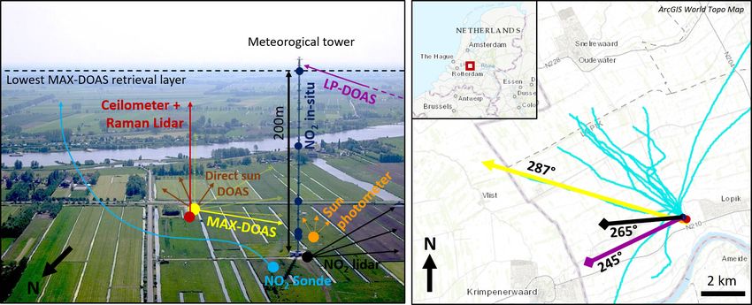
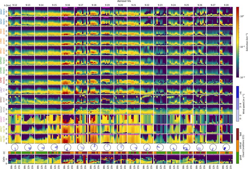
finally leads to less gain in information from the measure- Figures 3 to 7 show the retrieved profiles of all participants
ments. Figures S35, S36, S37, S38 and S39 in Supplement over the whole semi-blind period. They serve as the basis
Sect. S8.1 show the average AVKs of the individual partici- for a general qualitative comparison. For the trace gases, the
pants and reveal that there are significant differences (up to altitude ranges (full range is 4 km) were reduced to 0–2.5 km
1 DOFS) between the participants even when using the same for better visibility, considering the MAX-DOAS sensitivity
algorithm (up to 0.5 DOFS in the case of PriAM). This in- range and the occurrence altitude of the respective species.
dicates that the information content is not assessed consis- Considering valid data only, all algorithms detect simi-
tently. BOREAS, for instance, states a very low gain in in- lar features in the vertical profiles but smoothed to differ-
formation especially for aerosol Vis. This is related to an ad- ent amounts and sometimes detected at different altitudes.
ditional Tikhonov term used as a smoother which was also For clear-sky conditions, the observed ASDevs are 3.5 ×
applied during AVK assessment. Furthermore, all BOREAS 10−2 km−1 for aerosol UV, 4.0 × 10⁻² km−1 for aerosol Vis,
results were retrieved on another grid and interpolated onto 1.2 × 10¹⁰ molec. cm−3 for HCHO, 2.4 × 10¹⁰ molec. cm−3
the submission grid, which leads to a decrease in all AVKs for NO2 UV and 4.4 × 10¹⁰ molec. cm−3 NO2 Vis. When re-
and therefore the DOFS. On average, the dependence of the garding participants using the same algorithm, these values
total amount of information on the cloud conditions is small are reduced only by about 50 %, indicating that significant
(typically decrease of 0.1 DOFS). Examination of the AVKs discrepancies are caused by differences in the user-defined
of individual profiles (not shown here), indicated that there retrieval settings that were not prescribed. The latter are, for
are two competing effects: (1) the presence of clouds can in- instance, the accuracy criteria for the RTMs, the number of
crease the sensitivity to higher layers due to multiple scatter- iterations in the inversion, the convergence criteria or the de-
ing and thus light path enhancement in the clouds, whereas cision at which points of the iteration process the forward
(2) a decrease in the horizontal viewing distance (e.g. due model Jacobians are (re)calculated. An example are the dis-
to fog, rain or high aerosol loads) reduces the information crepancies between UTOR/HEIPRO and IUPHD/HEIPRO.
In this case, the number of applied iteration steps in the
aerosol inversion was identified as the main reason: UTOR
Atmos. Meas. Tech., 14, 1–35, 2021 https://doi.org/10.5194/amt-14-1-2021You can also read