GreenHouse gas Observations of the Stratosphere and Troposphere (GHOST): an airborne shortwave-infrared spectrometer for remote sensing of ...
←
→
Page content transcription
If your browser does not render page correctly, please read the page content below
Atmos. Meas. Tech., 11, 5199–5222, 2018
https://doi.org/10.5194/amt-11-5199-2018
© Author(s) 2018. This work is distributed under
the Creative Commons Attribution 4.0 License.

GreenHouse gas Observations of the Stratosphere and Troposphere
(GHOST): an airborne shortwave-infrared spectrometer for remote
sensing of greenhouse gases
Neil Humpage1 , Hartmut Boesch1,2 , Paul I. Palmer3,4 , Andy Vick5,a , Phil Parr-Burman5 , Martyn Wells5 ,
David Pearson5 , Jonathan Strachan5 , and Naidu Bezawada5,b
1 EarthObservation Science, Department of Physics and Astronomy, University of Leicester, Leicester, UK
2 National Centre for Earth Observation, Leicester, UK
3 School of GeoSciences, University of Edinburgh, Edinburgh, UK
4 National Centre for Earth Observation, Edinburgh, UK
5 Science and Technology Facilities Council, UK Astronomy Technology Centre, Edinburgh, UK
a now at: Science and Technology Facilities Council, Rutherford Appleton Laboratory, Harwell, Oxfordshire, UK
b now at: European Southern Observatory, Garching, Germany

Correspondence: Neil Humpage (nh58@le.ac.uk)

Received: 21 December 2017 – Discussion started: 10 January 2018
Revised: 1 August 2018 – Accepted: 16 August 2018 – Published: 12 September 2018

Abstract. GHOST is a novel, compact shortwave-infrared            over the ocean, where ground-based validation measure-
grating spectrometer, designed for remote sensing of tropo-       ments are not available. In this paper we provide an overview
spheric columns of greenhouse gases (GHGs) from an air-           of the GHOST instrument, calibration, and data processing,
borne platform. It observes solar radiation at medium to high     demonstrating the instrument’s performance and suitability
spectral resolution (better than 0.3 nm), which has been re-      for GHG remote sensing. We also report on the first GHG ob-
flected by the Earth’s surface using similar methods to those     servations made by GHOST during its maiden science flights
used by polar-orbiting satellites such as the JAXA GOSAT          on board the NASA Global Hawk unmanned aerial vehicle,
mission, NASA’s OCO-2, and the Copernicus Sentinel-5 Pre-         which took place over the eastern Pacific Ocean in March
cursor. By using an original design comprising optical fibre      2015 as part of the CAST/ATTREX joint Global Hawk flight
inputs along with a single diffraction grating and detector ar-   campaign.
ray, GHOST is able to observe CO2 absorption bands cen-
tred around 1.61 and 2.06 µm (the same wavelength regions
used by OCO-2 and GOSAT) whilst simultaneously measur-
ing CH4 absorption at 1.65 µm (also observed by GOSAT)            1   Introduction
and CH4 and CO at 2.30 µm (observed by Sentinel-5P). With
emissions expected to become more concentrated towards            The Paris Agreement (2015) describes a framework for mit-
city sources as the global population residing in urban ar-       igating global anthropogenic greenhouse gas (GHG) emis-
eas increases, there emerges a clear requirement to bridge the    sions. The success of this agreement lies in our ability
spatial scale gap between small-scale urban emission sources      to monitor progress on nationally determined contributions
and global-scale GHG variations. In addition to the bene-         (NDCs) that describe country emission targets (Article 13 of
fits achieved in spatial coverage through being able to re-       the Paris Agreement). This will be achieved by global stock
motely sense GHG tropospheric columns from an aircraft,           takes every 5 years from 2023 (Article 14). The Paris Agree-
the overlapping spectral ranges and comparable spectral res-      ment emphasizes, in particular, the requirement of indepen-
olutions mean that GHOST has unique potential for provid-         dent verification of emissions or monitoring independent
ing validation opportunities for these platforms, particularly    data. One approach to independently assessing GHG emis-

Published by Copernicus Publications on behalf of the European Geosciences Union.
5200           N. Humpage et al.: An airborne shortwave-infrared spectrometer for remote sensing of greenhouse gases

sions is to monitor atmospheric concentrations of GHGs. At-        ject to clouds and elevated aerosol loading, but at exclusively
mospheric GHGs vary over a range of temporal and spa-              one local time of the day with a typical repeat frequency of
tial scales, reflecting variations due to their sources, sinks,    a few days. The integrated column measurement can help to
and atmospheric transport. Here, we describe the calibration       overcome these weaknesses: a column measurement at any
and performance of a new airborne remote-sensing GHG in-           one time and location is a superposition of sources and sinks
strument that seeks to fill the spatial measurement gap be-        from upwind regions at different times of day (Palmer et al.,
tween ground-based remote-sensing instruments and satellite        2008). This does, however, make interpretation of the col-
data. Data from this airborne instrument have the potential        umn non-trivial, and consequently it would be difficult with
to link emissions from small-scale (< 1 km) sources to the         current measurement techniques, even if properly integrated
global-scale atmospheric GHG variations that are currently         through intercalibration efforts, to address the objectives of
observed by both ground-based networks and satellite instru-       the Paris Agreement given the importance of city and point
ments.                                                             emission sources.
   A large number of atmospheric GHG measurements are                 Aircraft remote-sensing instruments are particularly well
collected daily across the globe. Each type of atmospheric         suited for mapping out small-scale gradients in GHGs, en-
GHG measurement has its advantages and disadvantages.              abling repeated observations over large point sources and dif-
Global-scale in situ measurement networks were designed to         fuse sources and providing a link between ground-based in
precisely and accurately observe large-scale changes in at-        situ measurements and space-borne observations. The Air-
mospheric GHGs (e.g. NOAA ESRL, https://www.esrl.noaa.             borne Research Interferometer Evaluation System (ARIES)
gov/, last access: 29 August 2018). They provide invaluable        is a Fourier transform spectrometer (FTS), which is regularly
information on baseline values, and records are typically col-     flown on the UK FAAM (Facility for Airborne Atmospheric
lected over many decades. These have recently been supple-         Measurements) BAe-146 atmospheric research aircraft. Re-
mented by smaller, denser networks within individual coun-         cent work has developed the capability to retrieve thermal in-
tries (Henne et al., 2016; Palmer et al., 2018) and in some        frared (TIR) CH4 columns that have helped to map distribu-
cases within individual cities whose purpose is to quantify        tions of CH4 gradients over the UK (Illingworth et al., 2014;
national, regional, and local GHG emissions (Bréon et al.,         Allen et al., 2014). The German Methane Airborne MAPper
2015; Davis et al., 2017). Similar in situ instruments are         (MAMAP) is a two-channel near- and/or shortwave-infrared
installed on atmospheric research aircraft (Pitt et al., 2016;     (NIR/SWIR) grating spectrometer (Gerilowski et al., 2011;
O’Shea et al., 2013) and in some instances commercial air-         Krings et al., 2011) that was designed to fly on a range of
craft (Brenninkmeijer et al., 2007; Matsueda et al., 2002).        aircraft. MAMAP has illustrated the usefulness of airborne
These measurement platforms allow the study of vertical gra-       technology to map CH4 and CO2 emissions from coal mines,
dients but are typically deployed for short durations or over      landfill sites, and a North Sea bubble blow-out plume (Krings
limited spatial domains, although there are notable excep-         et al., 2013; Krautwurst et al., 2017; Gerilowski et al., 2015).
tions. Data collected by commercial aircraft represent valu-       CHARM-F (CO2 and CH4 Remote Monitoring-Flugzeug)
able knowledge of variations in the upper troposphere along        is an integrated-path differential-absorption lidar (Amediek
air corridors but also provide vertical profiles during air-       et al., 2017) that serves as the airborne demonstrator for
port ascents and descents. In addition to these in situ ob-        the DLR-CNES MERLIN (Methane Remote Sensing Lidar
servations, temporary networks of portable upward-looking          Mission) concept. CHARM-F simultaneously measures CO2
Fourier transform spectrometers (Gisi et al., 2012) have been      and CH4 columns and has flown on the German HALO
used to constrain GHG emissions on a local scale by making         (High Altitude and Long Range Research Aircraft). The po-
integrated column measurements of GHGs from different lo-          tential for using airborne hyperspectral imagers such as the
cations around a city (Hase et al., 2015; Viatte et al., 2017).    NASA Airborne Visible-Infrared Spectrometer – Next Gen-
   Satellite column observations of CO2 and CH4 with the           eration (AVIRIS-NG) to detect and quantify localized an-
precision necessary to determine their surface emissions are       thropogenic sources of CH4 has also been demonstrated re-
now available (Crisp et al., 2017; Kuze et al., 2009; Buchwitz     cently (Thompson et al., 2015). A further NASA instrument,
et al., 2015; Feng et al., 2017). Because of the stringent mea-    called CARVE-FTS (Carbon in Arctic Reservoirs Vulner-
surement requirements (precisions of < 1 ppm for CO2 and           ability Experiment FTS), has been used to observe GHG
< 5 ppb for CH4 ) reflecting the small fractional variations in-   fluxes from an aircraft over Alaska (Dupont et al., 2012).
troduced by surface sources and sinks, systematic errors of a         In this paper we describe the GreenHouse gas Ob-
few percent in the column amount can, if not properly char-        servations of the Stratosphere and Troposphere (GHOST)
acterized, compromise the usefulness of the inferred GHG           shortwave-infrared (SWIR) grating spectrometer. The prin-
fluxes (Chevallier et al., 2014; Feng et al., 2016). To help       cipal advantage of the GHOST design (described in Sect. 2)
characterize these errors a global intercalibrated network of      is that it is able to image four different spectral bands using
upward-looking Fourier transform spectrometers has been            a single diffraction grating and detector array, thus saving on
established to validate the space-borne data (Wunch et al.,        space and weight compared with an equivalent instrument
2011). Nevertheless these data provide global coverage, sub-       using a separate grating and detector for each band. This ex-

Atmos. Meas. Tech., 11, 5199–5222, 2018                                              www.atmos-meas-tech.net/11/5199/2018/
N. Humpage et al.: An airborne shortwave-infrared spectrometer for remote sensing of greenhouse gases 5201
tent of wavelength coverage at high spectral resolution, and
subsequently the number of different gases that can be ob-
served, is unique for an airborne remote sensing instrument.
As well as the instrument design we also show the first set
of results from GHOST science flights on board the NASA
Global Hawk, which took place during the CAST-ATTREX
flight campaign, and describe the methods behind their pro-
duction from raw GHOST data. Section 3 describes the lab-
oratory measurements used to perform radiometric and spec-
tral calibration on GHOST and assesses its performance. In
Sect. 4 we outline the involvement of GHOST in CAST-
ATTREX, which was based at NASA Armstrong in Califor-
nia during early 2015. Finally, we present the first GHOST
flight results (along with the optimal estimation method used
to retrieve them from the calibrated radiance spectra) in
Sect. 5 and summarize the paper in Sect. 6.
2 The GHOST instrument
The optical design behind GHOST was developed by the
STFC (Science and Technology Facilities Council) Astron-
omy Technology Centre during two design studies, both
funded by the UK Centre for Earth Observation Instrumenta-
tion (http://ceoi.ac.uk/, last access: 29 August 2018), which
demonstrated reductions in size and weight of SWIR Earth
observation spectrometers by using technology originally de-
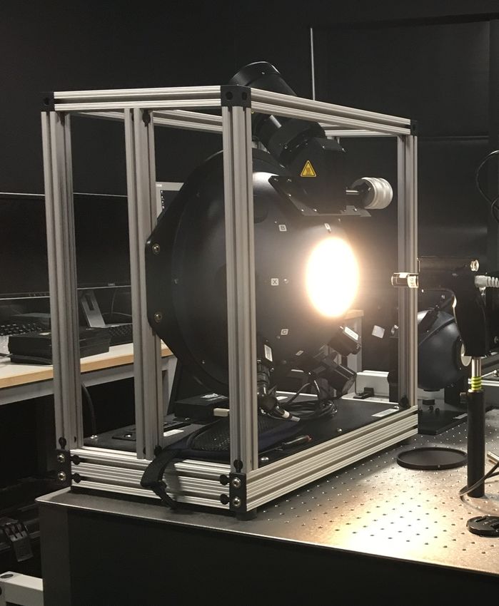
veloped for astronomy instruments. The optics use a combi- Figure 1. (a) Layout of the three main GHOST components
nation of blocking filters and multiple grating orders to pro- mounted in the lower instrument bay of the NASA Global Hawk.
vide spectra from several high-resolution bands from across a (b) Photograph taken from below showing the GHOST installation
wide range of wavelengths. As well as the size and weight ad- on the Global Hawk.
vantages, the optical fibre feed to the spectrometer provides
flexibility in the mechanical layout of the subsystems on dif-
ferent aircraft, thermo-mechanical isolation, and the possi- 2.1 The target acquisition module (TAM)
bility of optically isolated calibration light input to the spec-
The function of the TAM is to direct sunlight which has
trometer.
passed down through the atmosphere and then been reflected
The GHOST instrument, initially designed to meet the
back upwards by the Earth’s surface, onto an optical fibre
strict engineering requirements for installation on the NASA
bundle which transfers the light into the spectrometer mod-
Global Hawk unmanned aerial vehicle (UAV), takes advan-
ule. To achieve this, the TAM has to be able to acquire light
tage of an optical fibre feed system to split the optics into two
from any angle of rotation and up to 70◦ away from nadir,
units: the target acquisition module (TAM) and the spectrom-
depending on the solar zenith angle. A custom off-axis tele-
eter module. Figure 1 shows how these two components were
scope arrangement is used and mounted to a custom New-
mounted on a pallet on the underside of the Global Hawk,
mark GM-6 gimbal (see Fig. 3).
along with the air transport rack (ATR), which houses the
A fold mirror reflects the light path along the elevation
electronics and support equipment for the instrument. In this
axis of the gimbal, through a depolarizing unit and onto a
section we discuss each of these three components in turn. A
second fold mirror that directs the light path along the ro-
block diagram showing an overview of how the three com-
tation axis (see Fig. 4). Mounted centrally along this axis
ponents work together within the GHOST instrument system
are the pre-fibre optics (a field stop and lenses) and the fi-
is given in Fig. 2.
bre bundle mounting point. A field stop of diameter 2.6 mm
is used to define the range of angles from which light will
be accepted into the fibres, such that it observes reflected
light from a surface footprint 1◦ in diameter. The optics cre-
ate a pupil image on the end of the fibre bundle such that
the light is both concentrated onto the fibres and evenly dis-
tributed between them. The field stop defines the range of
www.atmos-meas-tech.net/11/5199/2018/ Atmos. Meas. Tech., 11, 5199–5222, 2018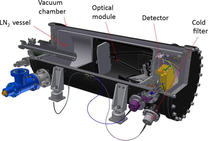
5202            N. Humpage et al.: An airborne shortwave-infrared spectrometer for remote sensing of greenhouse gases

Figure 2. Block diagram showing the three main components of the GHOST instrument (described in Sect. 2) and how they interact with
one another.

                                                                      is used to help interpret the science data, e.g. by identifying
                                                                      when the spectrometer field of view is cloud-free.
                                                                         The light enters the TAM through a dome whose centre of
                                                                      curvature has been placed at the centre of curvature of the
                                                                      gimbal to reduce differential aberrations across the gimbal
                                                                      range. Originally the whole bottom face of the TAM vessel
                                                                      was designed to be external to the aircraft, since the vessel
                                                                      was intended as an environmentally benign environment for
                                                                      the gimbal and the optics, with internal heaters and the po-
                                                                      tential for dry gas flushing. The TAM is pressurized to 3 psi
                                                                      above local ambient conditions to minimize the diffusion of
                                                                      water vapour into the optical system. The vessel also in-
                                                                      cluded a number of fiducial measurement points which were
                                                                      used to ascertain alignment and location of the optics, both
                                                                      in the lab and on the aircraft. The final installation was more
Figure 3. Cut-away model of the TAM showing the gimbal, pay-          enclosed and left only the dome itself protruding from the
load, and the edge of the dome (in dark blue). The light-blue com-    underside of the Global Hawk.
ponent rotates about the azimuthal axis, whilst the yellow compo-        The optical fibre bundle which passes the received light
nent rotates about the axis of elevation. The TAM is 513 mm tall      onto the spectrometer module is made up of 35 multimode
including the legs and has a diameter of 555 mm including the feet.   fibres, each with a 0.365 mm core, encased in a stainless steel
                                                                      outer sheath for protection. At the spectrometer end the bun-
                                                                      dle of 35 fibres is split into five smaller bundles (one for each
                                                                      spectral band; see Sect. 2.2) comprising seven fibres each,
angles that will be accepted into the fibres, which is set to an      with the choice of fibres kept as spatially random as possi-
angle of ± 6.67◦ (numerical aperture NA = 0.11). In order to          ble to ensure that a similar sampling of the aperture is passed
avoid misalignment between the main optical ray defined by            into each bundle. The light from each of the bundles is trans-
these apertures and the mechanical axis of the gimbal (which          mitted into the (cold) spectrometer through a window and
would introduce a shift in pointing angle which varies with           an order-sorting filter, which minimizes the out-of-band light
gimbal position), we required that the end of the fibre bundle,       and is finally coupled into a cold fibre bundle.
the coupling lens, and the field stop aperture should be cen-
tred on the rotation axis of the gimbal to within 50 µm. In the       2.2   The spectrometer module
focus direction (along the optical axis), they should be posi-
tioned to within an accuracy of 200 µm. The intersection of           Inside the spectrometer module there are three major sec-
the two mechanical axes of the gimbal must lie within 50 µm           tions: an end section that contains the optical entry points,
of the surface of fold mirror 2 (see Fig. 4), whilst the angle        cold fibres, and the detector box; a middle section contain-
of this mirror must also be correct to within 0.1◦ .                  ing the spectrometer optics; and a section where the cryogen
   By using a design which employs movable optics to trans-           tank is situated (see Fig. 5). All of the spectrometer module
fer the observed light onto a static fibre bundle, we minimize        internal components are cooled to 80 K, which has the effect
the potential for deterioration of the measured signal caused         of reducing the thermal background, the dark current on the
by movement and bending of the fibres. The gimbal also car-           detector, and any thermo-mechanical instabilities. The deci-
ries a wide-field panchromatic camera with a field of view            sion to use liquid nitrogen for cooling rather than a closed
extending beyond that of the spectrometer input. The camera           cycle cooler is based primarily on the need to minimize vi-

Atmos. Meas. Tech., 11, 5199–5222, 2018                                                 www.atmos-meas-tech.net/11/5199/2018/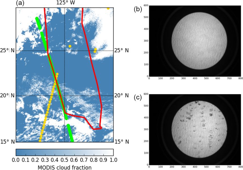
N. Humpage et al.: An airborne shortwave-infrared spectrometer for remote sensing of greenhouse gases                            5203

Figure 4. Optical path diagram showing how the optical components of the TAM direct the observed light into the optical fibre.

                                                                       of the curved camera mirror. The collimated beam is then
                                                                       reflected again by the fold mirror onto the grating, which
                                                                       disperses the light from each band into a number of spec-
                                                                       trally resolved images, each produced by a different order
                                                                       of diffraction. The dispersed light is reflected again by the
                                                                       fold mirror on to the other side of the camera mirror, af-
                                                                       ter which the converging beam is reflected once more by
                                                                       the fold mirror and passed through cylindrical output lenses
                                                                       that concentrate the spectral images onto the detector. The
                                                                       major innovation in this design is the use of multiple grat-
                                                                       ing orders: through the choice of orders and positioning of
                                                                       the input slits, multiple high-resolution spectral bands can be
                                                                       selected from a wide overall wavelength range and conve-
                                                                       niently placed onto the output plane. In the GHOST spec-
Figure 5. GHOST spectrometer module showing the front end com-
                                                                       trometer we use a 60 grooves mm−1 blazed grating supplied
partment, the main spectrometer optics area, and the liquid nitro-     by Richardson Gratings, with a blaze angle of 28.7◦ corre-
gen cryogenic vessel. The cylinder containing these components is      sponding to a blaze wavelength of 16 µm. For spectral bands
1064 mm long and 440 mm in diameter. Taking into account the fit-      1 through to 4 (Table 1) we use diffraction orders 13, 10, 8,
tings external to the cylinder, the space occupied is 1406 mm long,    and 7. The grating and orders were chosen to minimize the
758 mm wide, and 440 mm tall.                                          spread of input slit offsets (along the dispersion direction at
                                                                       the entrance to the spectrometer) required to image all of the
                                                                       bands onto the detector, using Band 2 as the reference point.
brations, both for this instrument and for other instruments           The spread was calculated for diffraction orders up to 18,
mounted on the same aircraft. Cryogenic cooling has the ad-            with the result that using diffraction order n = 10 for Band 2
ditional benefits of requiring no electrical power, being very         minimized the need to shift the input slits for the other bands.
reliable (compared with using mechanical cooling which re-             We then selected an appropriate grating by requiring that the
lies on moving components), and using little extra space for           blaze wavelength be as close to nλ for Band 2 as possible.
external electronics.                                                     The spectral images are recorded by a mercury cadmium
   We summarize the spectrometer optical design schemati-              telluride (MCT) detector, which is mounted just behind the
cally in Fig. 6. Observed light is brought into the spectrome-         optics baseplate. The detector used is a Raytheon Vision
ter optics using cold fibre bundles as mentioned in Sect. 2.1.         Systems VIRGO2K detector with 2048 × 2048 20 µm pix-
The optical part of the spectrometer module comprises four             els, which has high quantum efficiency (typically greater than
major components: the inlet slits, fold mirror, camera mir-            80 % across the broad spectral range), low dark current, and
ror, and grating (see Fig. 7). The f/5 focused beam from               low read noise (less than 20 e rms in a correlated double sam-
the input slits is reflected by the fold mirror onto one side          ple frame). The measured dark current at liquid nitrogen tem-

www.atmos-meas-tech.net/11/5199/2018/                                                     Atmos. Meas. Tech., 11, 5199–5222, 2018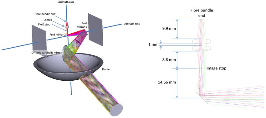
5204           N. Humpage et al.: An airborne shortwave-infrared spectrometer for remote sensing of greenhouse gases

Table 1. Target gases, spectral range, spectral resolution, and signal-to-noise ratio (SNR) design requirements for each band. The goal
(threshold in brackets) values are given for resolution and SNR. The SNR requirements listed here assume an integration time of 1 sec.

                      Band     Target gases                  Spectral range (µm)    Resolution (nm)         SNR
                      1        O2                            1.25–1.29                     0.1 (0.1)   200 (150)
                      2        CH4 , CO2                     1.59–1.675                   0.25 (0.3)    100 (80)
                      3        CO2                           2.04–2.095                   0.15 (0.3)   150 (100)
                      4        CO, CH4 , H2 O / HDO ratio    2.305–2.385                  0.25 (0.3)    100 (80)

Figure 6. Block diagram showing a simple overview of the GHOST
spectrometer optical layout.

perature (80 K) is less than 1 e s−1 pixel−1 . During flight we
use heaters and a platinum resistor (for feedback) to hold the
detector temperature at a slightly warmer 98 K, ensuring that         Figure 7. Elevation and plan view of the spectrometer showing the
the detector temperature remains stable to within a few tens          major dimensions, which allows it to fit into the cryostat optical
of mK via the feedback mechanism (the increased stability             module as shown in Fig. 5. The different coloured ray traces in the
is achieved in this way at the expense of a higher dark cur-          plan view diagram correspond to light from each of the five optical
rent; see Sect. 3.2). Prior to installation of the detector array     fibre bundles.
into the spectrometer module, we measured the average sig-
nal gain for each pixel to be 4.26 e count−1 .
   The spectrometer has been designed to measure high-                dancy in case the original Band 2 did not meet the spectral
resolution spectral radiances over four wavelength bands,             and radiometric requirements.
which we have chosen to coincide with spectral absorption
features of the atmospheric gases we are interested in. The           2.3   Data handling and control
design requirements for the four bands are listed in Table 1,
whilst Fig. 8 shows the absorption spectra of the most im-            The detector read-out system is an ARC (Astronomical Re-
portant gases in each band. When defining the requirements            search Camera) controller attached to an industrial PC run-
for the spectral resolution and signal-to-noise ratio we deter-       ning Linux. The software system is the UK-ATC’s UCam
mined threshold values, which indicate the minimum accept-            product, which has been widely used with astronomy instru-
able performance, along with goal values which represent the          ments across the world for the last 10 years. The detector
desired performance level. In the final design a fifth band, a        operates in an “integrate while read” mode, a non-destructive
duplicate of Band 2 (the most important band for meeting              read-out mode in which pixels can be sampled as many times
our science objectives), was incorporated to provide redun-           as required whilst integrating the signal. At 300 kHz pixel

Atmos. Meas. Tech., 11, 5199–5222, 2018                                                  www.atmos-meas-tech.net/11/5199/2018/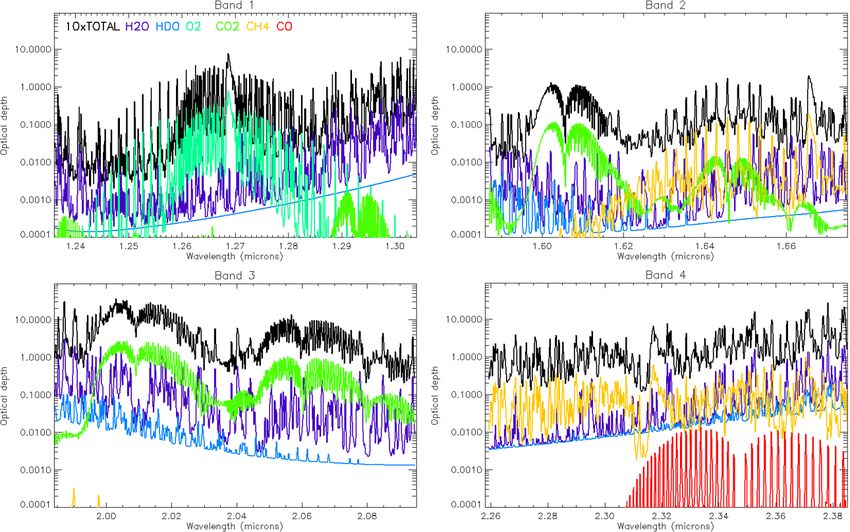
N. Humpage et al.: An airborne shortwave-infrared spectrometer for remote sensing of greenhouse gases                                 5205

Figure 8. Optical depth spectra for each of the four GHOST spectral bands listed in Table 1, calculated assuming a midlatitude reference
atmosphere and a viewing angle of 20◦ off nadir. The different colours correspond to the contributions towards the total optical depth from
each species considered. The total optical depth spectrum for each band (shown in black) is multiplied by 10 to make it easier to see on the
logarithmic scale.

rate, using all 16 amplifier channels, it takes about 0.91 s to         sured that the system would continue taking meaningful data
read out the entire detector. Since we are only imaging a frac-         under almost all conditions and, for extreme eventuality, pro-
tion of the array, we reduce the read-out time by skipping the          vided a hard reboot facility.
rows we do not need. By reading out only 300 of the 2048
detector rows (60 rows for each of the five bands), we reduce
the read-out time to 0.115 s. In order to maximize the on-              3   Calibration and performance of GHOST
source integration time, an up-the-ramp read-out mode has
been implemented where the array is read out a set number               In this section, we describe the procedures and measure-
of times following a reset (see Fig. 9). Both the number of             ments used for the radiometric and spectral calibration of
read-outs between resets and the dwell time between read-               the GHOST instrument, and provide a summary of the spec-
outs are programmable, and we set them such that the signal             trometer performance based on the calibration results. We
level prior to a reset is below the level at which the detec-           perform the majority of the calibration measurements using
tor is saturated. Taking the difference between any two reads           a 0.3 m internal diameter integrating sphere with 0.1 m di-
results in a frame which is free from the reset noise and the           ameter output port from Labsphere (Fig. 10), provided by
offset.                                                                 the NERC Field Spectroscopy Facility (FSF). The integrating
   The electronics for the read-out system are contained in             sphere produces a spatially uniform light source via multiple
the ATR, procured from Elma Electronic in the UK, which                 internal reflections off the inner Spectraflect coating, which
provides a temperature- and pressure-controlled environ-                completely illuminates the GHOST field of view when po-
ment. All data from the system (science data frames, aux-               sitioned at a distance of 1 m from the TAM. The integrat-
iliary pictures, temperatures, positional information, etc.) are        ing sphere used has four input ports in addition to the out-
stored on a solid-state disk in time-tagged netCDF files. The           put port: three ports housing quartz tungsten halogen (QTH)
system provides TCP (Transmission Control Protocol) and                 lamps (two internal to the sphere and one external), and one
UDP (User Datagram Protocol) command and control access                 port allowing the use of alternative light sources (such as the
via a 100BASE-T port as well as real time data access (over             emission lamps used for spectral calibration, as described in
TCP only). The software system is designed with robustness              Sect. 3.3) with the sphere. The two internal QTH lamps have
in mind, and a long campaign of simulated operations en-                output powers of 35 and 75 W, whilst the 150 W external

www.atmos-meas-tech.net/11/5199/2018/                                                      Atmos. Meas. Tech., 11, 5199–5222, 2018
5206            N. Humpage et al.: An airborne shortwave-infrared spectrometer for remote sensing of greenhouse gases

Figure 9. The sampling scheme used by the GHOST detector,
where we sample the array “up-the-ramp”. In this example we show
three reads of the array subset per exposure. Time treset = 0.115 s
is required to perform a destructive read-out and reset of the array
subset. A non-destructive read-out is then performed every tdwell
seconds. The number of reads and their duration are determined by      Figure 11. Diagram illustrating the steps and inputs involved dur-
the instrument operator.                                               ing the processing of GHOST data into calibrated radiance spectra.
                                                                       The numbers in bold contained in each of the inputs refer to the
                                                                       corresponding section number.

                                                                       for use in retrieval algorithms used to obtain concentrations
                                                                       of target trace gases (as described in Sect. 5.1). We summa-
                                                                       rize these steps in Fig. 11. The ellipses in the diagram indi-
                                                                       cate the inputs required, which we obtain during the instru-
                                                                       ment characterization and calibration described later in this
                                                                       section, whilst the rectangles show each separate processing
                                                                       step in the procedure. The raw detector frames at the start of
                                                                       the process are obtained by taking the final non-destructive
                                                                       read-out in a sequence and then subtracting the first read-out
                                                                       after the previous reset (see Fig. 9). The difference between
                                                                       these two read-outs removes the offset and reset noise as de-
                                                                       scribed in Sect. 2.3.

                                                                       3.2   Dark current measurement and identification
                                                                             of inactive pixels
Figure 10. Photograph of the NERC FSF integrating sphere, with
the 150 W external lamp and variable aperture mechanism visible
just above the output port (photograph by Chris MacLellan, NERC
                                                                       Prior to the spectral and radiometric calibration measure-
FSF).                                                                  ments, we need to characterize certain aspects of the detector
                                                                       array performance. These include the detector dark current
                                                                       (for each pixel on the array), the identification of the pix-
QTH lamp is mounted behind a mechanical variable aper-                 els that are illuminated on the detector array by each spec-
ture which allows fine adjustment of the output luminance.             tral band image, and the location on the array of dead, hot,
We use measurements of the 150 W external lamp for the                 or otherwise faulty pixels which are excluded from further
radiometric calibration described in Sect. 3.5. An internally          analysis.
mounted photodiode provides measurements of the output                    We evaluate the dark current (the residual current which
luminance at a frequency of 1 Hz.                                      flows through a photosensitive device in the absence of in-
                                                                       cident photons) by averaging over exposures taken with no
3.1    Processing of GHOST measurements into                           light entering the system, resulting in a dark current map in
       radiance spectra                                                units of digital counts per second. The mean dark current
                                                                       measured in each band is listed in Table 2. These values are
A number of steps are required to process the raw detector             higher than the 0.25 counts s−1 that would be achieved if the
frame data measured by GHOST into radiometrically and                  detector were operated at liquid nitrogen temperature (80 K;
spectrally calibrated radiance spectra, which are then suitable        see Sect. 2.2). However, we consider it more advantageous to

Atmos. Meas. Tech., 11, 5199–5222, 2018                                                   www.atmos-meas-tech.net/11/5199/2018/
N. Humpage et al.: An airborne shortwave-infrared spectrometer for remote sensing of greenhouse gases                               5207

Table 2. Mean dark current measured for each GHOST spectral            Table 3. Measurements used for the spectral calibration of GHOST
band (see Sect. 3.2) with the detector at flight temperature (98 K).   (see text in Sect. 3.3).
The standard deviations given represent the spatial variability of
dark current within each band.                                           Measurement                  Exposures   Reads per   Dwell per
                                                                                                                   exposure   read (ms)
         Band    Mean dark current     Standard deviation
                                                                         Argon pen-style lamp              100          12      10 000
                      (counts s−1 )          (counts s−1 )               Neon pen-style lamp                40          12      20 000
         1                    2.855                  1.187               Xenon pen-style lamp               40          12      10 000
                                                                         AR1 argon lamp                     40          30       1000
         2A                   2.375                  1.060
                                                                         (Band 2A fibre input only)
         2B                   2.698                  1.145
         3                    2.505                  1.021
         4                    3.025                  1.379

keep the detector slightly warmer but at a stable temperature
(and known dark current, which can then be subtracted more
easily) than to minimize the dark current at the expense of
temperature stability. The “darkness” required for this mea-
surement is achieved by disconnecting the optical fibres from
the spectrometer module. The dark exposures are also used to
identify hot pixels, defined as pixels which return a fully satu-
rated response independently of the amount of light incident
on them. We flag all pixels with mean measured responses
above a threshold value as hot pixels, and apply a threshold
standard deviation to filter out pixels which are “hot” inter-
mittently, as the pixel response to dark input should not vary
significantly over time.
   We identify dead pixels, pixels which show no response
when light is incident on them, using exposures where a
white light source is observed. For this purpose we use the
integrating sphere described earlier with a quartz tungsten
halogen lamp as the observed target. All pixels with mea-
sured mean responses below a threshold value are flagged as            Figure 12. Measurements of emission lamp spectra for each
dead pixels. We also use the same measurements to produce              GHOST band, shown as a digital detector response in counts as a
a map of the image of each spectral band on the detector ar-           function of the horizontal pixel number. The colours correspond to
ray, which is then used to determine the pixels included when          the different emission lamps listed in Table 3.
processing the measured images into radiance spectra (see
Sect. 3.1). The pixels forming the band map are identified
on a column-by-column basis. In each column, the 20 pixels             the wavelength of pixels corresponding to the emission line
with the highest value when illuminated (excluding hot and             centres. Figure 12 shows the emission lamp spectra measured
dead pixels) are considered to be “in-band” for the purposes           by GHOST that we used for the spectral calibration. We use
of processing the images into spectra. By taking the mean of           argon, neon, and xenon pen-style emission lamps (belong-
the 20 in-band pixels in each column during the processing             ing to the NERC FSF) in conjunction with the integrating
stage (as described in Sect. 3.1), we are able to obtain a better      sphere to produce spectrally discrete light sources which fill
signal-to-noise ratio for the final calibrated spectra.                the GHOST field of view. The measurements we made for
                                                                       the spectral calibration are listed in Table 3.
3.3   Spectral calibration                                                We then fit a third-order polynomial which returns the
                                                                       wavelength of each emission line as a function of pixel num-
The aim of the spectral calibration is to determine a relation         ber, giving us a dispersion function for each band. We locate
between the pixel number along the horizontal axis of the              the positions of the line centres in pixel space by first fitting
detector array and the wavelength of light incident on that            and subtracting any continuum signal in the spectrum and
pixel, following dispersion of the input light by the reflection       then fitting an asymmetric Gaussian function to each emis-
grating. To obtain these relations for each of the five bands          sion peak greater than a threshold value. We finally obtain
we use measurements of emission lamp spectra, where the                the dispersion functions by polynomial fitting of the emis-
wavelengths of the emission lines are well known, to evaluate          sion line wavelengths listed in the National Institute of Stan-

www.atmos-meas-tech.net/11/5199/2018/                                                     Atmos. Meas. Tech., 11, 5199–5222, 2018
5208           N. Humpage et al.: An airborne shortwave-infrared spectrometer for remote sensing of greenhouse gases

Figure 13. Dispersion functions calculated for GHOST bands 1, 2A, 2B, 3, and 4. Argon emission lines are used for all except Band 4, where
neon emission lines are used instead. We used neon for Band 4 because the identification of which measured line corresponds to which line
listed in the NIST database was much less ambiguous than for argon in this wavelength range.

dards and Technology database (NIST, Kramida et al., 2017)             determine the line shape centred on each wavelength pixel;
to their corresponding locations in pixel space for each band,         then, each pixel-specific line shape is interpolated in log(δλ)
as shown in Fig. 13.                                                   space to determine how it maps onto the neighbouring pixels.

3.4    Estimate of instrument line shape functions                     3.5   Radiometric calibration

The instrument line shape (ILS) function is a representation           The objective of the radiometric calibration is to determine
of how a monochromatic light source is observed by the                 the relationship between the digital detector array response
spectrometer and is an important parameter for calculating             and the spectral radiance (in SI units) incident on the GHOST
the simulated measured spectra used in retrieval algorithms            fore-optics housed in the TAM, on a pixel-by-pixel basis. We
(see Sect. 5.1). In the absence of a genuinely monochromatic           use the NERC FSF integrating sphere (described previously
source such as a laser, we use measurements of the emis-               at the beginning of Sect. 3.3) to produce a spatially uniform
sion lamps described in Sect. 3.3 with the assumption that             light source filling the GHOST field of view. The 150 W ex-
the emission lines produced are sufficiently narrow in wave-           ternal QTH lamp is used in conjunction with a mechanical
length, so that they may be considered to be “monochro-                variable aperture to produce high-, mid-, and low-level lu-
matic” for our purposes.                                               minances for each band (listed in Table 4). We choose the
   To obtain the ILS functions for GHOST we first take emis-           luminances such that each band has the following:
sion lamp spectra shown in Fig. 12 and apply the spec-
                                                                          – the full dynamic range of the in-band pixels is covered
tral and radiometric calibrations described in Sects. 3.3 and
                                                                            between the three luminance levels, and
3.5 respectively. Once the background continuum signal has
been subtracted, three emission lines in each band are se-                – there is some overlap in the dynamic range covered by
lected (such that they are representative of the band wave-                 measuring each luminance level; i.e. the final three to
length range), extracted, and normalized. The part of the                   four read-outs in exposures of the low-level luminance
spectrum extracted for each line covers a wavelength range                  output return a similar signal to the first three to four
of ±0.4 nm centred on the maximum. Figure 14 shows the                      read-outs in exposures of the mid-level luminance out-
extracted ILS functions for Band 2A. During the forward-                    put.
model calculation described in Sect. 5.1, we interpolate be-
tween the extracted instrument line shapes to estimate the                For each set of measurements we only connect the optical
ILS for each pixel. The interpolation method we use is per-            fibre input for the target band, to avoid saturation of the more
formed in two steps: firstly, a linear interpolation is used to        optically sensitive bands (bands 2A and 2B being the most

Atmos. Meas. Tech., 11, 5199–5222, 2018                                                   www.atmos-meas-tech.net/11/5199/2018/
N. Humpage et al.: An airborne shortwave-infrared spectrometer for remote sensing of greenhouse gases 5209
Figure 14. Instrument line shapes for Band 2A estimated from ar-
gon emission lamp measurements. The numbers in the legend give
the location in pixel space for each emission line (see second panel
of Fig. 12).
Figure 15. (a) Measurements of the integrating sphere at three
Table 4. Measurements of the NERC FSF integrating sphere used different luminances (blue: high luminance, red: mid luminance,
for the radiometric calibration of GHOST. The external 150 W lamp green: low luminance – luminance values are listed in Table 4) from
was used with a variable aperture to produce the output luminances a single Band 2A pixel (pixel number 750 along the x axis, 20 along
listed. the y axis within the band). (b) Radiometric calibration curve fitted
to the integrating sphere observations for a single pixel (pixel num-
Band High luminance Mid luminance Low luminance bers listed in the legend) in each of the five GHOST bands.
1 7218.14 cd m−2 3597.69 cd m−2 719.14 cd m−2
2A 1007.56 cd m−2 500.79 cd m−2 100.48 cd m−2
2B 1002.77 cd m−2 500.89 cd m−2 100.19 cd m−2 fitting a fifth-order polynomial to 30 data points. These com-
3 1398.78 cd m−2 699.92 cd m−2 140.21 cd m−2
prise data from 10 read-outs (averaged over 100 exposures)
4 1796.94 cd m−2 899.96 cd m−2 180.15 cd m−2
of each of the three luminances measured using each band.
Number of detector exposures 100 Calibration coefficients describing the fifth-order polynomial
Number of reads per exposure 10
fit are calculated for every in-band pixel, and subsequently
Dwell time for each read (ms) 300
used in producing radiometrically calibrated radiance spec-
tra from the GHOST flight measurements as described in
Sect. 3.1. The calibration curves also illustrate the signal
sensitive) when the measured input light reaches the high end level at which the detector response begins to show partic-
of the dynamic range of the less sensitive bands (particularly ularly non-linear behaviour; this is at measured signals of
Band 1). The upper panel of Fig. 15 shows how the mea- around 26 000 counts and above for the pixels shown.
sured signal (averaged over 100 exposures) for a single pixel
in Band 2A increases with time for each of the three lumi- 3.6 Summary of GHOST spectrometer performance
nances. The signal is read from the detector array 10 times
per exposure, with each read-out represented by a yellow cir- Table 5 summarizes the spectral performance of the GHOST
cle on the plot. spectrometer, specifically the wavelength range, spectral res-
We use a calibration curve supplied with the integrat- olution, and spectral sampling for each band, which we eval-
ing sphere to estimate the spectral radiance output (in uate using the dispersion functions obtained in Sect. 3.3.
photons s−1 m−2 µm−1 sr−1 ) from the luminance measured The spectral resolution varies slightly across each band, as
by the internal photodiode. Assuming that the integrating the wavelength does not increase linearly with pixel number.
sphere output is constant with time, we then obtain the time- We estimate the range of spectral resolutions for each band
integrated spectral flux for a single pixel as a function of by taking the narrowest and widest full width half maxima
the signal (in counts) measured by that pixel, as shown in (FWHM) in pixels, obtained through the asymmetric Gaus-
the lower panel of Fig. 15. The GHOST calibration curves, sian fits to the emission lines, and multiplying them by the
shown here for a single pixel in each band, are derived by spectral sampling (the gradient of the dispersion function,
www.atmos-meas-tech.net/11/5199/2018/ Atmos. Meas. Tech., 11, 5199–5222, 20185210 N. Humpage et al.: An airborne shortwave-infrared spectrometer for remote sensing of greenhouse gases
Table 5. Spectral performance of the GHOST spectrometer, as determined from the wavelength calibration measurements described in
Sect. 3.3. The ranges of spectral resolution and sampling are obtained from the minimum and maximum fitted full width half maxima of the
emission lines measured for each band.
Band Lower λ (nm) Upper λ (nm) Range (nm) Resolution (nm) Sampling (pixels)
1 1237.67 1296.26 58.59 0.107–0.148 3.675–5.005
2A 1594.03 1671.02 76.99 0.219–0.246 5.825–6.545
2B 1588.75 1664.97 76.22 0.179–0.202 4.746–5.276
3 1993.92 2089.27 95.35 0.258–0.264 5.394–5.577
4 2270.11 2378.73 108.62 0.250–0.280 4.630–5.126
dλ/dp where p is the pixel number) evaluated at the loca-
tions of those line centres. Band 2B has a slightly higher
spectral resolution than Band 2A (around 0.19 nm resolution
compared with around 0.23 nm), though unlike Band 2A its
spectral range does not extend as far as the CH4 Q-branch at
1667 nm.
GHOST’s radiometric performance is evaluated by using
the signal-to-noise ratio (SNR). We evaluate the SNR on a
pixel-by-pixel basis by fitting fourth-order polynomials to
both the mean measured signal and the standard deviation of
a combined data set comprising the high and low luminance
sets of measurements (see Table 4) for each active pixel as a
function of the input radiative flux. The ratio between these
two polynomials then gives the SNR as a function of the ob-
served radiative flux. The active pixels in each column are
finally averaged to obtain the SNR spectrum as a function of
wavelength. Figure 16. Estimate of GHOST SNR for each band derived from
Figure 16 shows the estimated SNR for reference input integrating sphere measurements, assuming radiances typical of
radiances and integration times representative of the obser- Global Hawk flight observations (Table 6). See text in Sect. 3.6 for
vation during the Global Hawk flights, whilst Table 6 shows details.
the mean, minimum and maximum SNR for each band un-
der these assumptions. Bands 2A and 2B have the highest (as opposed to local) scale from altitudes well above the tro-
SNRs of the five GHOST bands, with mean values of about posphere.
370 and 310. The other bands have lower SNR values, but GHOST flew on the Global Hawk as part of a series of
are still sufficiently high (around 140 to 210) to be useful for flights jointly supported by the NERC Co-ordinated Air-
trace gas column retrievals. The SNR spectrum is also used borne Studies of the Tropics (CAST, Harris et al., 2017) and
as an input by the retrieval algorithm, which requires an es- the NASA Airborne Tropical Tropopause Experiment (AT-
timate of the uncertainty in the measured spectrum at each TREX, Jensen et al., 2017) projects. In this section we de-
wavelength (see Sect. 5.1). scribe the installation of GHOST onto the Global Hawk and
provide an overview of the three Global Hawk flights which
took place during the joint CAST-ATTREX deployment in
February and March 2015.
4 GHOST flights on board the NASA Global Hawk
4.1 Installation and operation of GHOST on board the
In February and March 2015, the GHOST instrument was in- Global Hawk
stalled and flown on the NASA Global Hawk aircraft (Naftel,
2014) based at NASA Armstrong Flight Research Centre in Following initial verification, testing, and calibration at the
Edwards, California. The Global Hawk is an unmanned air- UK Astronomy Technology Centre, the GHOST instrument
craft which is designed for high-altitude (up to 20 km) and was shipped to the NASA Armstrong site (California, USA)
long-endurance flight, and flown remotely by pilots based on in early January 2015. Prior to its integration onto the Global
the ground at NASA Armstrong. These characteristics make Hawk aircraft, GHOST was required to undergo three major
the Global Hawk platform well suited for atmospheric sci- testing periods: electronics and communications, represen-
ence applications which demand observations on a regional tative environment (pressure and temperature), and mechan-
Atmos. Meas. Tech., 11, 5199–5222, 2018 www.atmos-meas-tech.net/11/5199/2018/N. Humpage et al.: An airborne shortwave-infrared spectrometer for remote sensing of greenhouse gases 5211
Table 6. Radiometric performance of the GHOST spectrom- The vibrational test was performed on each of three or-
eter, as determined from the calibration measurements de- thogonal axes (two horizontal and one vertical) but, owing
scribed in Sect. 3.5. The reference radiances are in units of to the size and weight of the instrument, the ATR, TAM, and
photons s−1 m−2 µm−1 sr−1 and are typical of the spectral radiance spectrometer module units were tested separately. The testing
levels observed during the Global Hawk flights (e.g. see Fig. 19). was again performed with the system operational, although
the array was not in an operational mode and was not pow-
Band Reference Minimum Mean Maximum ered up until the vibration test was complete. The vibrational
radiance SNR SNR SNR
specifications used were based on scenarios where forces up
1 2.5 × 10²⁰ 51.3 142.2 213.3 to several Newtons per kilogram were applied, despite the
2A 1.5 × 10²⁰ 244.0 367.9 487.9 Global Hawk typically operating in a very stable and benign
2B 1.5 × 10²⁰ 117.7 308.2 415.5 environment. The exact values for the pressure, temperature,
3 4.0 × 10¹⁹ 138.5 211.1 314.5 and vibrational loading are solely for NASA’s use and are not
4 2.5 × 10¹⁹ 122.0 193.9 253.2 publicly available.
Once all the tests were completed the three sections of
GHOST were integrated into the lower instrument bay of the
Global Hawk (Fig. 1) on a specially designed pallet. A final
ical stability (vibrational). These tests were performed and combined system test (CST) on the ground with all instru-
checked by qualified NASA engineers, with assistance from ments operational confirmed that GHOST was flight ready.
the GHOST team, as a prerequisite to the instrument receiv- At 15:03 UTC on 26 February the Global Hawk took off and
ing permission to fly; NASA has the ability to self-qualify embarked on a range flight, climbing to 19 km and then fol-
the aircraft and instruments it flies. lowing a race track circuit to the north of Edwards Air Force
Electronics and communications testing was performed Base for 6.6 h, landing at 21:38 UTC (Fig. 17). The GHOST
both on a lab bench using a test rig simulating the Global system operated continuously and, since the high rate data
Hawk’s communications channels, and also on the airfield communications was available for the majority of the flight,
concourse using the VHF (very high frequency) and X-Band data could be transferred back in near real time for assess-
communications systems once the instrument was installed ment. The flight demonstrated that all systems were func-
on the aircraft. These tests ensured that the power drawn by tioning correctly, the gimbal in the TAM was tracking the so-
the system did not exceed limits, that valid log packets were lar glint spot (or remaining at nadir) as commanded and the
transmitted during operations, that all communications were spectrometer output was stable and consistent with expecta-
correct (ports used and packet contents) and that, in extremis, tions. Subsequently, the header data from this and subsequent
the system could be remotely power cycled and return to op- science runs demonstrated that the internal temperatures (the
erational mode. The communications system uses two ba- spectrometer and the array) were stable to better than 0.1 K
sic protocols: a high rate system (over X-band) that provides of the set point, and that the liquid cryogen cooling system
TCP/IP (internet protocol) communications as one would ex- could keep the spectrograph cold for a 20+ h flight.
pect on the ground, and a low rate system (over VHF) that
provides very limited, multicast-UDP communications. The 4.2 CAST-ATTREX flights during February and
specifications for instruments to fly on the Global Hawk re- March 2015
quires that full control must be possible using only this sys-
tem, the data transmission rate which can be as low as a few During February and March 2015, the Global Hawk flew
hundred bytes every 10 s. on three occasions as part of the CAST-ATTREX campaign.
The pressure and temperature testing was performed in an These comprised a range flight over the desert neighbouring
environmental chamber designed to simulate operation un- Edwards in southern California (a test of all of the instrument
der a wide range of temperatures and pressures. The entire and communications systems on board the Global Hawk
GHOST system was installed on the floor of the chamber, prior to any long-range flying, as described in Sect. 4.1),
then put through a series of pressure and temperature pro- and two science flights over the Pacific Ocean. These flights
files, with pressures ranging from 1013 down to 56 hPa (cor- are summarized briefly in Table 7, whilst the flight paths are
responding to altitudes from sea level up to 20 km) and tem- shown in Fig. 17.
peratures from 328 to 208 K. The tests lasted up to 4 h and The goal of the ATTREX project was to investigate
some of the profiles were extremely rapid, demonstrating the the physical processes occurring in the tropical tropopause
instrument’s ability to survive a rapid descent from 20 km to layer (TTL, Jensen et al., 2017), located between 13 and
near sea level in a few minutes. During these tests the in- 19 km in altitude. The project exploited the unique capa-
strument was operational and was tested to ensure that its bilities of the Global Hawk platform to make observations
operational power stayed within limits, with the heaters and of stratospheric humidity and composition. This is reflected
heat exchanger in the ATR being the main power-consuming in the instrument payload that flew with GHOST on board
components of the system. the Global Hawk, which included in situ sensors for water
www.atmos-meas-tech.net/11/5199/2018/ Atmos. Meas. Tech., 11, 5199–5222, 20185212 N. Humpage et al.: An airborne shortwave-infrared spectrometer for remote sensing of greenhouse gases
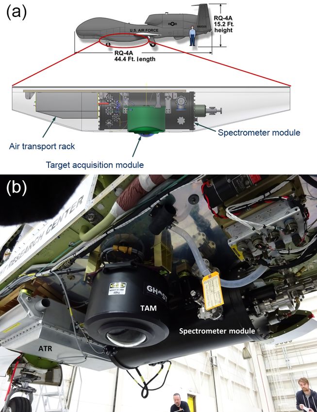
Figure 17. CAST-ATTREX Global Hawk flight paths in February and March 2015: 26 February 2015 in yellow (range flight), 5 March in
green (science flight), and 10 March in red (science flight).
Table 7. Summary of Global Hawk flights which took place under the CAST-ATTREX project during February and March 2015.
Date (UTC) Take-off time, UTC (local) Duration Description
26 February 2015 15:00 (07:00) 6.6 h Range flight over desert and mountainous regions close to Edwards,
CA.
5 March 2015 04:00 (20:00) 21 h Science flight over tropical eastern Pacific targeting profiles through the
tropical tropopause layer. About 10 h of cloud-free daylight conditions
on the return leg were suitable for GHOST observations.
10 March 2015 17:00 (10:00) 11.5 h Science flight over eastern Pacific targeting clear skies for GHOST ob-
servations. The southbound flight leg was specifically located and timed
to coincide with an OCO-2 overpass, whilst GOSAT also passed over
the measurement region around the same time.
vapour, ice crystals, and ozone, as well as an air sampling to coincide both spatially and temporally with an overpass
system for post-flight laboratory analysis of chemical com- of the NASA OCO-2 (Orbiting Carbon Observatory, Crisp
position. et al., 2017; Eldering et al., 2017) satellite during cloud-free
The CAST project (Harris et al., 2017) had similar objec- conditions as shown in Fig. 18, providing an opportunity for
tives, looking at atmospheric composition and structure in comparison of the two data sets. In Sect. 5 we focus on this
the tropics. The 2015 Global Hawk flights, operated jointly segment of the 10 March flight when presenting the first set
with ATTREX, met the project objectives to demonstrate of results from the GHOST spectrometer. This part of the
two new technologies for airborne atmospheric measure- flight also coincided with a GOSAT (Greenhouse Gases Ob-
ments: GHOST and an ice crystal imaging probe called AI- serving SATellite, Kuze et al., 2009) overpass of the region,
ITS (the Aerosol Ice Interface Transition Spectrometer, Stop- with the sounding locations shown in yellow in Fig. 18.
ford et al., 2015). The two CAST instruments therefore had
opposing requirements for atmospheric conditions during
flight, as GHOST requires the sky to be as cloud-free as pos- 5 First GHOST results from the CAST-ATTREX
sible for optimal results, whereas the AIITS team would ben- Global Hawk flights
efit from flying through cloud as much as possible to fully
This section describes the first in-flight results obtained from
test their instrument. The two science flights listed in Table 7
the GHOST spectrometer, taken during the CAST-ATTREX
each address one of these two requirements, with a large pro-
10 March 2015 Global Hawk flight. The first part of this sec-
portion of the 5 March 2015 flight dedicated to vertical pro-
tion outlines the optimal estimation method used to estimate
filing through the TTL.
GHG concentrations from the measured spectra, including
The flight on 10 March 2015, on the other hand, was tai-
steps taken to allow for a systematic channelling effect ob-
lored towards the requirements of GHOST (cloud-free skies
served in the data, whilst the second part presents the results
during daylight hours). One of the flight legs was designed
themselves and assesses their quality.
Atmos. Meas. Tech., 11, 5199–5222, 2018 www.atmos-meas-tech.net/11/5199/2018/N. Humpage et al.: An airborne shortwave-infrared spectrometer for remote sensing of greenhouse gases 5213
Figure 18. (a) 10 March Global Hawk flight path (red) plotted with sample locations of OCO-2 (green) and GOSAT (yellow) soundings. The
blue–white colour scale shows the cloud fraction retrieved from MODIS (Moderate Resolution Imaging Spectroradiometer) observations. (b,
c) Images from the GHOST visible camera taken during the OCO-2 overpass. Panel (b) shows cloud-free conditions towards the beginning
of the flight leg, whilst (c) shows sparse cloud cover encountered towards the end of the flight leg.
5.1 Retrieval of GHG total column observations from The forward model of the retrieval algorithm employs the
GHOST spectra LIDORT radiative transfer model (Spurr, 2008), which we
use to calculate the upwelling spectral radiance at the height
The calibrated GHOST spectra (an example of a radiance of the aircraft. The monochromatic spectrum is then passed
spectrum recorded during this flight is shown in Fig. 19) through the instrument model where it is convolved with the
have been analysed using the University of Leicester full instrument line shape function to simulate the measured ra-
physics retrieval algorithm. This algorithm uses an itera- diances at the appropriate spectral resolution. The inverse
tive retrieval scheme based on Bayesian optimal estima- method employs the Levenberg–Marquardt modification of
tion (Rodgers, 2000) to estimate a set of atmospheric, sur- the Gauss–Newton method to find the estimate of the state
face, and instrument parameters, referred to as the state vec- vector with the maximum a posteriori probability, given the
tor, from the radiance spectra measured by GHOST via calls measurement (Connor et al., 2008).
to a forward model and an inverse method. The forward Here, we only present results from a fit to the CO2 and
model describes the physics of the measurement process CH4 spectral bands in Band 2A (coloured green and blue
and relates measured radiances to the state vector. It con- respectively in Fig. 19) to infer the ratio of CO2 to CH4 , ac-
sists of a radiative transfer (RT) model coupled to a model cording to the proxy retrieval approach (Parker et al., 2011;
of the solar spectrum to calculate the monochromatic spec- Frankenberg et al., 2006). The advantage of this approach is
trum of light that originates from the sun, passes through the reduced sensitivity to aerosols due to a cancellation of
the atmosphere, reflects from the Earth’s surface or scatters the aerosol effects in the retrieved CO2 and CH4 columns, so
from molecules or particles in the atmosphere, and is mea- subsequently aerosols do not have to be considered for the
sured by the instrument (Boesch et al., 2006, 2011). We use retrieval. In using the proxy method, we assume that very
output from two re-analysis models as the a priori estimate similar distributions of light paths contribute to the observed
of the atmospheric state: the Copernicus Atmosphere Mon- spectra at the absorption wavelengths of both the gas of in-
itoring Service (CAMS, Bergamaschi et al., 2007, 2009) terest and its proxy for the total air column, introducing the
for CH4 profiles as a function of pressure, and Carbon- requirement that we use spectrally neighbouring fitting win-
Tracker (CT2016, Peters et al., 2007, with updates docu- dows. In addition, the method assumes that our measurement
mented at http://carbontracker.noaa.gov, last access: 29 Au- exhibits equivalent sensitivity to both gases at the heights at
gust 2018) for similar profiles of CO2 , H2 O, and temperature.
www.atmos-meas-tech.net/11/5199/2018/ Atmos. Meas. Tech., 11, 5199–5222, 2018You can also read