Megafauna community assessment of polymetallic-nodule fields with cameras: platform and methodology comparison
←
→
Page content transcription
If your browser does not render page correctly, please read the page content below
Biogeosciences, 17, 3115–3133, 2020
https://doi.org/10.5194/bg-17-3115-2020
© Author(s) 2020. This work is distributed under
the Creative Commons Attribution 4.0 License.

Megafauna community assessment of polymetallic-nodule fields
with cameras: platform and methodology comparison
Timm Schoening1, , Autun Purser2, , Daniel Langenkämper3 , Inken Suck1 , James Taylor4 , Daphne Cuvelier5,6 ,
Lidia Lins7 , Erik Simon-Lledó8 , Yann Marcon9,10 , Daniel O. B. Jones8 , Tim Nattkemper3 , Kevin Köser1 ,
Martin Zurowietz3 , Jens Greinert1 , and Jose Gomes-Pereira11,6
1 GEOMAR      Helmholtz Centre for Ocean Research, Kiel, Germany
2 Alfred Wegener Institute, Helmholtz Centre for Polar and Marine Research, Bremerhaven, Germany
3 Biodata Mining Group, Bielefeld University, Bielefeld, Germany
4 Senckenberg am Meer, Wilhelmshaven, Germany
5 MARE – Marine and Environmental Sciences Centre, IMAR – Instituto do Mar, Horta, Portugal
6 Centro OKEANOS, Universidade dos Açores, Horta, Portugal
7 Department of Biology, Ghent University, Ghent, Belgium
8 National Oceanography Centre, Southampton, UK
9 University of Bremen, MARUM Center for Marine Environmental Sciences, Bremen, Germany
10 Department of Geosciences, University of Bremen, Bremen, Germany
11 Naturalist, Lda., Atlantic Naturalist Association, Horta, Portugal
 These authors contributed equally to this work.

Correspondence: Timm Schoening (tschoening@geomar.de)

Received: 6 September 2019 – Discussion started: 14 October 2019
Revised: 23 April 2020 – Accepted: 30 April 2020 – Published: 19 June 2020

Abstract. With the mining of polymetallic nodules from the          show that, for many categories of megafauna, differences in
deep-sea seafloor once more evoking commercial interest,            image resolution greatly influenced the estimations of fauna
decisions must be taken on how to most efficiently regulate         abundance determined by the annotators. This is an impor-
and monitor physical and community disturbance in these             tant finding for the development of future monitoring leg-
remote ecosystems. Image-based approaches allow non-                islation for these areas. When and if commercial exploita-
destructive assessment of the abundance of larger fauna to be       tion of these marine resources commences, robust and veri-
derived from survey data, with repeat surveys of areas possi-       fiable standards which incorporate developing technological
ble to allow time series data collection. At the time of writing,   advances in camera-based monitoring surveys should be key
key underwater imaging platforms commonly used to map               to developing appropriate management regulations for these
seafloor fauna abundances are autonomous underwater vehi-           regions.
cles (AUVs), remotely operated vehicles (ROVs) and towed
camera “ocean floor observation systems” (OFOSs). These
systems are highly customisable, with cameras, illumination
sources and deployment protocols changing rapidly, even             1   Introduction
during a survey cruise. In this study, eight image datasets
                                                                    The increasing demand for tech metals for consumer and
were collected from a discrete area of polymetallic-nodule-
                                                                    industrial high-technology devices has again stoked interest
rich seafloor by an AUV and several OFOSs deployed at var-
                                                                    in the potential use of global deep-sea polymetallic-nodule
ious altitudes above the seafloor. A fauna identification cata-
                                                                    fields as exploitable sources of these materials in the near
logue was used by five annotators to estimate the abundances
                                                                    future (Yamazaki and Brockett, 2017; Peukert et al., 2018a;
of 20 fauna categories from the different datasets. Results
                                                                    Volkmann and Lehnen, 2018). This increasing interest, si-

Published by Copernicus Publications on behalf of the European Geosciences Union.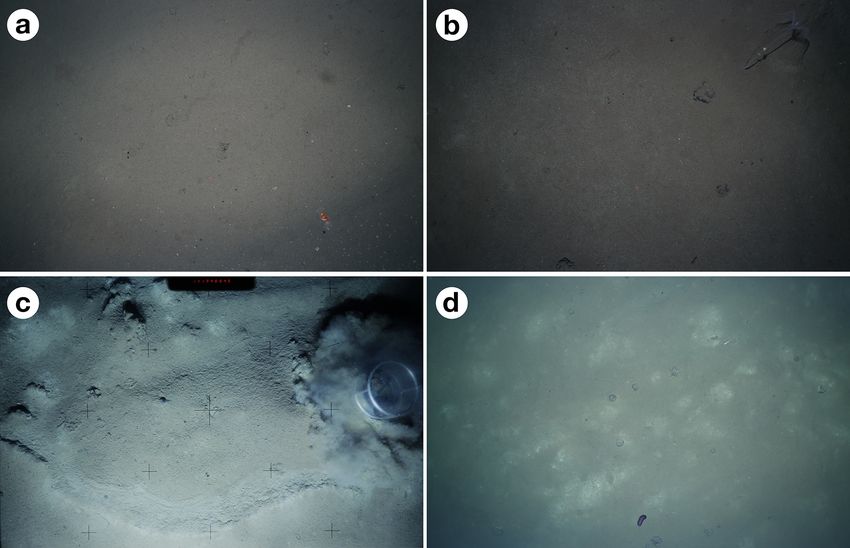
3116                   T. Schoening et al.: Megafauna community assessment of polymetallic-nodule fields with cameras

multaneously driving the technological development of ma-         impact study. However, nearby reference areas not impacted
rine mining equipment and the granting of exploration con-        by the experiment indicated pronounced temporal variability
tracts within the Clarion–Clipperton Fracture Zone (CCFZ)         in megafauna communities in the region (Bluhm, 2001). The
(Lodge et al., 2014), has stimulated several recent European      ploughing activities also created a sediment plume that reset-
research projects (e.g. JPI Oceans MiningImpact 1–2 and           tled in the surrounding areas. In these indirectly impacted ar-
MIDAS). These projects focused on the study of these re-          eas, animal densities declined immediately after the plough-
mote ecosystems to better understand the nodule distribu-         ing event, and although densities later (i.e. after 3 and more
tion (Peukert et al., 2018b) as well as the community struc-      years) appeared to be greater than in the pre-impact study
ture of macrofauna (De Smet et al., 2017) and megafauna           reference areas (Bluhm, 2001), megafaunal community com-
(Simon-Lledó et al., 2019b), ecosystem functioning, and sus-      position in these areas remains significantly different than
ceptibility to damage following anthropogenic perturbation        that found within plough tracks and reference areas (Simon-
and/or resource removal (Vanreusel et al., 2016; Jones et al.,    Lledó et al., 2019a). As has been reported from many ecosys-
2017). Despite the occurrence of nodule fields in the Atlantic,   tems, the methodologies used to quantify fauna abundances
Pacific and Indian oceans, the majority of research efforts       and species diversity can greatly influence assessments. This
have been focused on the CCFZ, located in the northern–           challenges the direct comparison of regions sampled differ-
central Pacific, as it has the highest known density of nod-      ently (Lam et al., 2006; Wilson et al., 2007; Murphy and
ules (Mullineaux, 1987; Jones et al., 2017; Simon-Lledó           Jenkins, 2010; Jaffe, 2014). Further, small variations in de-
et al., 2019b), and the Peru Basin (southern–central Pa-          ployment techniques or sampling set-ups (e.g. variables such
cific) (Bluhm, 2001; Purser et al., 2016; Simon-Lledó et al.,     as mesh size or trawl speed for direct sampling, illumination,
2019a). Both regions have been considered to potentially          camera and lenses for remote sampling) can also influence
host commercial abundances of nodules at some point in            the quality of the collected data (Purser, 2015), hampering
history. Focused scientific study commenced in the 1980s,         comparison within the same study site. In this study, a range
with simulated mining studies conducted in both areas, to as-     of commonly used imaging platforms were deployed at vary-
sess the response of fauna to mining activities (Lam et al.,      ing altitudes above the seafloor to survey megafauna across
2006). These studies are summarised in Jones et al. (2017),       a defined region of the DEA, which is a region of the Peru
with the “DISturbance and COLonization” (DISCOL) long-            Basin with abundant seafloor nodule coverage. These col-
term study in the Peru Basin being the most extensively           lected images were then placed into the online image anno-
perturbated region of seafloor studied to date (Thiel, 2001).     tation system BIIGLE (Langenkämper et al., 2017), and the
Prior to the 1980s, only occasional opportunistic fauna col-      fauna was identified in the different image sets by five anno-
lection records had been published from these areas. Since        tators using a predetermined taxon catalogue. The hypothesis
the 1980s, regular biological box core sampling has been          tested was that both composition and abundance observations
conducted in the CCFZ, whereas the majority of fauna sam-         of fauna differ between different imaging methodologies in
pling in the DISCOL area has been image based, augment-           polymetallic-nodule fields. This study aims to provide useful
ing some initial trawl sampling deployments. The DISCOL           information and guidance on how future optical monitoring
experiment was designed to simulate the effects that phys-        of these and other remote ecosystems should most effectively
ical disturbances, such as those caused by future commer-         and efficiently be conducted, should commercial exploitation
cial deep-sea mining, might have on the seafloor and its in-      of these remote resource fields commence.
habitants. In 1989, a plough harrow was used to create a
large-scale disturbance on the seafloor in the DISCOL ex-         1.1   Polymetallic nodules and associated fauna
perimental area (DEA). The plough harrow was deployed
78 times in 1989, with the aim of driving all polymetallic        Polymetallic nodules, as well as representing a potential
nodules from the sediment surface into the underlying soft        commercial resource (Burns and Burns, 1977; Watling,
sediments (Fig. 1) (Bluhm, 2001). This ploughing action de-       2015; Petersen et al., 2017), are a key hard substratum that,
stroyed the majority of surface megafauna and drove man-          in combination with the background soft sediment, act to
ganese nodules within 8 m diameter swathes down into the          increase habitat complexity and promote the occurrence of
sediments. As a result, fauna that lived attached to the nod-     some of the most biologically diverse seafloor assemblages
ules was removed and thus destroyed. The soft-bottom com-         in the abyss (Vanreusel et al., 2016; Simon-Lledó et al.,
munity, however, did show signs of recovery 7 years after         2019c). Nodule fields at the abyssal Pacific can be comprised
the plough disturbance. Several monitoring cruises of the im-     of nodules of up to 25 cm in diameter (Sharma, 2017) and
pacted areas commenced in the following years and decades.        at a range of abundance densities (e.g. 0–30 kg m−2 ; Mewes
The repopulation of the disturbed areas by highly motile          et al., 2014). Processes of nodule formation are uncertain,
and scavenging animals started shortly after the area was         though each individual nodule tends to form around a small
ploughed (Bluhm, 2001). Seven years later hemi-sessile ani-       shell fragment, shark tooth or equivalent small hard foci.
mals had returned to the disturbed areas, but the total abun-     With growth, individual nodules become heavier and capa-
dance of soft-bottom taxa was still low compared to the pre-      ble of supporting, as an anchor or hard substrate, a range

Biogeosciences, 17, 3115–3133, 2020                                                 https://doi.org/10.5194/bg-17-3115-2020
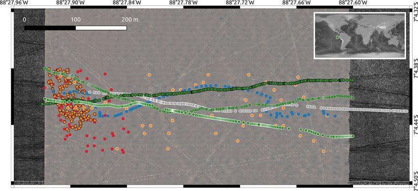
T. Schoening et al.: Megafauna community assessment of polymetallic-nodule fields with cameras                                       3117

Figure 1. Overview map of imaging locations of the eight different datasets. DSA (green dots, grey border), DSB (green dots, black border),
DSC (blue dots), DSD (green dots, white border), DSE (orange dots, black border), DSF (grey dots), DSG (orange dots, white border) and
DSH (red dots). The world map in the top right corner shows the geographical location of the DISCOL area in the eastern South Pacific
(green dot; © NOAA, Amante and Eakins, 2009). The study area covers ca. 600 m×150 m. The background map shows another photo
mosaic, created from the full image set of which DSG is a subset. Criss-crossing lines are plough tracks by the mining simulation in 1989.

of larger filter-feeding organisms (Tilot et al., 2018; Simon-          it is important to highlight also the gaps in current knowl-
Lledó et al., 2019c), such as sponges (stalked – Kersken                edge and that any management plans developed should take
et al., 2018; encrusting – Lim et al., 2017), stalked and               these shortfalls into consideration. At the time of writing it
non-stalked crinoids, soft and hard corals (Cairns, 2016),              is clear even from the sparsity of published megafauna pa-
xenophyophores (Gooday et al., 2017), sabellid worms, etc.              pers from nodule regions that these ecosystems are not all
(Bluhm, 2001). Sessile organisms in turn support a diverse              alike. The Peru Basin region of the South Pacific seems to
array of mobile and sessile epibenthic organisms, including             support a generally higher abundance of stalked fauna than
further sponges, corals and worms as well as mobile and                 the Clarion–Clipperton Fracture Zone (CCFZ) nodule do-
semi-mobile fauna such as amphipods, isopods, anemones,                 mains (Bluhm, 2001; Vanreusel et al., 2016). Some large
brooding octopodes (Beaulieu, 2001; Purser et al., 2016)                types of megafauna, such as benthic octopodes, have thus far
and many others (Vanreusel et al., 2016). Although soft-                only been observed within these nodule ecosystems in the
sediment stalked sponge fauna is found in nodule-abundant               South Pacific (Purser et al., 2016), as have some fish species
regions, the nodule-based epifauna supports increased local             (Drazen et al., 2019), despite the recent increased sampling
biodiversity and abundance of species. In addition to provid-           effort across the CCFZ. Conversely, the abundant sessile
ing a hard substrate for living attachment, nodules also in-            sponges recently characterised from the CCFZ, Plenaster
crease the range of hydrodynamic niches available to the lo-            craigi, (Lim et al., 2017), are not apparent in images or anal-
cal ecosystem fauna (Mullineaux, 1989) and add complexity               ysed samples collected from south of the Equator. Whether
to food fall transport pathways. Recent cruise observations             these discrepancies are due to oceanographic, nutrient or
from the DISCOL region showed rapid transport of dead py-               habitat niche differences is not yet known. It may be con-
rosomes, following a surface bloom, to the seafloor (Boetius,           sidered that the larger nodule sizes found in the Peru Basin
2015). These dead pyrosomes were then hydro-dynamically                 region are more suitable as anchors of sufficient stability for
trapped by benthic currents alongside nodules, providing a              stalked fauna to allow brooding by octopodes for the hypoth-
local food supply to the nodule community which might oth-              esised years required by deep-sea incirrates (Purser et al.,
erwise have been transported from the region by the ambi-               2016). Another major absence in the scientific dataset is sam-
ent benthic flow conditions. This flow dynamic variability              pled voucher specimens from nodule provinces. Opportunis-
also impacts the habitat niches available for infauna (across           tic direct sampling by remotely operated vehicles (ROVs) has
all infauna size classes) below and surrounding the nodules,            taken place on a limited scale, though the ground-truthing of
with their presence influencing local biogeochemical activity           image and video data collected by ROVs and autonomous un-
and oxygen penetration pathways. At this crucial time point             derwater vehicles (AUVs) at the species level is, at present,
in research into polymetallic nodules and associated fauna,             not possible. Though this is an obvious disadvantage over di-

https://doi.org/10.5194/bg-17-3115-2020                                                         Biogeosciences, 17, 3115–3133, 2020
3118                    T. Schoening et al.: Megafauna community assessment of polymetallic-nodule fields with cameras

rect sampling of the seafloor (e.g. by trawl) to determine the      the associated human impacts of monitoring programmes
present fauna mix, this is perhaps to some extent countered         should be as little as possible. We therefore focus within this
by the far larger areas which may be surveyed rapidly by            paper on the contrasting suitability of various image-based
towed and remote camera systems – an important point given          approaches for assessing fauna abundance in polymetallic-
the extremely sparse distribution of many fauna individuals         nodule ecosystems. Furthermore, image data can be made
of morphospecies in nodule ecosystems (Bluhm, 2001; Van-            publicly available to regulators, interested NGOs and other
reusel et al., 2016; Purser et al., 2016; Simon-Lledó et al.,       players easily via online platforms (Langenkämper et al.,
2019b). These sparse distributions make impact assessments          2017), allowing these stakeholders to conduct their own stud-
more problematic than for denser fauna categories, which            ies or analyses with the same primary data. To assure reli-
have historically been subject to the direct impact by the off-     able monitoring, contractors need to publish data including
shore fishery or petrochemical industries, such as coral and        uncorrupted location and timing metadata. The acquisition
sponge reefs, where atolls and accumulations can be directly        technology of that metadata needs to be fraud-proof (e.g. by
surveyed pre- and post-cruise, either via imaging or direct         incorporating navigation data into the imagery). In case of
sampling (Purser, 2015; Howell et al., 2016; Huvenne et al.,        monitoring activities utilising directly collected fauna from
2016). Whether future management plans favour a direct or           box core, multicore or ROV collection, much of the mate-
an image-based monitoring approach to megafauna diversity           rial will be processed once, by one lab, and can degrade dur-
and stock assessment, the requirement to fill these holes in        ing the processing steps, preventing further studies. Image
extant voucher specimen collections from these regions is           data also facilitate the straightforward archiving of collected
equally prescient.                                                  data (Schoening et al., 2018) for later comparison with subse-
                                                                    quent images, potentially collected up to decades after exper-
1.2    Potential impacts associated with nodule extraction          imental or industrial disturbance, to assess long-term recov-
                                                                    ery rates. Given the extremely long lifespans of many deep-
Nodule collection will locally remove the major source of           sea organisms (Roark et al., 2009; Norse et al., 2012), this
hard substrates in nodule field areas, rendering the remain-        is an important consideration when developing monitoring
ing habitat unsuitable for some fauna (i.e. suspension feed-        strategies for efficient and useful impact assessment within
ers), as observed in experimental mining studies in the CCFZ        these ecosystems.
(Vanreusel et al., 2016; Jones et al., 2017) and DISCOL ar-
eas (Simon-Lledó et al., 2019a). Further, depending on the          1.4     Factors determining the quality of deep-sea image
removal technique, the seafloor will likely be perturbed, with              data
compaction tracks potentially formed and all overcast by
plume deposits (Jones et al., 2017; Sharma, 2019). These fea-       Samples collected by box cores, multicores or trawl are di-
tures will increase the complexity of biogeochemical activity       rectly related to the surface area sampled. In this case, the
in the region (Paul et al., 2018) and influence local hydro-        type of trawl or corer may influence the comparability of the
dynamic conditions. Experimental tracks made with both an           results to some extent (i.e. net size and tow speed important
epibenthic sled (Greinert, 2015) and plough harrow (Bluhm,          for trawls, closing mechanism for box corers). For image-
2001) have created seafloor micro-topography which focused          base derived data, there are possibly a greater number of fac-
the deposition of salps following a surface bloom event             tors affecting the estimations of fauna abundance. The most
which occurred during SO242-2 (Boetius, 2015). Such lo-             significant of those are introduced below.
calised food input variability in the deep sea will likely result
in a further modification of the fauna communities found in         1.4.1    Camera optics
these exploited regions.
                                                                    The area of seafloor which may be imaged by an optical plat-
1.3    Methodologies for fauna abundance assessment                 form is determined by the lens parameters used in the camera
                                                                    system, distance and orientation to the seafloor, sensitivity of
Box coring and multicoring are common survey methods in             the system to motion and illumination, and a range of other
impact assessments and monitoring programmes, conducted             factors (Jaffe, 2014). Larger areas of the seafloor can be im-
to assess impacts on small fauna (e.g. less than 1 cm) follow-      aged with wide-angle or “fisheye” camera systems (Kwas-
ing an anthropogenic impact event (Gage and Bett, 2005).            nitschka et al., 2016), though there is an associated vignetting
For larger fauna, image-based surveys usually provide much          effect rendering the details collected from the extremities of
more accurate estimations of benthic taxa richness and nu-          an image less rich than areas of seafloor more directly located
merical density than traditional trawling techniques (Morris        below the lens centre (Purser et al., 2009; Cauwerts et al.,
et al., 2014; Ayma et al., 2016) and have no direct physi-          2012). The raw images collected by those camera systems
cal impact on the ecosystem being investigated. When plan-          can appear quite distorted, and manual labelling of fauna
ning to assess polymetallic-nodule fauna abundance follow-          within these images is more difficult towards the edges of
ing commercial exploitation of these remote resource fields,        each image. Digital post-processing of these distorted images

Biogeosciences, 17, 3115–3133, 2020                                                    https://doi.org/10.5194/bg-17-3115-2020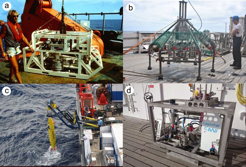
T. Schoening et al.: Megafauna community assessment of polymetallic-nodule fields with cameras                              3119

can be reasonably straightforward when the arrangement of         1.4.3   Platform altitude
optics for an imaging platform is known, and for larger fauna
these processed images can be suitable for subsequent analy-      The distance to an object can greatly alter the quality of an
sis (Schoening et al., 2016a, 2017). However, image process-      image. Although this may sound like a straightforward pa-
ing cannot create “newly improved” data, and therefore there      rameter, it may play a hugely important role when analysing
will always be a loss of information at the image extremities     fauna abundances in an area. Maintaining a uniform altitude
after lens correction. Image analysis could therefore focus on    throughout and between survey deployments is highly desir-
central parts of the image, and the boundary area of images       able (i.e. to standardise the object and/or fauna detectability
could be used to display, for example, navigation metadata.       rates) but may be difficult. In regions of the World Ocean
Lenses of a more “telephoto” or narrower angle will allow         where the seafloor is highly complex, such as at deepwa-
collection of less distorted images, though these collected       ter coral reefs (Purser et al., 2009) or within canyon sys-
images will capture a significantly smaller area of seafloor      tems (Orejas et al., 2009), it can be a struggle to main-
than may be achieved with wider-angle systems.                    tain an equal distance from camera optics from towed, au-
                                                                  tonomous, remote and submersible-based imaging platforms
1.4.2   Illumination and power provision                          to the seafloor. For polymetallic-nodule fields, however, the
                                                                  seafloor is generally fairly uniform in depth, with very gen-
The deep sea is a dark environment with no sunlight penetra-      tle slopes more the norm than occasional sudden slopes or
tion. It is therefore essential that camera systems are supple-   cliff walls. Even so, towed platform altitude stability can be
mented by artificial illumination. To provide sufficient illu-    greatly influenced by operator skill, experience, environmen-
mination for video and still-camera systems, abundant power       tal conditions (i.e. wave conditions at surface) or ship infras-
reserves must either be mounted on the platform or deliv-         tructure (winch operational parameters and presence or ab-
ered via a cable from the support vessel. The amount of           sence of heave compensators). AUV imaging platforms are
power which can be provided to a platform is determined by a      improving in stability and mission planning at a rapid rate
range of design and operational parameters. AUVs for exam-        (McPhail et al., 2010; Yu et al., 2018), and maintaining flight
ple must remain reasonably lightweight and must carry suffi-      altitudes is now a standard surveying procedure. Operations
cient power to provide mobility and to take images at depth.      with these expensive devices tend to err on the side of cau-
Towed camera systems, in contrast, are always attached to         tion; ground tracking is often set with a conservative 5–10 m
a cable (e.g. coaxial, fibre-optic) which may provide suffi-      flight altitude. At these higher flight altitudes, more light is
cient power for continuous seafloor illumination. Positioning     required to illuminate the seafloor than when a comparable
of the lights on an imaging platform can be difficult, and op-    AUV is deployed close to the seafloor (see Sect. 2.1.6).
timising the spread of light, i.e. maintaining an equal light
balance across the imaged area, can be challenging. Illumi-       1.4.4   Data volume
nation vignetting can be partially addressed prior to analysis
by excluding the image edges from analysis (Purser et al.,        Pioneer image-based studies in polymetallic-nodule fields
2009; Marcon and Purser, 2017). Given that AUVs must              were conducted with analogue film-based camera systems
carry all required power (for mobility and imaging) with          (although live, black and white seafloor views were provided
them, this can result in a less-than-optimal illumination of      to towed systems via a basic TV camera set-up) (Bluhm,
the seafloor (see Sect. 1.4.3). There is no doubt that light-     2001). This limitation constrained deployments to the col-
emitting diode (LED) technology will become more efficient,       lection of a few 100 s of images. At present, camera systems
but at present these prevalent lower-light-condition datasets     can deliver many images per second, even under low-light
constrain the seafloor resolution which may be achieved dur-      conditions. This potentially high flow of image data, how-
ing imaging surveys. Additionally, when the lights and cam-       ever, requires either an adequate digital storage space on the
era are mounted close to each other, a significant amount of      imaging platform (Kwasnitschka et al., 2016) or the facil-
light might be scattered by the water column into the cam-        ity to be transferred directly to a shipboard storage system
era, leading to a degraded “foggy” image, which is an is-         (Purser et al., 2018). This increased data flux allows for more
sue for small platforms and/or high-altitude photography. Fi-     complete spatial studies of the seafloor to be made with an
nally, the colour spectrum of the light also needs to be con-     imaging platform, but to get this additional information from
sidered, as for instance the returned yellow, orange and red      the dataset, increased processing time is required.
components of the signal may be too weak to support taxo-
nomic identification, depending on the type of light source.      1.4.5   Dataset resolution
The illumination system needs to be set up to accommodate
the target altitude of the camera platform above the seafloor     Image resolution is derived from a combination of the cam-
as well as the expected altitude variation.                       era optics and the deployment altitude and allows comparing
                                                                  image datasets numerically. The camera optics determine the
                                                                  pixel resolution (usually in the tens of megapixels for state-

https://doi.org/10.5194/bg-17-3115-2020                                                  Biogeosciences, 17, 3115–3133, 2020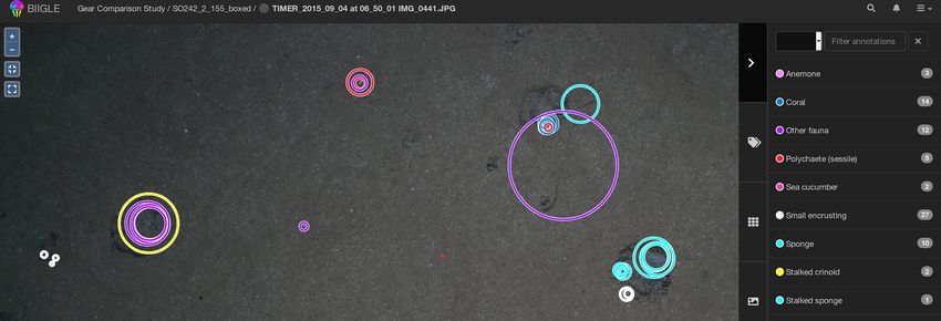
3120                   T. Schoening et al.: Megafauna community assessment of polymetallic-nodule fields with cameras

of-the-art camera systems). The field of view of the camera       SO242-2 (DSE –DSH ) in 2015. DSH was created by produc-
objective lens and the deployment altitude determine the im-      ing a mosaic of the seafloor from overlapping AUV imagery
age footprint, i.e. the area in square metres that is covered     and then dividing the mosaic into smaller image tiles for
by a single image acquisition. These two values can be com-       fauna analysis. All image sets were analysed by five anno-
bined to a measure of megapixels per square metre (MP m−2 )       tators, a1 –a5 , using a predesigned fauna catalogue to label a
or the numerically identical pixels per square millimetre to      selected group of 20 fauna categories ωa –ωt within each dis-
analyse the annotator performance and fauna density esti-         crete image (see Fig. 2). The term category refers to an arbi-
mates consistently.                                               trary object type, extending across various taxonomic levels
                                                                  and also including the category litter. The group of annota-
1.4.6   Time series studies                                       tors selected the 20 categories by including fauna that is fre-
                                                                  quent enough for statistical interpretation. The 20 categories
To determine the level of impact an event has had on a spe-       neither cover all objects visible in the images nor represent
cific region of seafloor, repeated visits to a locale are re-     all the fauna known to occur in the area. The majority of cat-
quired. It is important to conduct baseline and impact mon-       egories represented morphotypes and could thus potentially
itoring surveys in a region-specific manner to accommodate        include different cryptic species. Numbers of annotations per
differences in faunal composition. Baseline information ac-       category and per dataset vary. No organism size cut-off was
quired in one nodule area (e.g. the CCFZ) cannot directly be      defined for annotation; instead the image resolution deter-
transferred to another (e.g. the Peru Basin). Ideally, a num-     mines which size of objects are still discernible. From this
ber of surveys at differing times of the year would be con-       labelling effort, the densities of the various identified fauna
ducted before an impacting event to gauge the background          categories in each dataset were statistically compared.
fauna community of a region and to identify natural variation
and seasonality in community patterns. These baseline stud-       2.1     Imaging platforms, resolutions and deployment
ies would be followed by repeated surveys at different time               altitudes
points during and after the impacting event. These repeated
visits should allow quantification of the duration and recov-     2.1.1    DSA (4.49 MP m−2 ) and DSB (3.89 MP m−2 ):
ery of impacts. Planning such a study may sound straight-                  low-altitude imagery from AWI OFOS camera
forward, but given the remoteness of many deep-sea regions,                sled
getting the same equipment and survey crew together may
be difficult. One such study, aimed at gauging the impact of      Towed still-image and video sleds are equipment often used
oil and gas exploration drilling on cold-water coral reefs on     for gleaning some information on seafloor physical and
the Norwegian margin, visually surveyed a number of reefs         megafauna community structure (examples can be found in
on five occasions (Purser, 2015). Despite these five survey       Fig. 3a, b, d). These platforms consist of a solid frame which
cruises taking place within a 3-year period in a relatively ac-   is connected to a survey vessel by an umbilical cable, in
cessible area of the Norwegian shelf, each cruise used differ-    most cases capable of supplying power and data transfer
ent ROV systems and survey protocols. Analysis of collected       between the ship and the platform. To operate, an altitude
data was further complicated by the mounting of different         above the seafloor is set by the users as a function of seafloor
camera and illumination systems on each ROV and contrast-         topographical structure, items of interest, vessel speed and
ing flight altitudes and dive plans being used for each deploy-   weather conditions. A winch operator maintains the appro-
ment.                                                             priate flight altitude above seafloor as the survey vessel tows
                                                                  the device over the requested course. These systems can
                                                                  utilise reasonably simple cable systems to allow live TV sig-
2   Methodology                                                   nals from the seafloor to reach a towing support vessel or
                                                                  modern fibre-optic cables through which high data loads can
For this comparative study of the effectiveness of vari-          be transmitted in real time. The simplicity and relatively low
ous imaging platforms for assessing megafauna abundances          costs of these towed systems, coupled with their moderate
in polymetallic-nodule ecosystems, eight distinct image           personnel requirements, have made them an attractive choice
datasets, DSA to DSH (see Table 1), were collected. All           to use in scientific expeditions, particularly in time series
datasets were acquired in a discrete area of seafloor of ca.      studies, where the same equipment is required for each re-
600 m×150 m. These eight datasets were collected by three         visit to a location. For this current study, the Alfred Wegener
different towed camera platforms (one of which was de-            Institute – Helmholtz Centre for Polar and Marine Research
ployed at several altitudes above seafloor) and an AUV (de-       (AWI) – Ocean Floor Observation System (OFOS) was used
ployed at two different altitudes above seafloor) during three    for collection of several datasets (see Table 1). Developed
research cruises. One dataset (DSC ) was acquired during          for time series analysis of the HAUSGARTEN marine time
RV Sonne cruise SO106, and the other seven were acquired          series station, the system has seen 15 years of regular use,
during RV Sonne cruises SO242-1 (DSA , DSB , DSD ) and            and numerous megafauna fauna papers have been published

Biogeosciences, 17, 3115–3133, 2020                                                  https://doi.org/10.5194/bg-17-3115-2020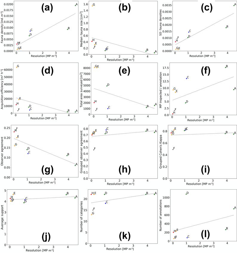
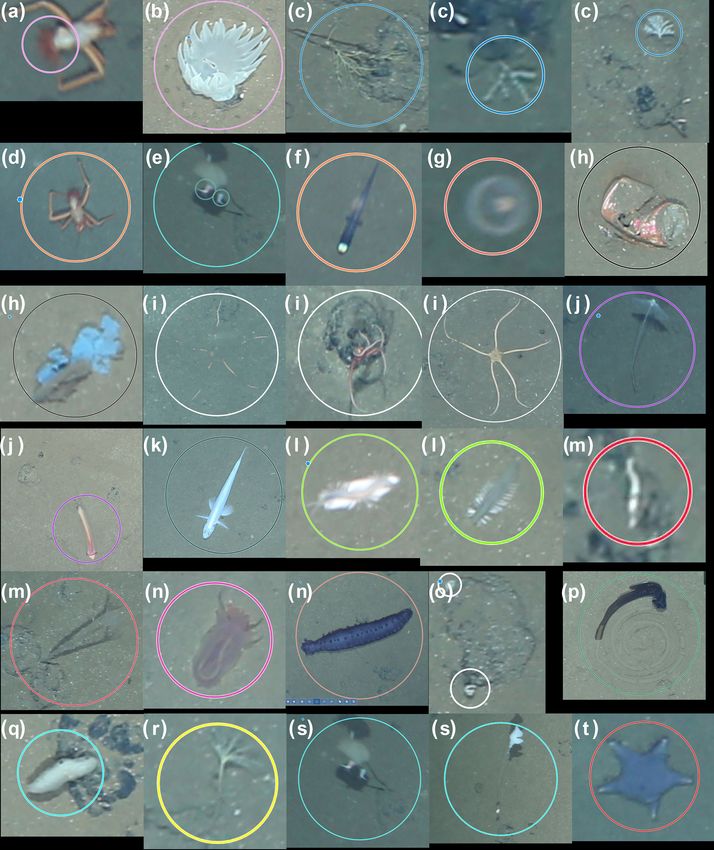
T. Schoening et al.: Megafauna community assessment of polymetallic-nodule fields with cameras                                                3121

Figure 2. Fauna categories used in the current study for the DISCOL area. Circles correspond to annotations in BIIGLE. Colours of anno-
tations visualise the category type. (a, b) Anemones, (c) corals, (d) crustacea, (e) epifauna, (f) Ipnops fish, (g) jellyfish, (h) litter, (i) Ophi-
uroidea, (j) Cladorhizidae, (l, p) Enteropneusta, (k) fish, (l) Polychaeta worms, (m) Polychaeta tubeworms, (n) Holothuroidea, (o) small
encrusting, (q) Porifera, (r) stalked crinoid, (s) stalked Porifera and (t) Asteroidea. All examples were scaled for visualisation purposes;
some, like (l) and (m), are small and close to the resolution limit.

https://doi.org/10.5194/bg-17-3115-2020                                                                Biogeosciences, 17, 3115–3133, 2020
3122 T. Schoening et al.: Megafauna community assessment of polymetallic-nodule fields with cameras
Table 1. Summary of image data collected for each dataset considered in this study. Columns marked by (∗ ) represent median values across
the dataset.
Dataset Station Date Platform Resolution∗ Altitude∗ Footprint∗ Number of
(MP m−2 ) (m) (m2 per image) images
DSA SO242-2_171 25 Sep 2015 AWI OFOS 4.49 1.6 4.9 311
DSB SO242-2_155 25 Sep 2015 AWI OFOS 3.89 1.7 5.7 206
DSC SO106_OFOS35 1997 EXPLOS OFOS 1.05 3.4 12.5 80
DSD SO242-2_233 25 Sep 2015 AWI OFOS 0.98 3.2 22.5 209
DSE SO242-1_107 17 Aug 2015 AUV Abyss 0.24 4.2 52.9 154
DSF SO242-1_111 18 Aug 2015 Custom OFOS 0.16 2.0 2.6 272
DSG SO242-1_083 13 Aug 2015 AUV Abyss 0.07 7.5 169.1 46
DSH SO242-1_102 (Mosaic) 16 Aug 2015 AUV Abyss 0.04 4.5 32.8 62
based on collected data (Bergmann et al., 2011; Pham et al., 2.1.3 DSD (0.98 MP m−2 ): high-altitude imagery from
2014; Purser et al., 2016; Taylor et al., 2016, 2017). The AWI OFOS camera sled
AWI OFOS consists of a solid frame containing vertically
downward-facing still-image and video cameras (Fig. 3). Ad- With increasing distance from the seafloor, a particular opti-
ditionally, the system mounts LED lights to a supply light cal system can image a greater area for a given set of optics,
for the video camera as well as powerful flash units to allow assuming that correct focusing, for example, can be achieved.
26 MP still images to be taken from an optimal altitude of With a doubling of distance, however, effectiveness of illu-
1.5 m above the seafloor. The AWI OFOS also incorporates mination is reduced by 75 %. For towed systems this may be
three parallel lasers to allow seafloor coverage (and fauna compensated for by additional supply of power or a greater
sizes) to be quantified in the images and video data collected. number of lights. For the current study, however, the same
Figure 4a and b show typical images collected from the DIS- AWI OFOS introduced in Sect. 2.1.1 was redeployed with
COL area from an operational altitude of 1.6 m (DSA ) and the same standard lighting configuration at a flight altitude of
1.7 m (DSB ). 3.3 m. Figure 4d shows a typical seafloor image taken from
this altitude.
2.1.2 DSC (1.05 MP m−2 ): high-altitude, digitised
analogue imagery from EXPLOS camera sled 2.1.4 DSE (0.24 MP m−2 ): low-altitude imagery from
AUV Abyss
Prior to the equipping of research vessels with fibre-optic ca-
bles, allowing HD video to be transmitted directly to the sup- During SO242-1, GEOMAR’s AUV Abyss (Linke and
port vessel during a dive, it was common practice to set up a Lackschewitz, 2016) was deployed for several photographic
low-quality video link to the seafloor to allow the operators mapping missions (see Fig. 3c). The vehicle’s original cam-
of a towed device to maintain an appropriate flight altitude era had been replaced by a Canon 6D DSLR camera and the
above the seafloor during a deployment. The scientific data Xenon strobe by an LED flash system (Kwasnitschka et al.,
collected were still images manually triggered from the ship 2016), placed 2 m from one another. The low-altitude vertical
but recorded onto analogue photographic film using a PHO- imagery of DSE was captured from a target altitude of 4.5 m,
TOSEA 5000 camera mounted on the “Exploration System” at a speed of 1.5 m s−1 and at a frame rate of 1 Hz. The sys-
(EXPLOS) towed device. This required the mounting of ac- tem was equipped with a Canon 8–15 mm fisheye lens (fixed
tual film canisters on the towed platforms, resulting in de- to 15 mm) centred in a dome port. Owing to weak illumina-
ployments with fewer than 400 images collected (the capac- tion in the outer image regions, only the central 90◦ (across
ity of standard, extended 35 mm magazines of the era). In track) or 74◦ (along track) of the fisheye images were used
1989, after the seafloor ploughing, such an analogue towed and trilinearly resampled to a picture that an ideal rectilinear
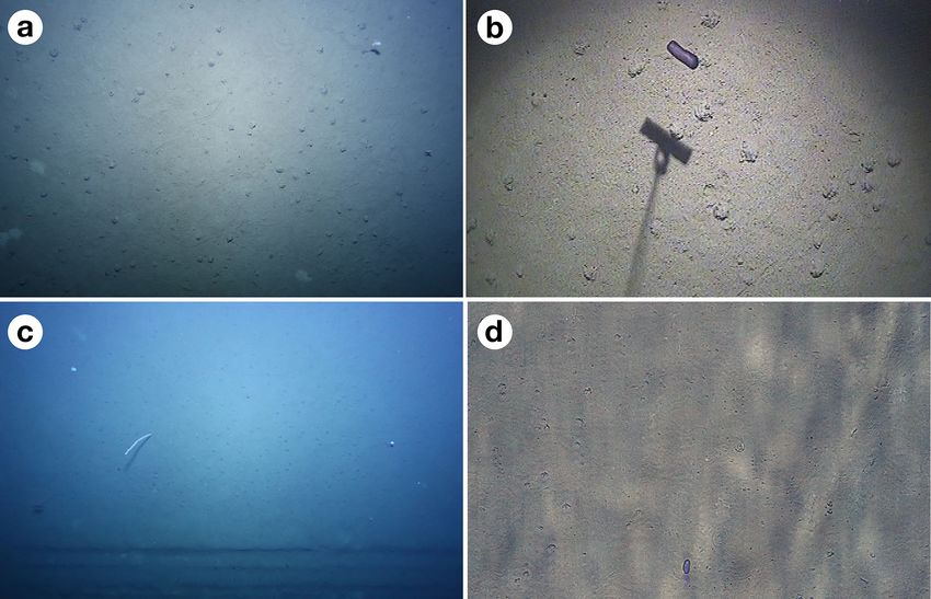
camera rig was used to image in the DISCOL area (Fig. 3a). 18 mm lens would have taken. An example picture is shown
The 1989 dataset was recently digitised by the MiningImpact in Fig. 5a.
project of the Joint Programming Initiative Ocean (JPIO) and
made available for this study. An example image is given in 2.1.5 DSF (0.16 MP m−2 ): low-altitude imagery from
Fig. 4c. custom OFOS camera sled
During SO242-1 the area of interest was surveyed with a
colour video camera (Oktopus GmbH) in conjunction with
one Oktopus HID 50 light mounted vertically on a towed
frame (see Fig. 3b). The signal was transmitted to a deck
Biogeosciences, 17, 3115–3133, 2020 https://doi.org/10.5194/bg-17-3115-2020T. Schoening et al.: Megafauna community assessment of polymetallic-nodule fields with cameras 3123 Figure 3. Imaging platforms used in the current study. (a) The EXPLOS OFOS analogue camera sled from 1997 (Schriever and Thiel, 1992). (b) A custom OFOS used during SO241-1. (c) GEOMAR AUV Abyss. (d) AWI OFOS. Figure 4. Example images of datasets DSA –DSD , with platform information and mean image footprints as follows. (a) DSA – OFOS – 4.9 m2 . (b) DSB – OFOS – 5.7 m2 . (c) DSC – OFOS – 12.5 m2 . (d) DSD – OFOS – 22.5 m2 . https://doi.org/10.5194/bg-17-3115-2020 Biogeosciences, 17, 3115–3133, 2020
3124                    T. Schoening et al.: Megafauna community assessment of polymetallic-nodule fields with cameras

Figure 5. Example images of datasets DSE –DSH , with platform information and mean image footprints as follows. (a) DSE – AUV –
52.9 m2 . (b) DSF – OFOS – 2.6 m2 . (c) DSG – AUV – 169.1 m2 . (d) DSH – AUV – 32.8 m2 .

unit (Oktopus GmbH VDT 3) and recorded using an exter-              2.1.7    DSH (0.04 MP m−2 ): low-altitude imagery from
nal video converter (Hauppauge – HD PVR), which con-                         AUV Abyss and extracted from a photo mosaic
verted the signal to .mp4 files, and was then recorded on
a PC using ArcSoft TotalMedia Extreme software. For this            AUV images of station SO242-1_102 were collected at
study, frames were extracted from these video files at a rate       ca. 4.5 m above the seabed, with 80 % along-track and 50 %
of 0.1 Hz. The custom OFOS was put together in an “ad hoc”          across-track overlap in order to build one large photo mo-
fashion, from a range of off-the-shelf components, to mimic         saic out of the images. In order to mitigate water and illu-
“pioneer” image-based methodology rather than a fully de-           mination effects otherwise dominant in the final mosaic, a
signed and integrated device. An example image is given in          robust statistical estimate of the illumination component was
Fig. 5b. Further details of the custom OFOS and its deploy-         performed. For this, each image was robustly averaged with
ments can be found in Greinert (2015).                              the seven images taken before and after, producing an image
                                                                    without nodules that represents the illumination effects. The
2.1.6   DSG (0.07 MP m−2 ): high-altitude imagery from              raw image was then – pixel-wise – divided by the illumina-
        AUV Abyss                                                   tion image and multiplied by the expected seafloor colour,
                                                                    which was obtained from box core photographs of the same
As a result of the fixed distance of roughly 2 m between the        cruise. For each track of a multi-track AUV mission, the im-
camera and light source on AUV Abyss, images taken by the           ages were registered against each other, leading to relative
above system at higher altitudes increasingly suffered from         AUV localisation information with sub-centimetre accuracy.
very strong backscatter in addition to the loss of colour re-       Afterwards, the photos were projected to the seafloor and
sulting from the large distance from the light source to the        rendered into a virtual orthophoto with a resolution of 5 mm
seafloor and back into the camera. Although the AUV imaged          per pixel (reflecting the best resolution in the fisheye images)
at altitudes above 10 m, those images were deemed of a qual-        of roughly 7 ha size. The photo mosaic was then subdivided
ity unsuited for fauna analysis. Consequently, besides the          into ca. 11 000 tiles and uploaded to BIIGLE for megafaunal
4.2 m “low-altitude” AUV imagery in DSG , AUV imagery               assessment. An example tile is shown in Fig. 5d. A simi-
acquired at 7.5 m altitude represents the dataset of maximum        lar mosaic of the same area was used in Simon-Lledó et al.
altitude in this contribution. Apart from the different altitude,   (2019a).
all capture parameters in DSG remained the same as in DSE .
An example image for this dataset is shown in Fig. 5c.              2.2     Image annotation methodology

                                                                    Within the study, 1340 seafloor images (or mosaic tiles) were
                                                                    analysed for megafauna abundance and community structure

Biogeosciences, 17, 3115–3133, 2020                                                    https://doi.org/10.5194/bg-17-3115-2020
T. Schoening et al.: Megafauna community assessment of polymetallic-nodule fields with cameras 3125
estimation (see Table 1). All images used in the study were except Fig. 7g further visualise the results of the grouped
imported into the BIIGLE online annotation system (Lan- annotations. Most obvious is the increase in fauna density
genkämper et al., 2017). Once imported, five annotators in- with imaging resolution (see Fig. 7a). This trend is mir-
spected the images independently and annotated objects by rored in the observation that the median size of the anno-
placing a circle around each instance using the BIIGLE an- tated fauna decreases with increasing resolution (see Fig. 7b).
notation interface (see Fig. 6). To assist in this, an identifica- Together it can be reasoned that the increased resolution al-
tion guide with 20 categories was produced (see Fig. 2), from lows annotating smaller objects, increasing the total amount
which the annotators could work. of individuals annotated. Nevertheless, it is also obvious
that the increased resolution comes with an increase in ob-
2.3 Observer agreement server disagreement. Figure 7c shows that the standard de-
viation of fauna densities created by the five experts in-
Manual annotation was conducted independently. To com- creases with increasing resolution. Figure 7d–f highlights
pare results from the five annotators, a1 to a5 , inter-observer the trade-off between resolution and seafloor inspection ef-
agreement was computed (Schoening et al., 2012). First, the fort. In Fig. 7d it can be seen that the increase in resolution
individual annotations of each pair of annotators were com- comes with a decrease in acquisition efficiency in terms of
pared regarding the annotation location (i.e. the detection the area per hour (m2 h−1 ) that can be imaged. This nega-
step) and annotation label (i.e. the classification step). An- tive correlation exists also when removing dataset DSG . Fig-
notations of individual experts were then grouped to gold- ure 7f shows that, although higher densities of fauna are
standard annotations to increase the robustness of the dataset detected for high-resolution datasets, it still requires man-
comparison. A gold standard is the best-possible ground truth ually inspecting more megapixels per annotation compared
information if no actual ground truth is available (Schoen- to lower-resolution datasets. The annotation effort for such
ing et al., 2016b). Grouping of annotations was conducted by high-resolution datasets is thus overproportionately large.
fusing annotations which overlap within one image and are Removing single points that appear as outliers in the differ-
of a similar size to one grouped annotation. The position and ent data dimensions (Fig. 7a–l) does not change the general
radius of a grouped annotation represent the mean of the po- trends of the correlation lines.
sitions and radii of the single, overlapping annotations. The
support of one annotation quantifies how many experts found 3.2 Observer agreement
this individual and thus ranks between 1 and 5. The label of
the grouped annotation was selected as the most frequent la- Figure 7g outlines the importance in image-based studies of
bel within the grouped annotations. Annotations that were incorporating annotations created by more than one annota-
supported by only one annotator were discarded. Also, if no tor. It shows the generally poor observer agreement in this
two annotators assigned the same label to an annotation it study when considering the single-expert annotations (see
was discarded. As a further measure of observer agreement, also Table 2). It further highlights that the observer agree-
Cohen’s kappa was computed (McHugh, 2012). ment drops with increasing image resolution, echoing the
results in Fig. 7c. When grouping the single observer an-
2.4 Fauna-specific statistical analysis notation to form the gold-standard annotations, the observer
agreement increases significantly (see Fig. 7h). This increase
The average abundance estimations of each individual fauna
is similarly reflected by Cohen’s kappa values: all but one
category computed for each of the eight image sets were de-
above 0.7, which is deemed to be “substantial agreement”
rived from the annotations made by each independent anno-
(0.6–0.8).
tator. The five density estimates obtained for each fauna cat-
egory, as generated from the labels made by the individual
3.3 Fauna-specific statistical analysis
image annotators across the eight imaging-platform datasets,
were compared using nonparametric Kruskal–Wallis tests.
The seafloor densities of the 20 categories of fauna and
These tests were conducted using the software package
seafloor features, as quantified by the five independent an-
SPSS 17.0. Significant differences were considered when
notators, are given in Fig. 8 (mobile fauna) and Fig. 9 (ses-
p < 0.05.
sile fauna). Kruskal–Wallis tests indicated that for all fauna
categories (with the exception of “molluscs”) observed, in-
3 Results dividual densities differed by imaging platform at the 95 %
threshold (“small encrusting”, “starfish”) or < 99 % thresh-
3.1 Aggregated results for datasets old (all other fauna categories). For sessile fauna, the aver-
age individual densities observed were highest across fauna
Aggregated results for various characteristics of the eight categories in DSA . Generally, the average densities for this
datasets and annotations were computed by averaging across dataset acquired at 1.6 m altitude were roughly double to
all fauna categories (see Fig. 7 and Table 2). All figures triple those observed in DSB , which was collected in the
https://doi.org/10.5194/bg-17-3115-2020 Biogeosciences, 17, 3115–3133, 20203126 T. Schoening et al.: Megafauna community assessment of polymetallic-nodule fields with cameras
Figure 6. Circular fauna identifications made by several operators using the BIIGLE software application. Each circle corresponds to one
annotation by one annotator. Colours of circles correspond to categories.
Table 2. Annotation results for the eight different datasets considered in this study.
Dataset No. annotations No. categories Observer agreement Observer agreement Cohen’s kappa Fauna density
(grouped) found (single annotators) (grouped) (grouped) (ind. m−2 )
DSA 741 22 0.06 0.65 0.75 0.0194
DSB 264 22 0.11 0.66 0.76 0.0092
DSC 78 18 0.12 0.71 0.82 0.0085
DSD 1077 22 0.14 0.66 0.81 0.0065
DSE 231 22 0.20 0.69 0.82 0.0009
DSF 70 15 0.24 0.40 0.49 0.0029
DSG 61 13 0.16 0.65 0.74 0.0007
DSH 202 22 0.23 0.66 0.77 0.0030
same year from a slightly higher median altitude of 1.7 m. seafloor based on experts’ manual annotations. Given the in-
Densities of sessile fauna derived from AUV data were gen- accuracies of about 1 % achievable with the POSIDONIA
erally lower than those derived from OFOS data. Sessile- underwater positioning system used for the majority of imag-
fauna densities derived from AUV data acquired at 4.2 m ing deployments (Peyronnet et al., 1998) and the lack of dis-
altitude (DSE ) were invariably higher than those derived tinct seafloor features in the DISCOL polymetallic-nodule
from 7.5 m AUV data (DSG ). Sessile-fauna densities deter- province, sampling exactly the same areas of seafloor was not
mined from the mosaicked images were roughly equivalent possible. Nevertheless, due to the reasonably homogenous
or a little lower than the densities determined from both nature of the seafloor (from the scale of metres to hundreds
uncombined AUV datasets (see Fig. 9). For mobile fauna, of metres) in the survey region, it seems likely that com-
trends in densities of fauna categories were less dependent parable organisms were present across areas. Temporal dif-
on the observing platform. Even though differences were in- ferences in community structure, particularly between years,
dicated as significant for many fauna categories (see Table 3), cannot be wholly discounted as explanatory factors of dif-
these differences were not clearly relatable to either imaging- ferences between datasets (Bluhm, 2001; Borowski, 2001).
platform deployment altitude or methodology and observers Highly mobile fauna, such as fish and jellyfish, can vary in
(see Fig. 8). local abundances on temporal scales of minutes, and even
the less mobile ophiuroids and holothurians can respond rel-
atively swiftly to changes in seafloor conditions, such as a
4 Discussion food fall or hydrodynamic conditions. Even so, we assume
that temporal and spatial differences between the collected
4.1 Spatial and temporal factors data are of minor significance in explaining the differences
in densities observed.
The current study attempts to estimate the effectivity of
a range of imaging devices across an overlapping area of
Biogeosciences, 17, 3115–3133, 2020 https://doi.org/10.5194/bg-17-3115-2020T. Schoening et al.: Megafauna community assessment of polymetallic-nodule fields with cameras 3127
Figure 7. Aggregated results of fauna annotations for the eight datasets (dots A–H; green: AWI OFOS; blue: EXPLOS OFOS; grey: custom
OFOS; orange: AUV Abyss; red: AUV Abyss mosaic). Dashed lines show linear regressions.
4.2 Deployment altitude and image resolution such as jellyfish and fish. Given the three dimensionality of
the habitat utilised by these organisms, observation from a
Even though it was not possible to deploy all platforms at greater altitude is beneficial, and it is thus more likely to im-
different altitudes within the same cruise, it was feasible age such fauna. This is potentially coupled with avoidance
to collect material altogether from both the AUV (two al- mechanisms triggered by the lights on the imaging platform
titudes) and the AWI OFOS (three altitudes). For virtually or the sound of thrusters (in the case of the AUV deploy-
all fauna categories used, the highest-density estimates were ments). The way in which fauna density estimations are sub-
made from data collected at the lowest deployment altitude ject to the deployment altitude does not appear to be linear or
and highest pixel resolution. At these altitudes, less water is comparable across fauna categories. Larger types of fauna,
present between the camera and the target, reducing distor- such as “stalked sponges” (see Fig. 9d) and “starfish” (see
tion and light attenuation effects. The only exceptions to this Fig. 8j), were spotted with equivalent ease across all datasets,
trend were the highly mobile, water-column-dwelling fauna, whereas smaller types of fauna, such as “sessile polychaetes”
https://doi.org/10.5194/bg-17-3115-2020 Biogeosciences, 17, 3115–3133, 20203128 T. Schoening et al.: Megafauna community assessment of polymetallic-nodule fields with cameras
Table 3. Kruskal–Wallis test assessment of whether differences in
fauna abundance derived from the DISCOL seafloor data are signif-
icant for each fauna category used in the current study. H is the test
statistic, N is the number of observers, df is degrees of freedom (i.e.
number of data types compared −1) and p is significance. P values
of less than 0.05 indicate significance at the 95 % percentile.
ω Fauna H N df p
ωa Anemone 34.09 5 7 < 0.001
ωc Coral 34.63 5 7 < 0.001
ωd Crustacea 24.20 5 7 < 0.001
ωe Epifauna 33.61 5 7 < 0.001
ωf Ipnops fish 36.92 5 7 < 0.001
ωg Jellyfish 32.86 5 7 < 0.001
ωh Litter 25.68 5 7 < 0.001
Mollusc 13.65 5 7 0.46
ωk Other fish 29.09 5 7 < 0.001
ωl Polychaete mobile 27.14 5 7 < 0.001
ωm Polychaete sessile 35.16 5 7 < 0.001
ωn Sea cucumber 23.73 5 7 < 0.001
Sea urchin 25.22 5 7 < 0.001
ωo Small encrusting 16.56 5 7 0.013
ωp Spiral worm 25.37 5 7 < 0.001
ωq Sponge 32.011 5 7 < 0.001
ωr Stalked crinoid 35.54 5 7 < 0.001
ωs Stalked sponge 23.99 5 7 < 0.001
Stalk no head 25.82 5 7 < 0.001
ωt Starfish 16.93 5 7 0.011
and “sponges” (see Fig. 9b and i), were annotated more fre-
quently in data collected from lower altitudes. These altitude- Figure 8. Mobile-fauna abundances averaged across five annotators
based trends in density estimation were observed in both that independently annotate image data collected during the eight
AUV and OFOS datasets. Interestingly, an average deploy- survey deployments.
ment altitude difference of just 10 cm, from 1.7 to 1.6 m av-
erage altitude between SO242-2 OFOS deployments, corre-
sponded to a much greater difference in fauna density es-
timations than the 1.6 m difference in deployment altitudes dressing human impacts, requires not only ecological exper-
between the 3.3 and 1.7 m datasets. Both the attenuation of tise but also support from taxonomists. Nevertheless, even
light in water and the variable impact of this reduction on the when specialists analyse the same dataset, inter-observer dif-
wavelengths of reflected light, as well as the size of the fauna ferences in annotations can be significant (Schoening et al.,
image received by the camera, likely play a role in determin- 2012; Durden et al., 2016). Here, however, differences be-
ing the fauna abundance accuracy achievable from a dataset. tween platform altitude proved to be more significant than the
This extreme subjectivity to deployment altitude of derived observer effect for all faunal categories. Therefore, given the
density estimations is an important consideration when com- sparsity of many deep-sea taxa in nodule provinces (Simon-
paring results from different deployments. Lledó et al., 2019b), the use of key species is of more ap-
plicability when determining monitoring strategies for im-
4.3 Annotator skill and observer effect pact assessment, where statistically significant differences in
abundances may reflect differences in populations of pre-
To label fauna at a species level from imagery requires a impacted or control areas and those within impacted areas.
certain amount of skill and awareness of the fauna likely These key types of fauna are likely to differ between differ-
to occur in a particular survey region. In many cases, an- ent locations and ecosystems. For deep-sea manganese nod-
notation categories will only refer to morphotypes. This is ule provinces, the level of understanding of ecosystem func-
due to the fact that most fauna in the areas is either still un- tioning is probably insufficient for selecting species and/or
known or impossible to identify from images alone. Properly taxa of major importance for the ecosystem. Certainly, some
assessing fauna occurring in a habitat, especially when ad- easily annotated types of fauna play important roles as habi-
Biogeosciences, 17, 3115–3133, 2020 https://doi.org/10.5194/bg-17-3115-2020T. Schoening et al.: Megafauna community assessment of polymetallic-nodule fields with cameras 3129
curate annotations. In either case, manual annotations need
to be quality controlled, e.g. by creating a gold standard, to
produce more reliable data. Moreover, employing several ex-
perts for the image annotation would add a considerable fi-
nancial cost to any monitoring programme. In future, it is
probable that the ongoing developments of computer algo-
rithms for resource quantification (Schoening et al., 2016a,
2017) and fauna identification (Aguzzi et al., 2009; Purser
et al., 2009; Schoening et al., 2012; Siddiqui et al., 2017;
Zurowietz et al., 2018) will allow a near-real-time assessment
of fauna abundances in a surveyed region for a given plat-
form and deployment strategy. At present, however, as com-
mercial nodule mining approaches viability, traditional mon-
itoring approaches like manual image annotation or physical
sampling are the only ones available for integration into reg-
ulatory frameworks and work plans. Nevertheless, expected
technological advances should be incorporated into the regu-
lations.
5 Conclusions
The results from the current study highlight how tightly fauna
abundance estimations in manganese nodule ecosystems may
be related to the investigative methodology used. Small dif-
ferences in imaging-platform operational altitude, illumina-
tion and lens type analysed by a particular annotator can al-
ter estimations of community structure. The results obtained
by this study are similar to other studies conducted in shal-
low reef environments (Gardner and Struthers, 2013), though
they are highly prescient given the commercial interest in
Figure 9. Sessile-fauna abundances averaged across five annotators
that independently annotate image data collected during the eight these nodule resources and the current lack in background
survey deployments. knowledge to estimate the impact of mining activities on
ecosystem function. For the first time, quantitative informa-
tion was provided on the effect of using different platform
altitudes and the resulting imagery resolution. The authors of
tat engineer species, such as the stalked fauna, which add the current study do not intend to recommend a “perfect”
the vertical axis to increase habitat niche availability (Purser imaging platform for megafauna abundance monitoring in
et al., 2016; Vanreusel et al., 2016). Biogeochemical pro- manganese nodule ecosystems, as more work is still needed
cesses within and at the sediment–seawater interface may to determine whether there are megafauna species that are
well be influenced by mega-, macro- and meiofauna not vis- of particular significance in maintaining current community
ible even in high-resolution imagery. Some large types of structures and biodiversity in the nodule regions and because
fauna spend variable amounts of time within the sediments, the commercial viability of the various platforms available
and smaller types of fauna may be below the resolution limit for study will surely change during the forthcoming years.
of the imagery. Though densities of these less-visible organ- With this study, we intend to give some general guidelines on
ism categories may be measured with a range of methodolo- how long-term monitoring studies in these regions should be
gies (Gollner et al., 2017), the number of samples required, planned to allow the collection of good-quality data which
coupled with the remoteness of resource sites, renders these can be further used in time series analyses of larger-fauna
probably inappropriate for cost effective monitoring. By pro- community composition.
viding a clear identification catalogue, ideally with a limited
number of categories (as used in the current study), annota- 1. For a given study location, a comparable survey deploy-
tors with little or no experience will be able to identify fauna ment plan should be used at each time step of analysis:
within an image set with an ample degree of confidence. For the same sensor payload, instrument platform altitude,
complex studies of detailed community change, trained sci- deployment speed, seafloor area imaged and sample unit
entific personnel would be required in order to have more ac- size.
https://doi.org/10.5194/bg-17-3115-2020 Biogeosciences, 17, 3115–3133, 2020You can also read