First investigation of perennial ice in Winter Wonderland Cave, Uinta Mountains, Utah, USA
←
→
Page content transcription
If your browser does not render page correctly, please read the page content below
The Cryosphere, 15, 863–881, 2021
https://doi.org/10.5194/tc-15-863-2021
© Author(s) 2021. This work is distributed under
the Creative Commons Attribution 4.0 License.

First investigation of perennial ice in Winter Wonderland Cave,
Uinta Mountains, Utah, USA
Jeffrey S. Munroe
Geology Department, Middlebury College, Middlebury, VT 05753, USA

Correspondence: Jeffrey S. Munroe (jmunroe@middlebury.edu)

Received: 5 June 2020 – Discussion started: 10 August 2020
Revised: 13 January 2021 – Accepted: 14 January 2021 – Published: 18 February 2021

Abstract. Winter Wonderland Cave is a solution cave at             Most elements are more abundant in the younger ice, pos-
an elevation of 3140 m above sea level in Carboniferous-           sibly reflecting reduced rates of infiltration that prolonged
age Madison Limestone on the southern slope of the Uinta           water–rock contact in the epikarst. Abundances of Al and Ni
Mountains (Utah, USA). Temperature data loggers reveal             likely reflect eolian dust incorporated in the ice. Liquid water
that the mean annual air temperature (MAAT) in the main            appeared in the cave in August 2018 and August 2019, ap-
part of the cave is −0.8 ◦ C, whereas the entrance cham-           parently for the first time in many years. This could be a sign
ber has a MAAT of −2.3 ◦ C. In contrast, the MAAT out-             of a recent change in the cave environment.
side the cave entrance was +2.8 ◦ C between August 2016
and August 2018. Temperatures in excess of 0 ◦ C were not
recorded inside the cave during that 2-year interval. About
half of the accessible cave, which has a mapped length of
245 m, is floored by perennial ice. Field and laboratory in-       1   Introduction
vestigations were conducted to determine the age and origin
of this ice and its possible paleoclimate significance. Ground-    Caves containing perennial ice, hereafter known as “ice
penetrating-radar (GPR) surveys with a 400 MHz antenna re-         caves”, have been reported from around the world (Perşoiu
veal that the ice has a maximum thickness of ∼ 3 m. Sam-           and Lauritzen, 2017). Local permafrost conditions are main-
ples of rodent droppings obtained from an intermediate depth       tained in these caves due to a combination of cold-air
within the ice yielded radiocarbon ages from 40 ± 30 to            trapping and dynamic ventilation (Luetscher and Jeannin,
285 ± 12 years. These results correspond with median cal-          2004a). Ice in these caves is a product of firnification of snow
ibrated ages from CE 1560 to 1830, suggesting that at least        that falls or slides into the entrance, congelation of water en-
some of the ice accumulated during the Little Ice Age. Sam-        tering into the cave, or both. Previous studies have demon-
ples collected from a ∼ 2 m high exposure of layered ice were      strated the paleoclimate potential of the perennial ice in caves
analyzed for stable isotopes and glaciochemistry. Most val-        (Holmlund et al., 2005; Perşoiu et al., 2017), which can be in-
ues of δ 18 O and δD plot subparallel to the global meteoric       vestigated with methods analogous to those applied to glacier
waterline with a slope of 7.5 and an intercept of 0.03 ‰. Val-     ice cores (Yonge and MacDonald, 1999, 2014). Significantly,
ues from some individual layers depart from the local water-       because ice caves are present at lower latitudes and altitudes
line, suggesting that they formed during closed-system freez-      than many mountain glaciers, they provide an opportunity
ing. In general, values of both δ 18 O and δD are lowest in the    to expand cryosphere-based paleoclimate records to areas
deepest ice and highest at the top. This trend is interpreted as   where surficial ice is absent (Perşoiu and Onac, 2012). An
a shift in the relative abundance of winter and summer pre-        important motivation for increased study of ice caves is the
cipitation over time. Calcium has the highest average abun-        observation that many perennial ice bodies in these caves are
dance of cations detectable in the ice (mean of 6050 ppb),         currently melting (Fuhrmann, 2007; Kern and Thomas, 2014;
followed by Al (2270 ppb), Mg (830 ppb), and K (690 ppb).          Pflitsch et al., 2016). This worrisome trend raises the alarm
                                                                   that the paleoclimate records preserved in these subterranean

Published by Copernicus Publications on behalf of the European Geosciences Union.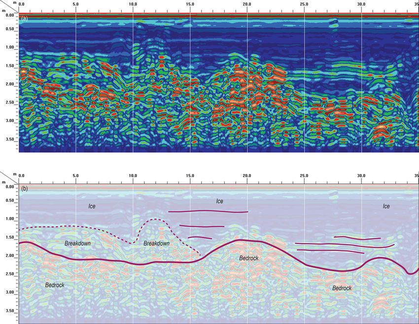
864                                                                          J. S. Munroe: First investigation of perennial ice

ice masses will be lost forever (Kern and Perşoiu, 2013; Veni        1. determine the origin, extent, and age of the ice in this
et al., 2014).                                                           cave;
   Despite the exciting potential of ice caves as paleocli-
                                                                      2. develop and interpret a stable-isotope record for this ice;
mate archives, these features remain an understudied com-
ponent of the cryosphere. Although an overview of ice caves           3. analyze and interpret the glaciochemistry of the ice.
in a variety of settings was presented more than 100 years
ago (Balch, 1900), most modern investigations of cave ice
have been conducted in a few focused areas, particularly the      2     Methods
Alps (e.g., Luetscher et al., 2005; May et al., 2011; Morard
                                                                  2.1    Field site
et al., 2010) and the mountains of Romania (e.g., Perşoiu
et al., 2011; Perşoiu and Pazdur, 2011). There, techniques       Fieldwork was conducted within Winter Wonderland Cave
for dating cave ice (e.g., Kern et al., 2009; Luetscher et al.,   in the Uinta Mountains of northeastern Utah, USA. Win-
2007; Spötl et al., 2014), interpreting stable-isotope records    ter Wonderland Cave (hereafter “WWC”) was discovered
in cave ice (e.g., Kern et al., 2011b; Perşoiu et al., 2011),    in 2012 and has an entrance at an elevation of 3140 m
and studying the glaciochemistry (e.g., Carey et al., 2019;       on a north-facing cliff. The cave is developed in the
Kern et al., 2011a) of cave ice have been developed over          Carboniferous-age Madison Limestone, a regionally exten-
the past several decades. Technologies such as environmen-        sive rock unit that in this area consists of fine- to coarse-
tal data loggers have simultaneously enabled investigation of     grained dolomite and limestone, with locally abundant nod-
micrometeorology in ice caves (e.g., Luetscher and Jeannin,       ules of chert (Bryant, 1992). The general location is pre-
2004b; Obleitner and Spötl, 2011), and geophysical tech-          sented in Fig. 1, but to preserve this fragile cave environment
niques such as ground-penetrating radar (GPR) have been           and the ice formations within it, the exact coordinates of the
employed to image ice stratigraphy (e.g., Behm and Haus-          cave entrance are withheld. The cave has a vertical extent of
mann, 2007; Colucci et al., 2016; Gómez Lende et al., 2016;       33 m and a mapped length of 245 m (Fig. 1c). The narrow en-
Hausmann and Behm, 2011). In general, however, these tech-        trance slopes down steeply ∼ 10 m to a roughly circular room
niques have been employed only on a limited basis elsewhere       (∼ 10 m diameter) with a high ceiling and flat floor of ice.
in the world. In North America, the ablation of subterranean      From this “Icicle Room” a narrow crack leads off to intersect
ice masses has been monitored in New Mexico (Dickfoss et          with the “Frozen Freeway”, a larger passage that forms the
al., 1997) as well as in lava tubes on the Big Island of Hawaii   main part of the cave. This steep-sided canyon, with walls up
(Pflitsch et al., 2016) and in California (Fuhrmann, 2007;        to 8 m high, developed along a vertical fracture bearing 160◦
Kern and Thomas, 2014). Seminal work on stable isotopes           (or 340◦ ). Similar steeply dipping fractures, at spacings rang-
in cave ice was conducted in the Canadian Rocky Moun-             ing from ∼ 20 to > 200 cm, are responsible for the porosity
tains (Lauriol and Clark, 1993; Yonge and MacDonald, 1999,        and permeability of the limestone host rock. The part of the
2014), and micrometeorology studies have been published           Frozen Freeway closer to the Icicle Room is a descending
on sites with (possibly) perennial ice in the northern Ap-        slope of breakdown derived from the cave ceiling. Beyond
palachian Mountains (Edenborn et al., 2012; Holmgren et al.,      this section, most of the floor of the Frozen Freeway is ice
2017).                                                            (Fig. 1c). The Frozen Freeway terminates in a wider section
   The most extensive investigation of a North American ice       with an ice floor called the “Skating Rink”. Beyond the Skat-
cave focused on Strickler Cavern, a site in the Lost River        ing Rink, the cave splits into two passages, both of which are
Range of Idaho (Munroe et al., 2018). That work documented        choked with rock debris. Strong air currents passing through
coexistence of firn ice and congelation ice with radiocarbon      these rock piles suggest the presence of considerable addi-
age control extending back ∼ 2000 years. Stable isotopes in       tional passage beyond the chokes. This air current has subli-
this ice were interpreted to record cooling temperatures lead-    mated the ice at the edge of the Skating Rink, producing an
ing into the Little Ice Age, and analysis of major and trace      exposure ∼ 2 m tall (Fig. 1c).
elements supported identification of a local component and           Fieldwork focused on documenting the temperature condi-
an exotic component of the overall dissolved load in the ice.     tions within WWC, determining the thickness of the peren-
   The project presented here applied the successful multi-       nial ice, gathering organic remains for radiocarbon dating,
disciplinary approach from Strickler Cavern (Munroe et al.,       and collecting ice samples for glaciochemical and isotopic
2018) to another cave containing ice of a different genesis.      analysis. Visits to WWC for this project were made on
In addition to radiocarbon dating and glaciochemical and          11 August 2016, 29 August 2018, and 19 August 2019.
isotopic analysis, a 2-year deployment of temperature data
loggers was incorporated to constrain cave meteorology, and       2.2    Cave temperature monitoring
GPR was employed to determine the thickness of the peren-
nial ice body. The primary objectives of the project were to      Three temperature data loggers (Onset Temp Pro v2) were
                                                                  deployed within the cave from August 2016 through Au-
                                                                  gust 2018 (Fig. 1c). Each logger was suspended from the

The Cryosphere, 15, 863–881, 2021                                                        https://doi.org/10.5194/tc-15-863-2021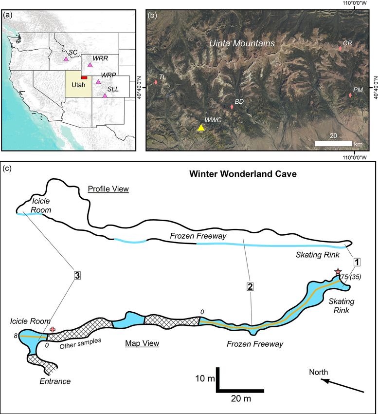
J. S. Munroe: First investigation of perennial ice                                                                                        865

Figure 1. Location map of the study area. (a) Western North America with US state outlines. The state of Utah is highlighted. The red box
denotes the location of the enlargement in panel (b). Other sites noted in the text are identified: Strickler Cavern (SC; Munroe et al., 2018),
Wind River Range (WRR; Naftz et al., 1996), White River Plateau (WRP; Anderson, 2012), San Luis Lake (SLL; Yuan et al., 2013). (b)
Enlargement of the Uinta Mountain region in USA National Agricultural Imagery Program (NAIP) natural color imagery. The yellow triangle
marks the location of Winter Wonderland Cave (WWC). Other sites noted in the text are identified: Trial Lake (TL) snowpack-monitoring site
and snow sampling site, Brown Duck (BD) snowpack-monitoring site, Pole Mountain (PM) snow sampling site, Chepeta remote automated
weather station (RAWS; CR). (c) Profile and map views of Winter Wonderland Cave simplified from mapping by David Herron, USDA
Forest Service. The cross-hatching pattern denotes breakdown, and the blue color denotes perennial ice. The locations of the cave entrance,
the Icicle Room, the Frozen Freeway, and the Skating Rink are noted. The orange lines mark the ground-penetrating radar transects. The
numbers 0 and 75 mark the start and end of the transect in the Frozen Freeway. Only the last 35 m of this transect are interpreted in the text.
The numbers 0 and 8 mark the start and end of the transect in the Icicle Room. The red star at the end of the Skating Rink is the exposure
described in the text. The red cross marks the exposure at the edge of the Icicle Room. “Other samples” highlights the region where additional
local ice samples were collected from between blocks of breakdown. The boxed numerals 1–3 identify the locations of the temperature data
loggers.

ceiling to measure temperature of the free air ∼ 30 cm away               downloaded into the proprietary Onset software Hoboware,
from the rock walls and ice surface. The loggers were set to              filtered to calculate daily mean values, and exported to a
record the temperature every hour. An additional logger was               spreadsheet for further analysis and plotting.
deployed within a solar-radiation shield outside the cave en-
trance to record ambient air temperatures. The temperature
data loggers were collected in late August 2018. Data were

https://doi.org/10.5194/tc-15-863-2021                                                              The Cryosphere, 15, 863–881, 2021
866                                                                        J. S. Munroe: First investigation of perennial ice

2.3   Ground-penetrating radar                                       Samples of rodent droppings were selected for AMS 14 C
                                                                  dating at NOSAMS (National Ocean Sciences Accelerator
To constrain the thickness of the ice, GPR surveys were con-      Mass Spectrometry facility) and ICA (International Chem-
ducted along the Frozen Freeway in 2019 following stan-           ical Analysis Inc.). Each was dried, weighed, and pho-
dard protocols (e.g. Hausmann and Behm, 2011). A shielded         tographed before submission. Resulting radiocarbon ages
400 MHz antenna and a GSSI SIR-3000 controller were used          were calibrated against the IntCal 20 calibration curve data
to collect the radar data. Before the survey, a transect was      (Reimer et al., 2020) in Oxcal 4.4. All of the samples yielded
established with measured points every 5 m. A mark was            multiple possible calibration ranges.
recorded in the GPR data each time the antenna passed one
of these points, which allowed the GPR results to be con-         2.5   Isotopic and glaciochemical analyses
verted to a physical horizontal scale. A shorter survey was
also conducted in the Icicle Room. In both locations, surveys     Ice samples were collected from existing exposures using
were conducted multiple times, in both directions. Gain set-      an approach similar to that employed in previous studies
tings were determined using an auto-gain procedure at the         (e.g., Carey et al., 2019). Using a hand-operated ice screw,
start of each transect to optimize the balance between detect-    a total of 84 samples were collected from the 2 m high expo-
ing stratigraphy in the ice and simultaneously imaging the        sure of ice at the rear of the Skating Rink (Fig. 2). Working
underlying ice–rock interface.                                    downward from the top, samples were collected at a spacing
   Data collected with the GPR were processed with Radan          of 2 cm for the first 150 cm and 5 cm for the bottom 50 cm.
7.0. Processing involved standard steps (e.g., Colucci et al.,    At each level, two holes were drilled side by side, and the
2016; Hausmann and Behm, 2011), including a time-zero             resulting ice cores were collected in 50 mL screw-top tubes.
correction to eliminate the impulse passing directly from         The first several centimeters of ice drilled out at each hole
the antenna to receiver (the direct wave); a full-pass back-      were discarded to avoid the possibility of meltwater contam-
ground removal to remove the surface wave; a finite impulse       ination near the ice surface (Kern et al., 2011a). Additional
response (FIR) stacking filter to remove airwave reflections      samples of ice were collected with the same method from
from the cave walls; an additional FIR filter to clip the band-   the Icicle Room as well as local exposures within the pile of
width between 300 and 700 MHz; an adaptive gain proce-            breakdown at the entrance to the Frozen Freeway (Fig. 1c).
dure to amplify faint, deeper reflectors; distance normaliza-     Samples of liquid water from pools on the Skating Rink were
tion to produce a scaled profile; and migration to remove         collected in 2018 and 2019 in 50 mL screw-top vials with no
hyperbolic reflectors produced by objects within the ice. A       head space.
dielectric permittivity of 3.15, typical of pure ice (Thom-          Ice samples were melted overnight and filtered to 0.2 µm
son et al., 2012) and corresponding to an average velocity of     the next day into new 15 mL tubes with no head space. These
∼ 0.16 m/ns, was used to convert two-way radar travel times       were stored at 4 ◦ C before analysis (< 48 h later) of δ 18 O and
to estimated depths below the surface of the ice. Because the     δD in a Los Gatos Research DLT-100 water isotope analyzer
focus was on determining the thickness of the ice, no attempt     with a CTC Analytics autosampler at Brigham Young Uni-
was made to account for the different permittivity of the un-     versity. Analysis followed standard procedures (e.g., Perşoiu
derlying bedrock.                                                 et al., 2011). Each sample was run 8 times, along with a set of
                                                                  three standards, which were calibrated against VSMOW (Vi-
2.4   Geochronology                                               enna Standard Mean Ocean Water). Precision of the resulting
                                                                  δ 18 O and δD measurements is ±0.2 ‰ and ±1.0 ‰, respec-
To constrain the age of the ice, rodent droppings within the      tively. Stable-isotope results were compared against values
ice were retrieved by angling an ice screw so that it inter-      for the location of WWC obtained from the Online Isotopes
sected with the dropping and raised it to the surface. This       in Precipitation Calculator (OIPC; http://waterisotopes.org,
technique was limited to droppings visible within the up-         last access: 12 February 2021).
per 15 cm of the ice, corresponding to the length of the ice         For glaciochemical analysis, remaining samples of melt-
screw. However, because the surface of the ice was locally        water were acidified with trace-element-grade nitric acid and
sublimated into a series of valleys and troughs with relief       stored at 4 ◦ C before analysis with a Thermo Fisher iCAP
of ∼ 30 cm, drilling in the base of the troughs permitted the     Qc inductively coupled plasma mass spectrometry (ICP-
retrieval of droppings from deeper levels beneath the origi-      MS) at Middlebury College following standard procedures
nal ice surface. Samples were collected along the length of       (e.g., Kern et al., 2011a). Each sample was run 3 times, with
the Frozen Freeway (Fig. 2); depths of these samples were         blanks and reference standards between every five samples.
estimated relative to the height of the nearest ridge on the      Samples were calibrated against a standard curve developed
sublimated ice surface (Table 1). An additional sample was        with five concentrations of an in-house standard based on Na-
collected from a depth of ∼ 75 cm below the ice surface in        tional Institute of Standards and Technology (NIST) Stan-
the Icicle Room, taking advantage of a vertical exposure of       dard Reference Material (SRM) 1643f and drift-corrected
ice eroded by air currents entering from the Frozen Freeway.      based on the reference standards.

The Cryosphere, 15, 863–881, 2021                                                      https://doi.org/10.5194/tc-15-863-2021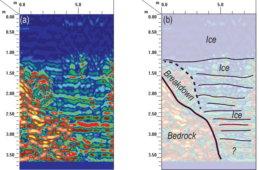
J. S. Munroe: First investigation of perennial ice                                                                                       867

Figure 2. Schematic illustrating the relationship between the Frozen Freeway, where most 14 C samples were collected from shallow depths
within the ice, and the taller exposure at the Skating Rink, where most samples for stable isotopes and glaciochemistry were collected. This
exposure reached to the cave ceiling, and the part projecting above the Frozen Freeway contained six visibly distinct layers. Intermediate
parts of this exposure were also visibly layered, with Layers 7 and 8 corresponding stratigraphically to the near-surface layers of the Frozen
Freeway, where the 14 C samples were collected. The bottom ice in this exposure did not appear to be layered, although it was difficult to
view this ice directly. The total height of the Skating Rink exposure is 2 m.

3     Results                                                            gers within the cave were approximately 0.5 ◦ C colder on
                                                                         1 May 2017 relative to 1 May 2018.
3.1    Temperature data loggers                                             Comparison of the records from all of the loggers indi-
                                                                         cates that when the outdoor temperature drops significantly
The temperature data loggers ran continuously during their               below 0 ◦ C, the Icicle Room begins to cool, followed a few
deployment, each recording 17 942 hourly measurements.                   days later by the loggers deeper within the cave (Fig. 4b). In
When plotted as time series, these data reveal a repeating               contrast, once the outdoor temperature stops cycling below
seasonal rhythm of temperatures within the cave as well as               0 ◦ C at the beginning of the summer, all loggers within the
air temperatures outside the cave entrance (Fig. 3). Temper-             cave exhibit greatly reduced short-term variability, and tem-
atures at all three positions within WWC remained continu-               peratures at all of them rise asymptotically toward their equi-
ously < 0 ◦ C. The coldest cave temperatures were recorded               librium value, which is reached later in the summer (Fig. 3).
by Logger 3 in the Icicle Room (average of −1.5 ◦ C), which              Equilibrium temperatures are warmest at Logger 3 (Skating
is closest to the cave entrance. There temperatures dropped              Rink, farthest back in the cave, Fig. 1c) and coldest at Logger
to below −8 ◦ C at times each winter, although typically tem-            1 in the Icicle Room near the cave entrance (Fig. 3).
peratures were closer to −4 ◦ C. The locations of Loggers 1                 Close inspection of the time series also reveals interesting
and 2 were warmer, −0.4 and −0.6 ◦ C, respectively (Fig. 4a).            short-term behavior at each of the logger sites. For instance,
The records from these loggers also exhibit a great degree of            air temperatures in the Icicle Room (Logger 3) exhibit tran-
similarity and are strongly correlated with one another (r 2 of          sient ∼ 1 d increases in air temperature during the summer
0.986, p = 0.000). The temperature difference between these              on several occasions (Fig. 4c and d). These are mirrored by
two loggers was lowest in the winter and greatest in the sum-            simultaneous but smaller amplitude decreases in temperature
mer.                                                                     at the loggers deeper within the cave (Fig. 4c and d). Notably,
   The record from the logger outside WWC indicates a mean               after each of these disturbances, temperatures return to their
annual air temperature of 2.3 ◦ C (Fig. 4a). The winter of               baseline values. Another observation is that in May 2017,
2016–2017 was colder than 2017–2018 (based on the av-                    the temperature at Logger 2 rose above the temperature at
erage temperature between 1 November and 1 May). Both                    Logger 1 for about 10 d, the only interval during the entire
winters had a similar absolute coldest temperature of around             deployment when this reversal occurred (Fig. 4c). Finally, in
−21 ◦ C. Winter 2017–2018 had a longer stretch of time be-               early June 2018, the temperature at Logger 3 abruptly rose
tween the first and last subzero temperatures, but the begin-            about half a degree and stayed elevated relative to the tem-
ning of this winter was relatively warm. As a result,
                                                   P winter              perature at Logger 2 for the rest of the summer (Fig. 4d).
2016–2017 recorded 950 freezing degree days ( (0 ◦ C −
daily mean)) in comparison with 766 during the winter of
2017–2018 (both calculated from 1 November through the
end of May). In response to this difference, the data log-

https://doi.org/10.5194/tc-15-863-2021                                                              The Cryosphere, 15, 863–881, 2021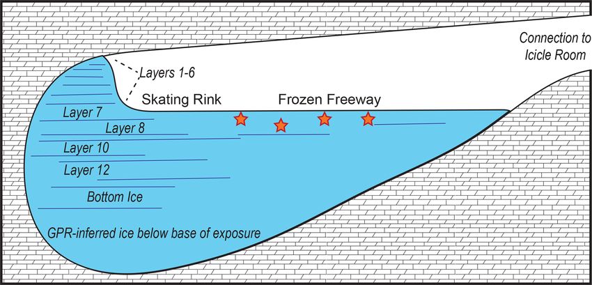
868                                                                                    J. S. Munroe: First investigation of perennial ice

Table 1. Radiocarbon dating results from Winter Wonderland Cave.

   Lab number      Lab           Sample      Location   Depth   Mass   14 C Age   ±     δ13C    Calibrated     Mean    Median   Note
                                                                                                range
   –               –             –           ∗            cm     mg          yr   yr       ‰    yr CE          yr CE    yr CE   –
   17O/0351        ICA           WW-20a      FF           20      60        40    30        –   1690–1730      1820      1830   –
                                                                                                (27.8 %),
                                                                                                1810–1920
                                                                                                (67.6 %)
   17O/0352        ICA           WW-20b      FF           20      22        50    30        –   1690–1730      1820      1830   –
                                                                                                (27.3 %),
                                                                                                1810–1920
                                                                                                (68.1 %)
   OS-128827       NOSAMS        WWC-IR-75   IR           75     200       145    15   −27.91   1670–1700      1810      1810   Composite
                                                                                                (14.7 %),
                                                                                                1720–1780
                                                                                                (22.7 %),
                                                                                                1790–1820
                                                                                                (10.2 %),
                                                                                                1830–1880
                                                                                                (26.7 %),
                                                                                                1900–1950
                                                                                                (20.9 %)
   OS-128826       NOSAMS        WWC-FF-45   FF           45      25       215    15   −26.71   1640–1680      1740      1770   –
                                                                                                (38.9 %),
                                                                                                1740–1800
                                                                                                (56.6 %)
   17O/0353        ICA           WW-30       FF           30      18       260    20        –   1520–1560      1650      1650   Single, intact
                                                                                                (12.1 %),
                                                                                                1630–1670
                                                                                                (74.3 %),
                                                                                                1780–1800
                                                                                                (9.0 %)
   OS-128804       NOSAMS        WWC-FF-5    FF            5      12       285    12   −27.26   1520–1560      1590      1560   –
                                                                                                (50.9 %),
                                                                                                1630–1660
                                                                                                (44.5 %)
   17O/0350        ICA           WW-15       FF           15      15         –     –        –   –                 –         –   –

∗ FF: Frozen Freeway; IR: Icicle Room.

3.2    Ground-penetrating radar                                             the strongest reflectors are found at depths greater than a me-
                                                                            ter below the ice surface.
                                                                               Along the entire length of the Frozen Freeway transect,
                                                                            a continuous reflector is discernible at depth, which likely
GPR surveys along the Frozen Freeway as well as in the Ici-
                                                                            represents the contact between the ice and the underlying
cle Room provided information about the thickness and in-
                                                                            bedrock (Fig. 5). In the Skating Rink, where the cave is
ternal stratigraphy of the ice. The survey in the Frozen Free-
                                                                            widest, and reflections from the walls were not an issue, the
way extended for 75 m through passage of varying widths
                                                                            maximum depth of this reflector (using a dielectric permit-
(Fig. 1c). Because the antenna was shielded, reflections from
                                                                            tivity of 3.15) is between 2 and 2.5 m below the current ice
the cave walls and ceiling were not an issue. However, in the
                                                                            surface.
narrowest sections (less than 2 m wide), overlapping reflec-
                                                                               The GPR transect in the Icicle Room spanned a length of
tions from the cave walls beneath the ice surface made it dif-
                                                                            8 m. Results imaged layered ice superimposed on a sloping
ficult to identify consistent stratigraphy in the ice. Nonethe-
                                                                            bedrock surface locally mantled by blocks of cave break-
less, in the 35 m spanning the wider sections, such as the
                                                                            down (Fig. 6). As in the Frozen Freeway, the upper 1 m of this
Skating Rink, clear stratigraphic details within the ice are
                                                                            ice exhibits only faint laminations; however below a depth of
apparent in the radar data (Fig. 5). These take the form of
                                                                            ∼ 1 m the strength of the reflectors defining these lamina-
subparallel bands at various depths, which are laterally con-
                                                                            tions increases markedly. Based on the pattern of these par-
sistent over several meters. There is a general trend of less
                                                                            allel reflectors and their relationship with the sub-adjacent,
pronounced reflectors in shallower parts of the ice, whereas

The Cryosphere, 15, 863–881, 2021                                                                   https://doi.org/10.5194/tc-15-863-2021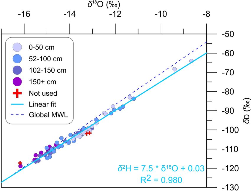
J. S. Munroe: First investigation of perennial ice 869
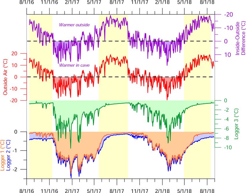
Figure 3. Temperature records from data loggers deployed in Winter Wonderland Cave from August 2016 through August 2018. Logger 1
was at the Skating Rink, Logger 2 along the Frozen Freeway, and Logger 3 in the Icicle Room (Fig. 1c). Outside air temperature was recorded
by a logger in a solar-radiation shield outside the cave entrance. Yellow shading highlights the summer periods, when cave ventilation is
greatly reduced. The purple time series at the top displays the difference between the temperature at Logger 1 and the temperature outside the
cave; note the inverted axis. Time series from loggers within the cave are filled below 0 ◦ C. Dashed black lines highlight 0 ◦ C on the outside
air and the temperature difference plots.
higher-intensity reflectors from the bedrock, the maximum posures of ice in and near the Icicle Room were analyzed
ice thickness in the Icicle Room, again assuming a dielectric successfully for δ 18 O and δD. Overall, values of both iso-
permittivity of 3.15, may exceed 3 m (Fig. 6). topes are notably depleted relative to VSMOW, with an aver-
age δ 18 O of −14.0 and δD of −104 (Table 2). Minimum and
3.3 Radiocarbon dating maximum values of δ 18 O are −17.6 ‰ and −8.7 ‰ and for
δD are −125 ‰ and −64 ‰. Overall, values of δ 18 O and δD
Seven samples of rodent droppings collected from WWC are strongly and linearly correlated with one another (r 2 of
were submitted for AMS radiocarbon dating. Six of these 0.957).
samples were successfully dated, yielding ages from 40 to Given the wide range of isotope values in the samples from
285 radiocarbon years, corresponding to median calibrated the Skating Rink exposure, a three-step screening was con-
ages from CE 1830 to CE 1560 (Table 1, Fig. 7). The old- ducted to identify outliers. First, values of d-excess in parts
est of these samples has a 2σ calibration range that extends per thousand were calculated as d-excess = δD − (8 × δ 18 O)
back to CE 1520. Three of the samples have 2σ calibration (Dansgaard, 1964). Second, because the distribution of the
ranges that extend, with low probability, into the 20th century original data was not normal as revealed by a Shapiro–Wilk
(Fig. 7). Overall, the estimated depths of the samples below test (p = 0.014), the values were log-transformed. Third, val-
the local ice surface have no relationship with their ages. The ues > 2 standard deviations away from the mean were tagged
oldest sample (WWC-FF-5) was from the shallowest depth as outliers. This process identified three samples: two with
(5 cm). On the other hand, two samples obtained near one an- anomalously low values of d-excess and one with an unusu-
other from the same depth (WW-20a and WW-20b) yielded ally high value (Fig. 8). These samples were removed from
identical ages. further consideration, leaving 81 samples from this exposure.
On a plot of δ 18 O vs. δD, these 81 samples from the Skat-
3.4 Stable isotopes
ing Rink exposure plot parallel to and generally slightly be-
A total of 94 samples collected from the continuous exposure low the global meteoric waterline (Fig. 8). A linear regres-
at the back of the Skating Rink (Fig. 2) and from isolated ex-
https://doi.org/10.5194/tc-15-863-2021 The Cryosphere, 15, 863–881, 2021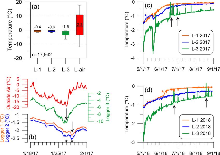
870                                                                                                          J. S. Munroe: First investigation of perennial ice

Figure 4. Details of temperature records from Winter Wonderland Cave. (a) Box-and-whisker plot showing the distribution of temperature
measurements at each of the three loggers (L-1 through L-3) as well as outside the cave. (b) Detailed view of temperature records from
late January 2017. A notable low point in temperature outside the cave was mirrored immediately by a temperature drop within the Icicle
Room, recorded by Logger 3 on 27 January (star). A corresponding drop in the temperature deeper in the cave was recorded 2 d later (second
black arrow and star), supporting the theory that cold air enters through the Icicle Room in winter. (c, d) Temperatures during the summer
of 2017 (c) and in the summer of 2018 (d) at the loggers within the cave. The black arrows highlight examples of transient warming in the
Icicle Room that were not observed deeper in the cave. The blue star in (c) marks an interval in early May, when the temperature at Logger
2 in the Frozen Freeway briefly rose above the temperature of Logger 1 at the Skating Rink. The orange star in (d) highlights a dramatic,
permanent increase in temperature at Logger 1, interpreted to represent the arrival of meltwater at the back of the cave in 2018.

Table 2. Stable-isotope results for Winter Wonderland Cave.

               Avg δ 18 O   SD δ 18 O   Avg δD     SD δD     d-excess   SD d-excess     Slope    Intercept    n       r2   Altered?    Estimated     Estimated   Summer precipitation
                                                                                                                                                                   fraction (fSummer)
                      ‰           ‰          ‰         ‰           ‰              ‰         –          ‰      –        –          –         δ 18 O         δD                       –
 Layer 1          −11.4             –      −83          –         7.9               –       –          –      1        –          –        −11.4         −83                    0.71
 Layer 2           −9.0           0.5      −66          3         6.0             1.2    5.76      −14.2      2    1.000        Yes        −10.5         −75                    0.79
 Layer 3          −12.1             –      −88          –         9.0               –       –          –      1        –          –        −12.1         −88                    0.65
 Layer 4          −12.6           0.2      −93          3         7.6             1.3   13.70       79.2      3    0.965        Yes        −12.4         −90                    0.62
 Layer 5          −13.3           0.1     −100          1         6.0             0.3    9.17       21.5      3    0.924        Yes        −10.0         −70                    0.83
 Layer 6          −13.5           0.2     −102          2         5.7             0.4    7.64        0.9     10    0.949        No         −13.5        −102                    0.53
 Layer 7          −13.6           0.6     −103          4         5.5             1.4    5.98      −21.9     10    0.961        Yes        −15.2        −112                    0.38
 Layer 8          −12.7           1.3      −94          8         7.4             2.0    6.51      −11.6      8    0.996        Yes        −13.8        −100                    0.51
 Layer 9          −14.0           0.9     −105          6         7.1             2.0    6.88       −8.5      7    0.921        Yes        −15.5        −115                    0.35
 Layer 10         −14.9           0.0     −113          2         5.5             0.7   12.06       65.0      3    0.959        Yes        −14.0        −105                    0.48
 Layer 11         −13.6           0.2     −102          2         6.9             0.8    6.47      −13.9     11    0.826        Yes        −14.8        −110                    0.42
 Layer 12         −14.6           0.4     −110          3         7.3             0.4    8.01        7.4      9    0.985        No         −14.6        −110                    0.43
 Layer 13         −15.1           0.3     −114          3         7.3             0.6    8.03        7.7      6    0.956        No         −15.1        −114                    0.39
 Bottom           −15.4           0.5     −113          4         9.9             1.1    6.69      −10.3     10    0.940        Yes        −14.8        −107                    0.42
 Mean all         −14.0           1.4     −104         10         7.7             2.5    7.03        −5.8    94    0.957          –             –            –                     –
 Mean SR∗         −13.8           1.3     −103         10         7.1             1.7    7.40        −1.3    84    0.976          –             –            –                  0.54
 Mean IR∗         −15.2           1.4     −109         11        13.0             1.3    7.36         3.2    10    0.994          –             –            –                     –

∗ SR: Skating Rink; IR: Icicle Room. The δ 18 O and δ D estimations were determined from the intersection of the line fit to the data with the meteoric water line

The Cryosphere, 15, 863–881, 2021                                                                                          https://doi.org/10.5194/tc-15-863-2021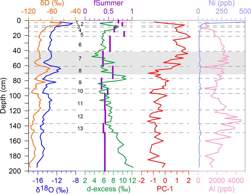
J. S. Munroe: First investigation of perennial ice                                                                                       871

Figure 5. Results of a ground-penetrating-radar (GPR) survey along the Frozen Freeway. (a) Uninterpreted GPR data for half of the full
survey length (35 m out of 75 m), with the back of the cave on the right. Vertical white lines mark measured points every 5 m used for scaling
the GPR survey. (b) Interpretation of the GPR survey shown in (a). The bedrock surface is represented by an irregular but laterally continuous
contact. More isolated and discontinuous zones of high-amplitude reflectors above this contactor interpreted as piles of breakdown. Ice
beneath the Skating Rink, between 20 and 35 m along the transect, reaches a maximum thickness of nearly 2.5 m. Ice along the Frozen
Freeway, between 0 and 20 m, has a maximum thickness of ∼ 2 m. Horizontal lines within the ice are interpreted as stratigraphic layers.

sion through the 81 samples from the continuous exposure                 However, isotopic values do not always change appreciably
has a slope of 7.5 and y intercept of 0.03 (r 2 of 0.980).               across these layer boundaries. For example, δ 18 O and δD rise
   Plotting values of δ 18 O and δD vs. depth in the 2 m high            steadily through Layer 5, continuing a trend that spans from
exposure reveals short-term variability superimposed over a              Layers 4 through 6 (Fig. 9). The boundary between Layers
longer trend (Fig. 9). In general, deeper samples have more              10 and 11 appears to be the only instance in which a visible
negative δ values. Samples with the highest values were col-             boundary coincides with a major change in isotope values (a
lected from within a few centimeters of the cave ceiling. The            shift in δ 18 O of 1.2 ‰ and δD of 12 ‰).
overall trend in d-excess runs generally contrary to δ 18 O and
δD, with higher values in deeper ice (Fig. 9).                           3.5    Glaciochemistry
   In the field, the upper 1.5 m of this exposure, which was
more accessible, was visibly stratified, with thin layers of             A total of 13 major and trace elements were detectable
fine carbonate precipitates defining boundaries between 13               in ice samples analyzed from the exposure at the Skating
discernible layers (Fig. 2). Similar layers were not noticed in          Rink. Ranked in order from most to least abundant they are
the bottom 50 cm of the exposure; however this may reflect               Ca > Al > Mg > K > Na > P > Si > Ni > Ti > Ba > Sr > Mn
the fact that it was difficult to view the bottom of the exposure        > Rb (Fig. 10). Peak abundances of calcium are
head-on. Some of these layers, which range from 2 to more                ∼ 20 000 ppb, and Al, Mg, K, and Na are all detectable
than 20 cm thick, correspond with variations in δ 18 O and δD            in some samples at concentrations above 1000 ppb. Rubid-
(Fig. 9). For instance, δ values are notably higher in Layer 2,          ium is the least abundant detectable element, generally with
with δ 18 O up to −8.7 ‰. Similarly, Layer 8 and the central             a mean of 0.5 ppb. P, Si, and Sr were not detectable in some
part of Layer 9 both contain ice with relatively high δ values.          samples. A principal component analysis applying a varimax

https://doi.org/10.5194/tc-15-863-2021                                                              The Cryosphere, 15, 863–881, 2021
872                                                                                  J. S. Munroe: First investigation of perennial ice

Figure 6. Results of an 8 m long ground-penetrating-radar (GPR) survey across the Icicle Room, presenting uninterpreted (a) and inter-
preted (b) data. From the surface to a depth of ∼ 1 m, the ice is only faintly stratified, whereas below that depth the ice contains increasingly
prominent radar reflectors. The steeply sloping bedrock surface is defined on the left side of the transect, mantled in places by breakdown.
The maximum thickness of ice here is unclear, but it may be in excess of the 3.5 m penetrated by the 400 MHz GPR system.

Figure 7. Calibration ranges from the IntCal 20 calibration curve
for radiocarbon dates obtained from Winter Wonderland Cave.
Sample labels correspond with Table 1. Circles mark the mean cali-
brated age for each sample; diamonds denote the median age. Both           Figure 8. Plot of δ 18 O vs. δD for ice samples from the Skating
are labeled in years CE.                                                   Rink exposure (Fig. 1c). Samples are color-coded to highlight their
                                                                           depth below the top of the exposure. Three samples identified as
                                                                           outliers and discarded from the dataset are marked with red crosses.
                                                                           The solid light-blue line represents a linear regression through the
rotation to log-transformed values of Ca, Al, Mg, K, Na, Ti,               remaining 81 samples, and the equation for this line is presented in
Ba, Mn, and Rb (removing P, Si, and Sr, which were not                     the lower right corner. The dashed blue line is the global meteoric
detectable in all samples) loads all elements except Al and                waterline (Craig, 1961).
Ni on the first principal component (PC-1) at values from
0.763 to 0.890. These elements follow a consistent pattern
of generally low values in the bottom half of the exposure,
rising values between ∼ 100 and 50 cm depth, and notably                   (0.891), and Al is strongly and negatively correlated with
elevated values in the uppermost 50 cm (Fig. 9). In contrast,              PC-3 (−0.827). Nickel has general low and stable values
Ni exhibits the strongest positive correlation with PC-2                   until the uppermost sample, whereas Al abundance is high

The Cryosphere, 15, 863–881, 2021                                                                 https://doi.org/10.5194/tc-15-863-2021
J. S. Munroe: First investigation of perennial ice 873
Figure 10. Box-and-whisker plot presenting the abundance of de-
tectable elements in samples from the Skating Rink exposure, ar-
ranged from most to least abundant. Central lines represent median
Figure 9. Composite plot of values measured in the Skating Rink
values, boxes represent interquartile range, whiskers represent in-
plot against depth below the top of the exposure. Values of δ 18 O
terquartile range ×1.5, and circles represent outliers.
vs. δD are shown in the first column. The d-excess and the recon-
structed fraction of summer monsoonal water in the ice are shown
in the second column. The first principal component determined for
the glaciochemistry result is displayed in the third column. The two As illustrated in Fig. 3, cold air enters the Icicle Room (Log-
elements which do not fit into PC-1, Al, and Ni are shown in the ger 3) whenever the outside air temperature drops notably
fourth column. Dashed horizontal lines mark visible boundaries ob- below the temperature in the cave. If cold temperatures out-
served in the exposure. From top to bottom, these layers are num- side are maintained for more than a few days, this cold pulse
bered 1 through 13. The shaded gray region marks the approximate penetrates deep enough into the cave to be recorded by Log-
depth from which the radiocarbon ages along the Frozen Freeway ger 2 in the Frozen Freeway and Logger 1 at the Skating Rink
were obtained. The ice in this depth range likely dates to between (Fig. 4b). Although the slight downhill slope of the entrance
CE 1560 and 1830; deeper ice is older.
passage leading to the main part of the cave would alone en-
courage the entry of dense cold air in winter, the extreme
narrowness of the actual cave entrance (< 25 cm) combined
between 125 and 150 cm and again around a depth of 50 cm
with the observation of a substantial draft flowing through the
(Fig. 9).
cave during each field visit suggests that a connection exists
Similar elemental abundances were measured in the ice
between the currently accessible end of WWC and the sur-
samples collected between the Frozen Freeway and the Ici-
face of the plateau ∼ 100 m above the cave. This conduit acts
cle Room. Calcium is again the most abundant element, with
as a chimney, allowing relatively warm air within the cave to
an average concentration of 4850 ppm, and Rb is the least
rise towards the surface in the winter (Balch, 1900; Luetscher
abundant (< 1 ppm). Mean abundances for all elements in
and Jeannin, 2004b; Thury, 1861). This air is replaced by
these samples are strongly correlated with those measured
cold air flowing in through the cave entrance into the Ici-
for the Skating Rink exposure (r 2 of 0.945). Unlike in the
cle Room, refrigerating the cave interior throughout the win-
exposure at the Skating Rink, there is no obvious trend in
ter. In contrast, during the summer, there is a minor reversal
abundance in these samples. However, because they were
of this pattern as cold air within the cave flows out through
collected from isolated locations where ice was locally visi-
the entrance, replaced by warm air penetrating downward
ble between blocks of breakdown, their relationship with one
through the hypothesized connection between the cave and
another is unclear, and it may be inappropriate to consider
the plateau surface. However, because the entrance of the
them parts of a stratigraphic sequence.
cave is ∼ 15 m higher than the Frozen Freeway (Fig. 1c), it is
not possible for all of the dense cold air to be evacuated from
4 Discussion the cave in the summer. As a result, the interior of WWC is
disproportionately impacted by cold air in winter and is rela-
4.1 Origin, extent, and age of the ice tively unaffected by summer warmth.
Occasionally, during the summer months the temperature
The data loggers that recorded air temperatures between in the Icicle Room abruptly jumps ∼ 1 ◦ C before returning to
2016 and 2018 provide a clear explanation for why peren- baseline levels (Fig. 4c and d). This shift is accompanied by a
nial subzero conditions are maintained inside WWC despite minor temperature decrease at the loggers deeper in the cave.
a mean annual temperature of +2.3 ◦ C outside the entrance. This pattern indicates that some process brings relatively
https://doi.org/10.5194/tc-15-863-2021 The Cryosphere, 15, 863–881, 2021874 J. S. Munroe: First investigation of perennial ice warm outside air into the Icicle Room, displacing colder air could have maintained the slightly warmer temperatures rel- deeper into the cave but not for long enough to have a last- ative to Logger 2. Snowpack-monitoring sites at Trial Lake ing impact on the overall temperature distribution. Compari- and Brown Duck, at similar locations, elsewhere in the south- son of the logger records with meteorological data from the western Uinta Mountains (Fig. 1b) rapidly lost the majority Chepeta RAWS (remote automated weather station) 60 km to of their snow water equivalent in May 2018. This offset sug- the east (Fig. 1b) at a slightly higher elevation (3680 m) indi- gests that it requires ∼ 1–2 weeks for meltwater to transit cates that each of these transient temperature increases was from the plateau surface to the cave. associated with wind from 320 to 340◦ at velocities greater Results from the GPR surveys indicate that the ice form- than 15 m/s. Given the orientation of the cave entrance, this ing the floor of the Frozen Freeway is generally from 1 to azimuth is perfectly aligned to push relatively warm outside ∼ 2.5 m thick and has accumulated over an uneven surface of air through the cave entrance, temporarily warming the Icicle bedrock and blocks of breakdown (Fig. 5). The 2 m high ex- Room and displacing cold air deeper into the cave. However, posure of ice at the edge of the Skating Rink starts ∼ 45 cm because the general airflow is outward during the summer, as above the floor of the Frozen Freeway, exploiting remnant soon as the wind direction or velocity changes, and warm air ice layers reaching to the cave ceiling that have not been re- is no longer forced into the cave, the pattern reverses, and the moved by sublimation (Fig. 2). Given the assumed dielectric Icicle Room cools down again. permittivity, therefore, it is possible that as much as a meter Given the distribution of ice and the lack of ice stalactites of additional ice exists below the deepest stratigraphic level or stalagmites along the Frozen Freeway, it appears that the accessible in this exposure. Similarly, in the Icicle Room, an water responsible for the ice in WWC entered through the ice thickness possibly in excess of 3 m was imaged (Fig. 6). boulder-choked constrictions in the rear of the cave as well In both locations, the tendency of the upper ∼ 1 m of ice as through the entrance into the Icicle Room. Because there to exhibit reduced stratigraphic layering compared with the are no streams or lakes in the landscape above the cave, this deeper ice may reflect a greater presence of mineral precip- water is likely derived from infiltrating precipitation. Further- itates, dust, or organic matter concentrated at specific levels more, given the climate at this location, much of this water within the deeper ice. is likely related to the melting of winter snowpack in late Determining the age of cave ice deposit is rarely straight- spring. This rapid melt produces a pulse of water that pene- forward, and the situation in WWC is no different. Compared trates downward through the epikarst to reach the back of the with a sag-type cave in which snow and organic matter accu- cave, perhaps following the conduit that allows cave air to mulate in a vertical shaft (e.g., Munroe et al., 2018; Spötl rise toward the surface in the winter. Snowmelt on the north- et al., 2014), the interior of WWC is relatively devoid of or- facing cliff above the cave entrance can enter the Icicle Room ganic matter. On the other hand, the radiocarbon-dated rodent directly. It is also possible that intense summer rainstorms droppings do provide important age constraints (Fig. 7). Be- may deliver water to the plateau above WWC in quantities cause these samples were collected from the upper layers of sufficient to reach the cave. Either way, this water freezes the ice deposit (Fig. 2), they provide minimum limits on the upon entering the subzero cave interior, incrementally adding age of the ice, suggesting that most of the ice accumulated a new layer to the perennial ice deposit. Given the hypoth- before ∼ CE 1830. esized conduit linking the cave to the surface, this model of ventilation for maintenance of freezing temperatures, and 4.2 Paleoclimate implications the apparent formation of ice from inflowing water, WWC can be classified as a “dynamic cave with congelation ice” The overall pattern in these data is that the deep ice is more (Luetscher and Jeannin, 2004a). depleted in heavy isotopes relative to VSMOW, whereas Winter Wonderland Cave was not visited during the sum- stratigraphically higher ice is less depleted (Fig. 9). This mer of 2017, so it is unknown whether water entered the cave trend indicates a long-term change in the isotopic compo- that year. However, in August 2018, liquid water and new sition of the water entering WWC. Air temperature exerts a ice were noticed at the Skating Rink and along parts of the well-documented effect on isotopic values of precipitation, Frozen Freeway. The temperature data logger from the Skat- with a lower temperature of condensation corresponding to ing Rink (Logger 1) recorded a ∼ 1 ◦ C increase in tempera- lower values of δ 18 O and δD (Dansgaard, 1964). There- ture during the first week of June 2018 (Fig. 4d). In contrast fore, one possible interpretation is that average air tempera- to the summer temperature increases in the Icicle Room, this tures increased over the time period represented by the Skat- temperature rise was long-lasting: during the weeks leading ing Rink exposure. However, given the relationship between up to this point the temperatures at Logger 1 and Logger monthly average temperature and estimated δ 18 O for precip- 2 were identical, yet after this point, Logger 1 at the Skat- itation at the Brown Duck snowpack telemetry (SNOTEL) ing Rink remained ∼ 1 ◦ C warmer than Logger 2. The ar- site (Fig. 1b), the difference between the lowest (−16.2 ‰) rival of relatively warm meltwater to the back of the cave and highest δ values (−8 ‰) in samples from this exposure at this time could explain the abruptness of this temperature would correspond to a temperature change of approximately jump, and the slow release of latent heat as this water froze 11 ◦ C. This result exceeds the temperature difference be- The Cryosphere, 15, 863–881, 2021 https://doi.org/10.5194/tc-15-863-2021
J. S. Munroe: First investigation of perennial ice                                                                              875

tween full-glacial and modern conditions in the Uinta and          ter collected from the Skating Rink surface in August 2019,
Wasatch mountains determined from numerical modeling of            indicating that the water collected in the cave that summer
paleoglaciers (Laabs et al., 2006; Quirk et al., 2018, 2020).      was a mixture of winter snowmelt and isotopically heavier
It is difficult to imagine that the ice in WWC is residual from    summer rain.
the last glaciation, which reached its maximum in this area           With this insight, a linear mixing model was constructed to
at 18–20 ka (Laabs et al., 2009; Quirk et al., 2020); thus the     predict the δ 18 O value of water comprised of varying propor-
measured changes in the isotopic values are unlikely to be         tions of two end-members: snowmelt (at −19.6 ‰) and mon-
solely a function of temperature.                                  soonal rain (−8 ‰). This model suggests that the water col-
    A more plausible interpretation is that the isotopic vari-     lected from pools on the surface of the Skating Rink in late
ability reflects changes in the relative abundance of seasonal     summer 2019 was a mixture of 88 % winter snowmelt and
precipitation over WWC. Under the modern climate, the              12 % summer rain. This estimate of the summer component
Uinta Mountains are influenced by two distinct precipitation       in this sample is a minimum because the water had already
patterns strongly linked to specific seasons. Storms penetrat-     begun to freeze beneath a lid of ice, which would drive δ 18 O
ing inland from the Pacific Ocean produce a peak of precip-        in a more negative direction in the remaining water (Jouzel
itation during December, January, and February (Mitchell,          and Souchez, 1982; Perşoiu et al., 2011). Nonetheless, the
1976). By virtue of the cold winter air temperatures and the       value of δ 18 O in the modern water is more negative than any
long transport pathway for this moisture passing over multi-       of the analyzed ice samples, indicating either that this water
ple mountain ranges, this precipitation has notably low δ 18 O     contained a lower fraction of summer rain than the ice sam-
and δD values. In contrast, during the summer, primarily in        ples or that the snowmelt pulse in 2019 was unusually large.
August, moisture with relatively higher isotopic values is de-        Applying this mixing model to the ice samples requires
livered from the south by the North American Monsoon cir-          an assessment of whether the isotope values in the ice re-
culation (Metcalfe et al., 2015; Ropelewski et al., 2005). Cor-    flect those of the original precipitation or if they have been
respondingly, the Online Isotopes in Precipitation Calcula-        altered during freezing. In this regard it is notable that the ice
tor predicts that the location of Winter Wonderland Cave re-       in WWC is seen in vertical exposures to consist of visually
ceives precipitation with δ 18 O around −23 ‰ in winter and        distinct layers from < 5 to ∼ 20 cm thick, delineated by min-
around −8 ‰ in August.                                             eral precipitates and changes in bubble density (Fig. 2). Lay-
    The rapid 1 ◦ C increase in air temperature recorded by the    ering on a similar scale is also resolvable in the GPR results
logger at the Skating Rink in early June 2018 is a likely signal   (Figs. 5 and 6). If these layers were constructed through the
for the arrival of snowmelt at the beginning of that summer        incremental additions of thin films of water, then the mineral
(Fig. 4d). However, liquid water was still present at the Skat-    precipitates defining the visible layer boundaries could have
ing Rink more than 2 months later on 29 August 2018. Sim-          formed in response to sublimation that lowered the ice sur-
ilarly, although there is no temperature record for the sum-       face, creating a lag of material that was originally included
mer of 2019, liquid water was again observed at the Skating        in the ice. Alternatively, the visible layers may have formed
Rink on 19 August 2019. Assuming that the meltwater pulse          through slow, closed-system freezing of pools of water with
usually arrives at the beginning of the summer, matching the       a depth equivalent to the resulting layer thickness. Mineral
annual timing of snowmelt, the persistence of a thin layer         precipitates would have formed within each pool as the float-
(centimeter-scale) of liquid water in subzero conditions for       ing ice thickened downward, concentrating the residual liq-
multiple months is improbable. Therefore it is likely that ad-     uid water. Ice formed by these two mechanisms are termed
ditional water entered the cave later in the summers of 2018       “floor ice” and “lake ice”, respectively (Perşoiu et al., 2011).
and 2019, after the main snowmelt pulse. This summer water            Downward freezing of a layer of water beneath a thicken-
would most conceivably reflect the monsoonal precipitation         ing lid of ice will result in ice that is sequentially more de-
that dominates in August. In this model, therefore, the water      pleted in heavy isotopes at depth as the heavier 18 O and deu-
forming ice in WWC represents an integrated snowpack sig-          terium are preferentially incorporated into the early-formed
nal that is augmented by some amount of isotopically heavier       ice at the surface (Citterio et al., 2004b; Persoiu and Paz-
summer precipitation.                                              dur, 2011; Souchez and Jouzel, 1984). Thus, plotting δ 18 O
    The isotopic composition of the snowmelt directly above        and δD vs. depth and highlighting the locations of visually
WWC is unknown. However, fully integrated snowpack sam-            identified layer boundaries were employed to determine the
ples collected at the elevation of the plateau above the cave      likely origin of the different ice layers. When plotted this way
at Pole Mountain ∼ 50 km eastward along the southern flank         (Fig. 9), several layers exhibit trends of increasing isotope
of the Uinta Mountains in late March 2019 had an average           depletion with depth; however these differences are generally
δ 18 O of −18.9 ‰ (Fig. 1b). Similar full-snowpack samples         < 1 ‰ for δ 18 O from top to bottom in a given layer. The ex-
collected at the same elevation in early April 2019 at Trial       ception is Layer 8, where δ 18 O falls from −12 ‰ to −15 ‰
Lake ∼ 25 km northwest of WWC had an average δ 18 O of             over a layer thickness of 14 cm. Previous work has shown
−20.3 ‰ (Fig. 1b). The mean of all these values (−19.6 ‰)          that a top-to-bottom offset in δ 18 O of ∼ 4 ‰ occurs within
is lower than the value of −18.2 ‰ for two samples of wa-          5 to 10 cm thick layers of lake ice in a well-studied Roma-

https://doi.org/10.5194/tc-15-863-2021                                                      The Cryosphere, 15, 863–881, 2021
876 J. S. Munroe: First investigation of perennial ice nian ice cave (Perşoiu et al., 2011; Perşoiu and Pazdur, 2011). data points, creating uncertainty in its regression slope that With this observation as a reference point, Layer 8 in WWC carries over into the estimate of original water composition. likely formed through closed-system freezing of a thick layer Layer 7 contains two sets of isotopic values, a constant upper of water, and it is possible that this process slightly impacted half and a lower half with a pronounced negative excursion some other layers as well. (Fig. 9), implying that the suite of samples collected may Another way to evaluate the likelihood that ice formed have inadvertently spanned two layers separated by a con- through closed- or open-system freezing is to plot δ 18 O vs. tact that went unnoticed in the field. An obvious limitation is δD from an individual layer and assess whether the values that this simple model assumes that the isotopic composition align with the (local) meteoric waterline, indicating floor ice, of snowmelt and monsoonal precipitation was constant over or with a lower “freezing slope”, indicative of more exten- time. It also assumes that the interpolated isotopic value for sive fractionation, typical of lake ice (Jouzel and Souchez, August precipitation from the OPIC is accurate and that the 1982; Perşoiu et al., 2011). When arranged this way, sets snowpack samples from 2019 adequately represent the com- of samples (n ≥ 3) defining individual layers in the Skating position of the snow on the plateau above WWC. Nonethe- Rink exposure have slopes from 6.0 to 13.7 (Table 2). Lay- less, even with these considerations, it is notable that the rel- ers 6, 12, and 13 have slopes that are close to the meteoric ative importance of winter and summer precipitation appears waterline. The isotopic measurements in these layers, there- to have changed at this location over time. fore, likely record the composition of the original meltwater The radiocarbon-dated organic remains were collected with fidelity. In contrast, Layers 7, 9, and 11 and the bottom within the uppermost layers of ice forming the floor of the ice have lower slopes, suggesting more extensive fraction- Frozen Freeway, which corresponds to Layers 7 and 8 in the ation during freezing. The slopes of Layers 4, 5, and 10 are Skating Rink exposure (Figs. 2 and 9). This relationship al- quite high (> 9), although they were determined for just three lows the exposure to be divided broadly into a lower part, points. Previous work has demonstrated that isotopic compo- where the ice apparently accumulated prior to the 1800s, and sition of the original water can be found at the intersection of an upper part (Layers 1 through 6), which accumulated more a line fit to the δ 18 O and δD measurements for an individual recently. The lower layers, therefore, correspond with the in- ice layer and the meteoric waterline (Jouzel and Souchez, terval of generally cooler temperatures in the Northern Hemi- 1982; Perşoiu et al., 2011). Applying this approach yields sphere referred to as the Little Ice Age (Grove, 1988). The estimates of original δ 18 O and δD values for the layers that reconstructed summer water content of this ice varied in a appear to have fractionated extensively during closed-system narrow range between 40 % and 50 %, suggesting relatively freezing (Table 2). consistent conditions under which the snowmelt pulse and Two cautions must be noted when considering this anal- summer monsoon contributed roughly equal amounts of wa- ysis. First, samples were not collected continuously through ter to the cave. After this time, summer water began to exert the exposure; they were spaced 2 cm (for the upper part) and a greater control over the isotopic composition of the ice. 5 cm (for the lower part) apart. As a result, not all ice was Records of δ 18 O from lake sediments on the White River sampled, and the isotopic composition of the ultimate top Plateau in northwestern Colorado (Fig. 1a) suggest that win- and bottom ice in a given layer is unknown. Second, pre- ters during the Little Ice Age were notably snowy, with snow- vious work has noted that kinetic effects during rapid freez- fall making up the greatest fraction of annual precipitation at ing can cause deviations from the freezing slope (Perşoiu et any time during the Holocene (Anderson, 2012). After that al., 2011). Based on relationships between δD and d-excess, time, snowfall became less important. A similar pattern is kinetic effects likely played a role in the formation of at seen in multiproxy lacustrine records from San Luis Lake least some layers in the Skating Rink exposure. Nonetheless, (Fig. 1a) in southern Colorado (Yuan et al., 2013). The sug- with these considerations in mind, estimated isotopic com- gestion that water derived from the melting of winter snow positions of the original water obtained from the intersection contributed to a greater fraction of the ice forming in WWC of the freezing slope and meteoric waterline were combined during the Little Ice Age is consistent with these other re- with the average isotopic values for layers that apparently did gional hydroclimate records. An additional point of refer- not fractionate greatly, based on downward trends in isotope ence is provided by isotope measurements in a glacier ice values and δ 18 O vs. δD slopes. core from the Wind River Mountains (Fig. 1a), ∼ 400 km to Applying the mixing model presented earlier to the av- the northeast of WWC (Naftz et al., 1996). In that core, a erage (measured and reconstructed) values of δ 18 O for ice positive shift in δ 18 O of ∼ 1 ‰ accompanied the end of the layers in the Skating Rink exposure suggests that the deep- Little Ice Age around CE 1845 (Schuster et al., 2000). The est, oldest ice formed from water containing ∼ 40 % summer magnitude of this shift is about half as large as the change in precipitation (fSummer, ∼ 0.40) and that the fraction of mon- δ 18 O between the bottom of Layer 6 and the top of the Skat- soonal moisture increased to ≥ 60 % near the top of the expo- ing Rink exposure (excluding the unusually enriched sam- sure (Fig. 9). Two outliers to this pattern are notable: a peak ples from Layer 2). Part of the trend toward higher δ 18 O val- value of 83 % in Layer 5 and a lower value of 38 % in Layer ues in the uppermost part of the Skating Rink exposure may, 7. However, Layer 5 was thin and is represented by just three The Cryosphere, 15, 863–881, 2021 https://doi.org/10.5194/tc-15-863-2021
You can also read