Multiple Environmental Influences on the Lightning of Cold-Based Continental Cumulonimbus Clouds. Part I: Description and Validation of Model
←
→
Page content transcription
If your browser does not render page correctly, please read the page content below
Multiple Environmental Influences on the Lightning of
    Cold-Based Continental Cumulonimbus Clouds. Part I:
             Description and Validation of Model
   Vaughan Phillips, Marco Formenton, Vijay Kanawade, Linus Karlsson, Sachin
    Patade, Jiming Sun, Christelle Barthe, Jean-Pierre Pinty, Andrew Detwiler,
                                         Weitao Lyu, et al.

     To cite this version:
    Vaughan Phillips, Marco Formenton, Vijay Kanawade, Linus Karlsson, Sachin Patade, et al.. Multiple
    Environmental Influences on the Lightning of Cold-Based Continental Cumulonimbus Clouds. Part I:
    Description and Validation of Model. Journal of the Atmospheric Sciences, American Meteorological
    Society, 2020, 77 (12), pp.3999-4024. �10.1175/JAS-D-19-0200.1�. �hal-03001134�

                                 HAL Id: hal-03001134
                https://hal.archives-ouvertes.fr/hal-03001134
                                     Submitted on 3 Dec 2021

    HAL is a multi-disciplinary open access            L’archive ouverte pluridisciplinaire HAL, est
archive for the deposit and dissemination of sci- destinée au dépôt et à la diffusion de documents
entific research documents, whether they are pub- scientifiques de niveau recherche, publiés ou non,
lished or not. The documents may come from émanant des établissements d’enseignement et de
teaching and research institutions in France or recherche français ou étrangers, des laboratoires
abroad, or from public or private research centers. publics ou privés.
                                              Copyright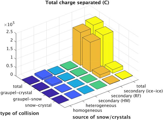
DECEMBER 2020                                              PHILLIPS ET AL.                                                                 3999

 Multiple Environmental Influences on the Lightning of Cold-Based Continental Cumulonimbus
                    Clouds. Part I: Description and Validation of Model

             VAUGHAN T. J. PHILLIPS,a MARCO FORMENTON,a VIJAY P. KANAWADE,a,h LINUS R. KARLSSON,a
           SACHIN PATADE,a JIMING SUN,b CHRISTELLE BARTHE,c JEAN-PIERRE PINTY,d ANDREW G. DETWILER,e
                                     WEITAO LYU,f AND SARAH A. TESSENDORFg
      a
        Department of Physical Geography, University of Lund, Lund, Sweden; b Institute of Atmospheric Physics, Chinese Academy of
      Sciences, Beijing, China; c Laboratoire de l’Atmosphère et des Cyclones, UMR 8105 CNRS/Météo-France/Université de La Réunion,
      Saint Denis, Réunion, France; d Laboratoire d’Aérologie, Université Paul Sabatier and CNRS, Toulouse, France; e Department of
        Physics, South Dakota School of Mines and Technology, Rapid City, South Dakota; f State Key Laboratory of Severe Weather,
        Chinese Academy of Meteorological Sciences, Beijing, China; g National Center for Atmospheric Research, Boulder, Colorado

                                       (Manuscript received 1 August 2019, in final form 5 June 2020)

         ABSTRACT: In this two-part paper, influences from environmental factors on lightning in a convective storm are assessed
         with a model. In Part I, an electrical component is described and applied in the Aerosol–Cloud model (AC). AC treats
         many types of secondary (e.g., breakup in ice–ice collisions, raindrop-freezing fragmentation, rime splintering) and pri-
         mary (heterogeneous, homogeneous freezing) ice initiation. AC represents lightning flashes with a statistical treatment
         of branching from a fractal law constrained by video imagery.
            The storm simulated is from the Severe Thunderstorm Electrification and Precipitation Study (STEPS; 19/20 June 2000).
         The simulation was validated microphysically [e.g., ice/droplet concentrations and mean sizes, liquid water content (LWC),
         reflectivity, surface precipitation] and dynamically (e.g., ascent) in our 2017 paper. Predicted ice concentrations (;10 L21)
         agreed—to within a factor of about 2—with aircraft data at flight levels (2108 to 2158C). Here, electrical statistics of the
         same simulation are compared with observations. Flash rates (to within a factor of 2), triggering altitudes and polarity of
         flashes, and electric fields, all agree with the coincident STEPS observations.
            The ‘‘normal’’ tripole of charge structure observed during an electrical balloon sounding is reproduced by AC. It is related
         to reversal of polarity of noninductive charging in ice–ice collisions seen in laboratory experiments when temperature or
         LWC are varied. Positively charged graupel and negatively charged snow at most midlevels, charged away from the fastest
         updrafts, is predicted to cause the normal tripole. Total charge separated in the simulated storm is dominated by collisions
         involving secondary ice from fragmentation in graupel–snow collisions.
         KEYWORDS: Atmospheric electricity; CAPE; Cloud microphysics; Freezing precipitation; Ice crystals; Ice particles

1. Introduction                                                           involving ice somehow, some modern explanations did not in-
    The first known books about weather phenomena were by                 volve ice (causes 1 and 2) and have been discounted.
Aristotle and his student, Theophrastus, in Ancient Greece                   With emergence of cloud physics, it has become apparent
around 300 BC (Brunschon and Sider 2007). In Meteorology,                 that no physical process occurs in isolation in clouds. Lightning
Theophrastus listed possible causes of lightning (Fortenbaugh             is no exception. Clouds consist of a myriad of interconnected
and Gutas 1992). A connection between ice in clouds and                   physical processes, including electrical processes. The charge
lightning was hypothesized. In modern times, lightning was un-            separation that causes lightning is known to be predominantly
derstood as an electrical process. In the twentieth century, var-         due to (noninductive) rebounding ice–ice collisions involving
ious causes were proposed for charge separation in clouds                 rimed ice precipitation in the presence of supercooled liquid
[literature reviewed by Pruppacher and Klett (1997, hereafter             (Reynolds et al. 1957; Takahashi 1978, 1984; Latham 1981;
PK97)]: 1) diffusion of ions onto inductively polarized drops,            Jayaratne et al. 1983; Baker et al. 1987; Helsdon and Farley
2) convection of space charge from the environment, 3) polarized          1987; Latham and Dye 1989; Kumar and Saunders 1989; H01;
drops colliding with ice and rebounding, 4) ice breakup, and              Helsdon et al. 2002, hereafter H02; Mansell et al. 2002, 2005,
5) ‘‘noninductive’’ charge separation in rebounding ice–ice               2010, hereafter M02, M05, M10, respectively). Sedimentation
collisions. Only cause 5 explained observed time scales                   of heavier particles leaves a net charge aloft. Overall charge
of electrification (Helsdon et al. 2001, hereafter H01). Whereas          separated depends on concentrations of ice, while charge
an explanation of lightning by Theophrastus assumed collisions            separated per collision is governed by temperature (T), liquid
                                                                          water content (LWC), and particle sizes. Essentially, lightning
                                                                          is caused by microphysical interactions.
  h
    Current affiliation: Centre for Earth, Ocean and Atmospheric             Microphysical processes in clouds are controlled by en-
Sciences, University of Hyderabad, Hyderabad, India.                      vironmental factors, such as aerosol conditions, instability,
                                                                          shear, and humidity. Aerosol conditions govern numbers
  Corresponding author: Vaughan T. J. Phillips, vaughan.phillips@         and sizes of cloud particles (Rosenfeld and Lensky 1998;
nateko.lu.se                                                              Phillips et al. 2001, 2002, 2005; Khain et al. 2004, 2005, 2008;

DOI: 10.1175/JAS-D-19-0200.1
 2020 American Meteorological Society. For information regarding reuse of this content and general copyright information, consult the AMS Copyright
Policy (www.ametsoc.org/PUBSReuseLicenses).
                                                                                                      Unauthenticated | Downloaded 12/03/21 07:32 AM UTC
4000                               JOURNAL OF THE ATMOSPHERIC SCIENCES                                                          VOLUME 77

van den Heever et al. 2006; Kudzotsa et al. 2016). There are            observed by aircraft in that case—including ice concentration and
two aerosol-sensitive mechanisms of precipitation:                      LWC. Here the simulation is repeated including the electrical
                                                                        component.
d   Cloud droplets coalesce to form rain depending on solute
                                                                           STEPS occurred in the U.S. central Great Plains (CGP),
    aerosol concentrations, if cloud base is warm (‘‘warm rain
                                                                        combining electrical (e.g., by balloon), radar, and micro-
    process’’). Supercooled rain in warm-based clouds (Koenig
                                                                        physical observations with an armored aircraft sampling fast
    1963; Hallett et al. 1978; Blyth and Latham 1993; Blyth et al.
                                                                        thunderstorm updrafts (Lang et al. 2004). A Lightning Mapping
    1997; Williams et al. 1999) can freeze (Bringi et al. 1997) into
                                                                        Array (LMA) was deployed (Rison et al. 1999; Krehbiel et al.
    ice precipitation (Phillips et al. 2001, 2002, 2005).
                                                                        2000). The storm case (19/20 June) was selected as 2CGs and
d   For cold (e.g., #08C) cloud bases, the ‘‘ice-crystal process’’
                                                                        normal electrical structure were observed. In CGP, most storms
    involves growth of crystals (e.g., from solid aerosols) to
                                                                        chiefly produce negative (2CG) lightning (Orville and Huffines
    ‘‘snow’’ (large crystals or aggregates) that may rime into
                                                                        2001; Boccippio et al. 2001; Fleenor et al. 2009), which is shown
    graupel.
                                                                        to be due to normal polarity charge structure (Tessendorf
Relative humidity (RH) controls the temperature of cloud                et al. 2007).
base (Williams and Stanfill 2002; Khain et al. 2004; Williams              The aim of this two-part paper is to unravel some of the mys-
et al. 2005; Zeng et al. 2009).                                         teries about environmental influences on lightning. First in this
   The vertical structure of charge characterizes thunder-              Part I the model and STEPS simulation are explained and vali-
storms. Most typically, a storm is ‘‘normal’’ (Williams 1989)           dated with observations. In Phillips and Patade (2020, manuscript
with a tripole (lower positive charge beneath midlevel                  submitted to J. Atmos. Sci., hereafter Part II), the simulation will
negative charge with upper-level positive charge) or dipole             be analyzed with sensitivity tests to quantify the environment–
(Kuhlman et al. 2006), causing negative cloud-to-ground                 lightning linkage. Focus is given in Part II to reasons for why
flashes (2CGs; negative charge to ground). Rarer storms                 lightning is observed more frequently over land than ocean and to
with the opposite configuration are ‘‘inverted’’ (Marshall              how the environment controls the charge structure of storms.
et al. 1995), with negative charge at upper levels and
‘‘1CGs’’ (positive charge to ground). More intense con-                 2. Model description
vection can be inverted with mostly 1CGs and often large                  The description by Phillips et al. (2017b) applies here in
hail (Rust et al. 1981; Reap and MacGorman 1989; Wiens                  nonelectrical respects with only a few minor changes. Symbols
et al. 2005).                                                           used in this paper are summarized in appendix A.
   For our cloud model, representations of ice-microphysical
processes were developed (Phillips et al. 2013, 2014, 2015, 2017a,      a. AC model
2018). Sticking efficiency for ice–ice collisions was treated with an      AC represents clouds and aerosols with hybrid spectral
energy-based approach (Phillips et al. 2015). Breakup in ice–ice        bin/two-moment bulk microphysics, interactive radiation, and
collisions was treated for all microphysical species and predicted      semiprognostic aerosol schemes. Here AC is run as a cloud-
by to form most (95%–98%) of ice particles not from homoge-             resolving model (CRM) with horizontal and vertical grid spac-
neous freezing in a ‘‘cold-based’’ (cloud base of about 08C) me-        ings of 1 and 0.5 km, and a 3D mesoscale domain 80 km wide.
soscale multicellular storm (Phillips et al. 2017a,b). The storm        Mesoscale cloud systems are resolved. Microphysical species
was observed on 19/20 June 2000 in the Severe Thunderstorm              are cloud liquid, cloud ice (or ‘‘crystals’’), rain, graupel/hail and
Electrification and Precipitation Study (STEPS) (Lang et al.            snow. Seven aerosol species govern primary initiation of hy-
2004). The ice-crystal process prevailed in the overall production      drometeors, with heterogeneous and homogeneous nucleation
of precipitation.                                                       of ice. Three types of fragmentation are treated to form secondary
   In the simulated STEPS storm, inclusion of breakup in ice–           ice: breakup in ice–ice collisions (Phillips et al. 2017a,b), Hallett
ice collisions increased the average concentration of ice by            and Mossop (1974, hereafter HM) rime splintering (cloud
between one and two orders of magnitude from 08 to 2308C                droplets . 24 mm) and fragmentation of freezing rain/drizzle
(Phillips et al. 2017b, their Figs. 5d and 8). Only by including        (Phillips et al. 2018). More details are in appendix B.
this breakup were aircraft observations of filtered (.0.2 mm)
ice concentration and LWC predicted realistically. Collisions           b. Electrical component
of snow (.0.3 mm) with denser graupel/hail initiated most of               The degree of complexity of the lightning scheme resembles
the secondary fragments. Surface precipitation was modified             that of Barthe et al. (2005) and is intermediate between those
by breakup with smaller crystals and less LWC.                          of H02 and M02/M05. This compromise minimizes computa-
   In this two-part paper, to compare influences on lightning           tional expense and facilitates understanding by excluding
from various environmental factors, an electrical component             nonessential processes.
is first developed and assessed for our Aerosol–Cloud model
(AC). AC represents all empirically quantified mechanisms                 1) CHARGE AND ITS SEPARATION IN ICE–ICE
for initiation of drops and crystals in terms of dependencies                 COLLISIONS
on aerosol conditions. This electrical assessment is performed with        Charge on hydrometeors is represented with a ‘‘space
the same cold-based cloud case from STEPS simulated and vali-           charge mixing ratio,’’ rq,x, for each xth microphysical species. It
dated by Phillips et al. (2017b) against coincident observations. AC    is a ‘‘bulk’’ quantity (i.e., for all sizes) transferred between
reproduced the many nonelectrical cloud-microphysical statistics        species by microphysical conversions. Charge density in air due

                                                                                                Unauthenticated | Downloaded 12/03/21 07:32 AM UTC
DECEMBER 2020                                            PHILLIPS ET AL.                                                               4001

to ions/charged aerosols, rq,a , is assumed to have a source            otherwise. Charge separated per ice–ice collision, whether or
from evaporation of charged drops (from prior melting of                not rebounding, was extrapolated with a dimensionless pa-
charged ice) or sublimation of charged ice, but not from                rameter, a:
diffusional growth (e.g., Barthe et al. 2005). In the labora-
tory, during evaporation of any charged drop, only when it                     dQ 5 aMIN[QTaka (T, LWC*), QTaka (T, LWC)]
has completely disappeared is charge seen to transfer to
                                                                                     3 [(1 2 j) 1 jc] " 08 . T . 2308C ,                (1)
the air, and the same would be expected for ice. Hence in
AC, during any evaporation/sublimation of particle size                 where QTaka is the function plotted by Takahashi (1978,
distributions (PSDs), it is assumed that there are always               Fig. 8 therein), fitting his own data. Here j(T . –208C) 5 0
some hydrometeors small enough to disappear totally. No                 and j(T , –258C) 5 1, while c(LWC , 0.01 g m23) 5 0 and
recombination of charge in air is represented, since nega-              c(LWC . 0.05 g m23) 5 1. Both are linearly interpolated
tive or positive ions/charged aerosols are not separately               in between. Here the actual LWC in Takahashi’s original
resolved. No sinks of ions on cloud particles are treated.              formula has been replaced with LWC* in Eq. (1) when doing
   For ice–ice collisions, the emulated bin scheme involves tem-        so decreases QTaka. At T . 2208C, LWC* 5 LWC. Takahashi
porary grids of bins discretizing size distributions (section 2a) and   counted all collisions irrespective of whether they rebound, so
schemes for sticking (Phillips et al. 2015) and collision               Eq. (1) applies to all collisions too.
(Khain et al. 2001; Pinsky et al. 2001) efficiencies. ‘‘Bulk’’             For T , 2248C and LWC , 0.2 g m23, practically no ob-
charge separated in collisions is from summing contribu-                servations were made by Takahashi (1978), who extrapolated
tions over permutations of bin pairs. Only rq,x is then al-             QTaka into this unobserved region assuming positive charging
tered. Charge per particle, q(D) 5 bDg, is assumed in any               of the rimer. Negative charging was observed for LWC $
species (Beard and Ochs 1986; MacGorman and Rust 1998;                  0.2 g m23 at T , 2248C. By videosonde in cold-based (08C)
Barthe et al. 2005, 2012); D is particle diameter, g is pre-            clouds (tops near 2258C), graupel was seen to be charged
scribed with a fixed value, and b is evaluated numerically              negatively below and positively above the 2118C level
from rq,x. The bulk charge is distributed among all particles           (Takahashi et al. 2017). Peak LWC was 0.4 g m23 so this
of a temporary grid of bins, so that larger particles have              reversal (2118C) was warmer than for Takahashi’s (1978)
more charge per particle.                                               lab data (see also Pereyra et al. 2008).
   There are two main groups of schemes for noninductive                   Consequently, at weak LWCs if T , 2208C the unob-
charge separation from laboratory studies:                              served charging of the rimer is assumed to be negative with
1) Takahashi (1978, 1984);                                              values from the adjacent observed region at 0.2–0.5 g m23
2) Jayaratne et al. (1983), Keith and Saunders (1989),                  (section 5b):
   Saunders et al. (1991), Brooks et al. (1997), and Saunders                       8
                                                                                    >
   and Peck (1998).
                                                                                23
                                                                        LWC [g m ] 5 " 0:01 , LWC , 0:5 g m23 and T , 2208C .
                                                                           *
At weak LWCs (e.g., 0.1 g m23) Takahashi observed positive                          >
                                                                                    >
                                                                                    :
charging of the rimer at most temperatures while Saunders                            LWC, otherwise
et al. show negative charging. Reasons for such differences are                                                                         (2)
uncertain. Experiments differ in design between the two
groups, 1 and 2 (e.g., Saunders et al. 2006).                           Equation (2) improves a simulation, not shown here, of an
   We opted for group 1. This allowed 2CGs and a ‘‘normal               inverted storm with 1CGs observed by Wiens et al. (2005).
tripole’’ structure to be simulated, as observed in the case            With more prolific negative charging of the rimer at weaker
(sections 1 and 4). A faster impact speed in group 1 (8 m s21)          LWCs, the central positive charge of the inverted storm from
approaches convective updraft speeds (10–15 m s21) observed             fallout of graupel/hail is strengthened, favoring 1CGs.
here (Tessendorf et al. 2007; Phillips et al. 2017b), similar to fall      Takahashi (1984) proposed that charge separated is pro-
speeds of graupel/hail balanced in them. Real flash rates in-           portional to the difference in fall speeds and surface area of the
crease with updraft speed (Williams et al. 1985; Zipser and             crystal. Thus, diameter (Di) and fall speeds govern a:
Lutz 1994; Boccippio et al. 2001). Hail below normal thun-
                                                                                               "             2                  #
derstorms is seen to be mostly positively charged (Kuettner                                            Di,*        jVp – Vi j
1950; Rust and Moore 1974; Magono 1977; Wahlin 1986),                                a 5 MIN 3J                              , 100 ,    (3)
                                                                                                       D0              8
consistent with positive charging of graupel/hail simulated
by AC (section 5b). Laboratory observations by Pereyra                            Di,* 5 MIN(Di , 0:3Dp ).                              (4)
et al. (2000), Berdeklis and List (2001) and Takahashi and
Miyawaki (2002) at weak LWCs agreed better with group 1                 Unrimed (cloud ice/snow) and rimed (graupel/hail or riming
than group 2.                                                           snow) particles are denoted by subscripts ‘‘i’’ and ‘‘p.’’ Also
   Takahashi (1978) observed the average charge, QTaka, sep-            D0 5 100 mm. The contact area cannot be wider than some a
arated per collision between a rimed rod (3 mm, representing            fraction of the rimer, hence Di,* . Inspection of laboratory data
graupel) and crystals (100 mm) from 08 to 2308C. Charging was           by Takahashi (1987, his Fig. A3) implies it is 0.3.
seen to depend on T (8C) and LWC, with positive charging of                As Takahashi (1978) observed collisions of only cloud-ice
the rimer for T . 2108C but only for low or very high LWCs              crystals (0.1 mm) with a rimer, our inclusion of a new factor, J,

                                                                                               Unauthenticated | Downloaded 12/03/21 07:32 AM UTC
4002                              JOURNAL OF THE ATMOSPHERIC SCIENCES                                                            VOLUME 77

in Eq. (3) treats other types of collision too. For collisions        a 3D cubic grid of 0.5-km resolution) is much wider (by
of graupel with cloud-ice crystals, J 5 1. For graupel–snow           50%) and higher than the dynamics domain for open lat-
collisions, the charge transferred is assumed proportional            eral (eastern and western) and upper boundaries, following
to the bulk density of snow, which determines the total area          M05. Northern and southern lateral boundaries coincide and
of many microscopic solid contacts, not counting air spaces,          are periodic for both domains. The electric field, E 5 2=f, is
during impact. Indeed, the charge transferred by collision            calculated on the potential domain with potential, f, from
of a 1-mm frost particle with a large rimed target (Takahashi         solving the Poisson equation for net space charge density,
1987, his Fig. A3) is seen to be lower by a factor of 25 than         rq (Adams 1989). For the potential domain, horizontal compo-
expected by areal extrapolation from 0.1 mm (Takahashi                nents of electric field are zero on lateral open boundaries (M05,
1978). This factor approximates the ratio of bulk densities           M10) far from the dynamics domain, while upper and lower
between a 1-mm snow particle and a 0.1-mm crystal in AC               boundaries are prescribed with the background potential and
(800:40) (see also Heymsfield et al. 2002, their Fig. B1).            zero volts, respectively. In clear-sky conditions the fair-weather
Hence we assign J 5 rs /800 for graupel–snow collisions               electric field is reproduced (e.g., about 250 and 25 V m21 at
and J 5 rs/600 for snow–crystal collisions. Here rs is the bulk       1.6 and 10 km MSL; e.g., PK97). The upper boundary (30 km
density of snow (kg m23) while 800 and 600 kg m23 are the es-         above ground) is so high that fixing its potential has little in-
timated bulk densities of cloud-ice crystals (0.1 mm) and rime        fluence on the storm (cloud tops about 14 km above ground).
density of the target (Williams and Zhang 1996) respectively, in         Only after each flash and its partial neutralization of charge
the laboratory experiment of Takahashi (1978).                        is f evaluated. This is less expensive than frequent updates of
   At T , 2308C, then dQ is multiplied by fTaka(T), which is          electric field in more explicit models (e.g., M02; Fierro et al.
zero when colder than 2408C and unity at 2308C, being in-             2006). Though electric fields may influence coagulation (re-
terpolated in between (fTaka 5 1 2 [(T 1 30)/10]2 for 2308 .          viewed by PK97), such effects are neglected here.
T . 2408C). Also, QTaka(T , –308C, LWC) 5 QTaka(–308C,
LWC). From Eq. (1), 6dQ is added to rq,x per collision among            3) LIGHTNING
different species unless the sticking efficiency is unity (Phillips      Lightning is simulated partly following MacGorman et al.
et al. 2015). When the entire rimer is covered in liquid (Phillips    (2001) and Barthe et al. (2005) with some modifications. The
et al. 2014) or when LWC , 0.01 g m23, then dQ 5 0 is                 discharge is triggered where E 5 jEj reaches a threshold
assumed.                                                              (Marshall et al. 1995; Riousset et al. 2007; Krehbiel et al.
   Equations (2) and (4) are unique here. The original factor of      2008) in V m21 of
(Di/D0)2 for a in (3) must have somehow represented the ratio
of areas of contact between the actual and observed (D0 5                                    Einit 5 1:8 3 105 ra (z).                    (5)
100 mm) collisions. Charge separation is an interfacial phe-
nomenon. Takahashi (1984) thresholded a to be , 10 since              The plasma channel is modeled as two leaders with opposite
Marshall et al. (1978) attributed saturation of charging to a         polarities of charge propagating from the trigger in opposite
limitation on contact area. We relax the threshold to 100 as it       directions. The positive and negative leaders propagate toward
was not directly observed and a similar limitation is present         negative and positive ambient charge, respectively, if preflash
in (4). The physically plausible dependency on contact area,          fields exceed a fraction, fprop 5 5%, of Einit; Winn et al. (1978)
and similarity of morphologies of snow and crystals on the            observed 15 kV m21 fields below a thunderstorm. Propagation
microscopic scale, suggests the validity of extrapolating             stops if the channel doubles back. Each leader is traced exactly
beyond laboratory conditions to any crystal size and per-             parallel or antiparallel to the preflash electric field vector ir-
haps to graupel–snow collisions. Yet charging in graupel–snow         respective of gridpoint locations. The same lateral boundary
collisions was never studied by Takahashi (1978). Conceivably, a      conditions are applied to leaders and their branches as for
slightly different dependence of charging on contact area for         other predicted quantities. Any leader crossing a periodic
snow than crystals may exist in reality (Takahashi 1987). Two         boundary simply reenters on the other side.
key morphological differences between ‘‘cloud-ice’’ crystals             A 2CG (1CG) occurs if a leader goes below 1.5 km (3 km)
(,0.3 mm) and snow (.0.3 mm in AC) exist: bulk density                above ground. This threshold is from observations by a light-
drastically decreases for snow aggregates as size increases and       ning positioning system at Guangzhou (Lyu et al. 2014, 2016;
the presence of multiple monomers per snowflake boosts the            Fan et al. 2018) and in STEPS (Wiens et al. 2005). Also the
sticking efficiency (Phillips et al. 2015).                           potential of the trigger point, f0, must satisfy f0 3 rch $ 0
   In summary, Eqs. (1)–(4) are applied for charging in               where rch is charge density in the leader approaching ground
collisions between graupel/hail and crystals, graupel/hail            (positive for 1CGs, negative for 2CGs) and jf0j . 20 M V (Tan
and snow, and riming snow and crystals. Only charging in              et al. 2014, their Fig. 3). If both criteria are met, the leader is sent
graupel–crystal collisions was observed in the laboratory by          vertically to ground.
Takahashi, however.                                                      Branches are treated statistically, without tracing channels,
                                                                      when jrqj . rcrit 5 0.2 nC kg21 and ambient f is lower (higher)
  2) ELECTRIC FIELD                                                   than the positive (negative) leader’s f0. A grid box must satisfy
   AC uses two domains, a ‘‘dynamics domain’’ for prognostic          both conditions and be adjacent to one satisfying them so as
variables inside an extended finer ‘‘potential domain’’ for elec-     to be added to the branch cluster of a leader. The maximum
trical quantities. The potential domain (120 km 3 80 km 3 30 km;      number of branching grid boxes is (Barthe et al. 2005)

                                                                                               Unauthenticated | Downloaded 12/03/21 07:32 AM UTC
DECEMBER 2020                                                  PHILLIPS ET AL.                                                               4003

  FIG. 1. Schematic diagram of the flashes branching algorithm as
applied to a single flash. Two leaders propagate upward and
downward from the trigger point. The branching volume around
each leader is divided into many concentric hemispheric shells.
Each hemispheric shell depicted here has a certain number of
branches according to the number of its junction points.

                                          !x
                              r
                          N5                    .                    (6)
                             Lx

In this fractal law N is the number of junction points of
branches . 0.5 km in the sphere of radius r from the pre-
flash trigger point while L x is a length scale. Figure 1
conveys the geometry of fractal branching schematically.
The number of branch junction points of a polarity in the
jth hemispherical shell (dr) of radius r from the preflash
trigger point is
                              !x                         !x
             dr dN x 1                              x dL
       dN\ ’      5                  r   x21
                                               dL 5         jx21 ,   (7)
             2 dr 2 Lx                              2 Lx

             Ngrid (j) 5 k 3 dN\ ,                                   (8)

where Ngrid is the maximum number of grid boxes with branches
in the shell; k is the number of grid boxes (0.5 km) per junction
point of branches crossing them; dr 5 dL, where dL is the di-
agonal gridbox width and r 5 jdL. Equations (7) and (8) are
unique. Appendix C implies k ’ 7(Lx /dL). By cycling over all j
from the trigger, branched grid boxes of the leader are amassed.
   For constants in (7), three composite images of lightning
were taken from the Tall-Object Lightning Observatory in
Guangzhou (TOLOG) in China with a high-speed video
camera (Fig. 2). These were three downward 2CGs both in                       FIG. 2. Composite visible images of flashes to ground taken with a
and out of cloud, with upward leaders from tall structures.                high-speed video camera from Guangzhou City in southern China,
Junction points were counted for branches .0.3 km in pro-                  from (a) 22 Jul and (b) 7 and (c) 24 Sep 2012. The resolution is 3 and
jected length (plane normal to view), corresponding on aver-               4.7 m per pixel and the distance to the striking point is 2.1 and 3.3 km,
age to branches . 0.5 km in 3D. Trigger points aloft were                  for (a)/(b) and (c), respectively. These were all downward CGs, in-
                                                                           volving upward leaders from tall structures.

                                                                                                    Unauthenticated | Downloaded 12/03/21 07:32 AM UTC
4004 JOURNAL OF THE ATMOSPHERIC SCIENCES VOLUME 77
assumed near 2108C as typically observed there (Zheng et al.
2019). The mean for all three photos implies Lx ’ 1.4 6 0.2 km
(90% confidence interval, t statistics).
4) NEUTRALIZATION OF AMBIENT CHARGE BY
LIGHTNING
Ambient charge, on hydrometeors and air, is neutralized in
each grid box of the flash as follows. The charge in the flash is
rch 5 zjrq 2 rcritj where z 5 2rq/jrqj is the polarity of plasma
with opposite sign to the net ambient space charge density,
rq 5 rq,a 1 åx rq,x . Ambient space charge densities in air and in
each xth species, rq,a and rq,x, are incremented by drq,a 5
zMIN(jrchj, jrq,aj) and drq,x 5 zMIN(jrch 2 drq,aj, jrq,xjx x), while
x x is its fractional contribution to total hydrometeor surface area.
Neutralization is incomplete in nature (Williams et al. 1985), as
treated by rcrit. For ICs, drq,a and drq,x are normalized to
have a total charge of zero over the flash, before altering rq,a
and rq,x. The normalization is not done for CGs as net
charge in the flash after neutralization flows to ground.
3. Description of observed case and model setup
STEPS in summer 2000 observed convective storms by
aircraft, balloons, radar, ground-based measurements, and
satellite (Lang et al. 2004). The storm on 19/20 June had high
cold cloud bases near 08C (4.4 km MSL) at 3 km above
ground (1.3 km MSL). The case is representative of conti-
nental multicell storms in U.S. CGP (section 1) where cloud
bases are usually colder than further south. It was a multicell
system of convection 50–100 km wide.
The storm began over Colorado at about 2200 UTC (1600
local time) and moved almost eastward (about 708 from north).
Graupel (,0.5 cm) and snow were ubiquitous in aircraft obser-
vations. During flights, small hail (.0.5 cm) was detected,
especially on flanks of convective updrafts (Goehring 2005; FIG. 3. (a) The total flash rate in the simulated domain, predicted
Phillips et al. 2017b). Convective cells (reflectivities up to (closed circles) and observed (thin line) for the STEPS case
55 dBZ aloft) coexisted with a lightly precipitating stratiform (2345 UTC 19 Jun–0215 UTC 20 Jun 2000). Lightning data ob-
cloud deck (about 20 dBZ). served by LMA were computed on a moving grid that followed the
The multicellular storm is simulated in a 3D domain model domain (Phillips et al. 2017b). Also shown is (b) the cu-
(80 km 3 80 km 3 16 km), approximating it as a convective line mulative distribution of vertical velocity between 5 and 6.5 km
with cells initiated at x 5 30 km. Translation of the domain MSL in fast convective updrafts .5 m s21, comparing the predic-
tion (thick line) with observations by aircraft and Doppler radar
keeps them in it. The horizontal x axis points 708 from north.
(lines with symbols). Transient fluctuations of up to about 3 m s21
Phillips et al. (2017b) elaborate further.
arose from flight maneuvers, so the relative error in aircraft data of
ascent is assumed to be 630%.
4. Results from model validation
Regarding nonelectrical quantities, Phillips et al. (2017b,
their Figs. 5 and 6) showed agreement between the AC simulation statistics at flight levels of 6–7 km MSL. The flash rate is sim-
of the STEPS case (1145 UTC 19 June–0215 UTC 20 June 2000; ulated with errors mostly less than a factor of 2. Aircraft data of
section 3) and coincident observations by aircraft, satellite, and ascent are more accurate than the radar data and agree with the
ground-based instruments for many quantities. Vertical profiles of predicted ascent at all cumulative frequencies of vertical ve-
mean diameter and concentration of droplets, LWC, radar re- locity. Dual-Doppler ascent retrievals have wide biases (Dahl
flectivity, filtered ice concentration, and PSDs were among et al. 2019).
quantities predicted accurately. Predicted and observed concen- Figure 4 depicts numbers of all flashes. Most (.99%) are
trations of ice particles (.0.2 mm) identically averaged in con- IC, the rest (1%) 2CG. Model and observations agree,
vective updrafts were on the order of 10 L21 at flight levels. differing by about 10%. A few (4%) observed CGs were
Differences between prediction and observations were less apparently 1CG as predicted, though misclassification of
than the spread of observations. ICs as 1CGs is possible (Cummins et al. 1998; Leal et al.
With electrification represented, Fig. 3 compares predicted 2019). The IC/CG ratio of 102 is large (Lang et al. 2000;
and observed flash rates (Tessendorf et al. 2007) and ascent Williams 2001; Boccippio et al. 2001). A high cloud base
Unauthenticated | Downloaded 12/03/21 07:32 AM UTCDECEMBER 2020 PHILLIPS ET AL. 4005
FIG. 4. Observed and simulated (AC) total numbers of flashes
for the three types of lightning in the STEPS case (2345–
0215 UTC), namely, intracloud (IC; black), negative cloud-to-
ground (2CG; gray), and positive cloud-to-ground (1CG; white)
lightning. For observed flashes, only those in the 3D domain sim-
ulated (Phillips et al. 2017b, their Fig. 1a) are counted.
(3 km above ground) from a dry lower troposphere in-
hibited charged surface precipitation and hence CGs, for
reasons noted below.
Figure 5 shows 2CGs and estimated altitudes of trigger
points. Observations and predictions agree in timing and
frequency. Most 2CGs were initiated in convective cloud
near 6–7 km MSL (2108 to 2178C), in the lower half of the
central negatively charged region (5.5–9 km MSL) of the
large-scale tripole. Heights of triggering for all flashes are
predicted adequately, but with a peak 2 km too high FIG. 5. Negative cloud-to-ground flashes for the STEPS case
(2345–0215 UTC), observed (open symbols) and predicted by AC
(Fig. 5b). Observed and predicted ICs were mostly initiated
(closed symbols). (a) Their time evolution in terms of numbers of
at 6–9 MSL altitude (about 2108 to 2308C) with a peak near
2CGs every minute (black and blue lines). (b) The vertical profile
8 km MSL (about 2258C). They were predicted to arise of relative frequencies of their estimated trigger-point altitude.
often from intense charge of transient graupel/hail fall Also shown in (b) is the corresponding vertical profile for all
shafts in convective cells, at levels in the midst of the central flashes, the vast majority of which are IC. Finally, superimposed in
negative region of the large-scale tripole. A few flashes (a) is the time evolution of accumulated absolute magnitude of
(10%) were observed to trigger at 3–5 km MSL, especially charge at the ground (red lines) from precipitation (positive) and
ICs at 4.4–5 km MSL (08 to 248C; 0110 to 0200 UTC), levels CGs (negative).
where none are predicted (section 6).
Timing of 2CGs is explicable in terms of surface precipi-
tation (Fig. 5a). Predicted accumulation of charge in surface why arrival of surface precipitation in the second half of
precipitation from similarly charged graupel causes that of the simulation (Phillips et al. 2017b, their Fig. 5) coincides
opposite charge to ground from CGs (section 5b), as with all with 2CGs. Generally, onsets of CGs and surface precipitation
simulations in Part II (not shown), leading it by 10–20 mins, are observed to coincide to within a few mins (Gungle and
because removal of charge in precipitation creates the total Krider 2006) with CG number controlled by rainfall volume
storm charge aloft. In normal (inverted) storms, AC predicts (Battan 1965; Kinzer 1974; Piepgrass et al. 1982). Here, to
net transfer of positive (negative) charge to the surface in summarize, positive charge of surface precipitation causes
precipitation and then 2CGs (1CGs) as a lagged response in negative average charge on the simulated normal storm
all simulations. As most 2CGs or 1CGs originate from mid- and 2CGs as a response. Corona discharge may complicate
levels and conduct negative or positive charge toward the this picture (section 6). Equally, charged precipitation
higher or lower potential of the ground (always zero volts), shafts below cloud promote propagation of CGs downward.
respectively, they respond to the total of all net charge and Number density of LMA sources (VHF) was observed in
average potential of the entire convective core caused by STEPS. They have no polarity, but the negative end of a flash
fallout of oppositely charged precipitation to ground. This is produces more sources (e.g., Dwyer et al. 2004, 2005) than the
Unauthenticated | Downloaded 12/03/21 07:32 AM UTC4006 JOURNAL OF THE ATMOSPHERIC SCIENCES VOLUME 77
other end, so polarity of ambient volume can be inferred. For
comparison, this source density is diagnosed from AC output
by assuming proportionality with charge neutralized in each
grid box, a novel method. The constant of proportionality gives
observed numbers (;103) of sources per flash for storms gen-
erally (Wiens et al. 2005). The constant (200 or 50 nC21) is 4
times higher for ‘‘positive LMA’’ sources (negative breakdown
through ambient positive charge) than negative sources (vice
versa), as seen in storms by Wiens et al. (2005), Rison et al.
(1999) and the case here.
Figure 6 shows agreement between predicted and observed
profiles of total, positive and negative LMA sources for cloudy
levels (4–13 km MSL). There are deep broad maxima for all
and positive sources near 25 and 23 dB, respectively, over 5–
10 km MSL (about 258 to 2408C) and a narrower peak of
negative sources of about 20 dB. Predicted negative LMA
sources are about 1 km too high, consistent with ICs being
triggered at levels too high also.
Figure 7 shows horizontal distance of predicted trigger
points from maximum ascent (13 6 4 m s21) in the nearest
convective core. Most (97%) are in the core. About 3% are
in stratiform/cirriform cloud, being triggered ‘‘remotely,’’
10–20 km from the core’s maximum ascent, with a few
(0.02%) 18–20 km away. A compass plot shows simulated
trigger points in the horizontal plane relative to the nearest
core (Fig. 7b). Favored locations of remote trigger points
(.10 km) are between adjacent cells where electric fields
superpose. Triggering here slightly prefers sides of any cell
that are upshear and to the left of the system’s propagation
direction, because the environmental vertical shear is not
unidirectional.
Most charging of graupel occurs in convective ascent
(section 5b). Yet broad continua of sizes and fall speeds of
graupel in any cloudy volume create vertical charge struc-
ture in the layer cloud from outflow, causing a continuous
distribution of horizontal distances of triggering from the
core (by up to 20 km away here). The prediction (Fig. 7) ac-
cords with observations of most lightning being triggered in
cores and with a few flashes triggered tens of kilometers away
(Proctor 1991; Wiens et al. 2005; Dye and Willett 2007; Weiss
et al. 2012; Kuhlman et al. 2009). Supercooled cloud liquid
must be present for any charge separation to occur in AC.
In the STEPS case, electrical properties of the storm were
measured by balloon. Figure 8 shows the balloon trajectory,
initially 20 km downshear of convection (,50 dBZ) in weak
reflectivity (about 0 dBZ). Struck by lightning at 9 km MSL, all
other flashes around it were triggered at least 5 km away
(Fig. 8). The balloon rose through layer cloud toward the
FIG. 6. The density of (a) all LMA sources expressed in decibels
(dB; 10log10[number of average sources per min per volume ele-
ment (min21)]) for the AC simulation (2345–0215 UTC) (thick full
line) and STEPS observations from the region (80 km 3 80 km)
simulated (dashed line). In both observations and simulation, the positive charge) and (c) negative (vice versa) LMA sources are
3D domain is divided into volume elements 0.5 km deep and compared similarly. Errors of the prediction arise from choice of
10 km wide in one horizontal direction, spanning the domain in average value of LMA sources per flash (about 1000), which may
the other, with averaging over all elements at each level (Wiens vary by about half an order of magnitude (e.g., Wiens et al. 2005).
et al. 2005). The source profiles in dB for every minute are then The error shown for the observed profile is the standard devia-
averaged over the simulated period. Corresponding contribu- tion for the variability over time. For simplicity, the observations
tions from (b) positive (negative breakdown through ambient were analyzed over a fixed domain of the same size as the model.
Unauthenticated | Downloaded 12/03/21 07:32 AM UTCDECEMBER 2020 PHILLIPS ET AL. 4007
component of E. Figure 9b compares it with AC’s ensemble.
A normal tripolar charge structure (e.g., Williams 1989) is
predicted and observed:
d weak positive charge below the 2108C (6 km MSL) level;
d strong negative charge at 6.5–8 km MSL (about 2158 to 2258C);
d moderate positive charge at 8–10 km MSL (about 2258
to 2388C) aloft.
Normal tripoles are associated with predominance of 2CGs
among strikes to ground, as in the simulation. Most2CGs were
triggered at lower levels of this central negative region, where
negatively charged snow remains as graupel/hail falls out. The
normal tripole is here predicted for reasons (central negative
charge due to snow/crystals, rather than graupel) differing
from the traditional explanation of normal tripoles (Williams
1989) (section 5a).
Figure 10 compares predicted charge to ground in 2CGs
with that inferred from peak currents (Rakov and Uman 2003;
Schoene et al. 2010) observed in STEPS. They agree in terms of
both the median charge per flash and the statistical distribution
among all flashes to ground.
5. Results for other electrical quantities of STEPS case
a. Spatial distribution of predicted charge and electric field
Figure 11 shows space charge density averaged over the
domain. Features seen in the balloon sounding (Fig. 9) are
evident. The most intense charges are on graupel (positive)
and snow (negative). The net charge in the storm is from
differential sedimentation of graupel versus snow/crystals.
Most charge on graupel is from rebounding collisions with
(cloud-ice) crystals, the process observed by Takahashi (1978)
FIG. 7. From the AC simulation are shown (a) relative frequency
(section 2b). Once charged, many crystals grow to become
of the horizontal distance of the trigger points from the center of
charged snow. Fluctuations of LWC below average are the
the nearest convective core for all flashes of the STEPS case (2345–
0215 UTC) and (b) their relative positions compared to this com- cause of graupel mostly charging positively (section 5b), as
posite core in terms of flash density (logarithm of number per km2) noted below.
in the horizontal plane. The vast majority are IC. In (b), the origin The normal tripole in Fig. 11 is explicable as follows. First, at
of the compass plot is the axis of the strong convective updraft midlevels below 10 km MSL (about 2388C), the averaging
nearest to each trigger and the blue arrow delineates the direction includes regions of negative and positive charge on graupel in
of storm propagation. Angles in (b) are directions defined clock- extreme (rich LWC) and moderate/weak (low LWC) convec-
wise from north while distances are in km. tive ascent, respectively. Weaker ascent is wider and prevails,
so graupel charges mostly positively. Above 8–9 km MSL
downshear anvil of approaching cells, missing them (Goehring (near 2308C) the polarity of both oppositely charged ice spe-
2005, Fig. 26 therein). cies dominating charging (graupel and cloud-ice crystals) in
Figure 9 compares quantities measured by balloon and Fig. 11 reverses, as in the laboratory data of charging
simulated for an ensemble (30) of virtual balloon trajectories. (Takahashi 1978, his Fig. 8). In the laboratory the rimer was
The AC simulation is idealized and cannot reproduce positions seen to charge negatively at LWCs . 0.1 g m23 if T , 2308C,
of real clouds. From AC output, each trajectory was traced, but always positively if T . 2108C (section 5b). Graupel in
ascending 7 m s21 faster than the evolving wind to match ob- the fastest ascent (LWC ; 1 g m23) becomes negatively
served altitudes. Trajectories were initiated randomly from a charged when T , 2158C, being upwelled into cirriform
square (10 km) about 10 km east of a cell with a similar re- outflow aloft. Conversely, graupel in moderate/weak con-
flectivity to that near the real balloon. The predicted mean vective ascent charges positively and likely remains at lower
electric field (Fig. 9a) agrees with the observations. The max- levels, detraining into stratiform cloud.
imum measured was 30 kV m21 (8 km MSL), much weaker than Net charge in narrow graupel/hail shafts (6–8 km MSL;
the breakdown threshold (90 kV m21). The balloon sampled 2108 to 2258C) is predicted to be mostly positive. This
large-scale conditions ahead of the convective line. agrees with LMA observations of net charge being positive
Total space charge density, rq , is from the balloon at midlevels (6–8 km MSL) in a graupel/hail shaft (45 dBZ)
sounding using dE z/dz ’ rq/, where E z is the vertical next to an updraft (.5 m s21) from Tessendorf et al. (2007,
Unauthenticated | Downloaded 12/03/21 07:32 AM UTC4008 JOURNAL OF THE ATMOSPHERIC SCIENCES VOLUME 77
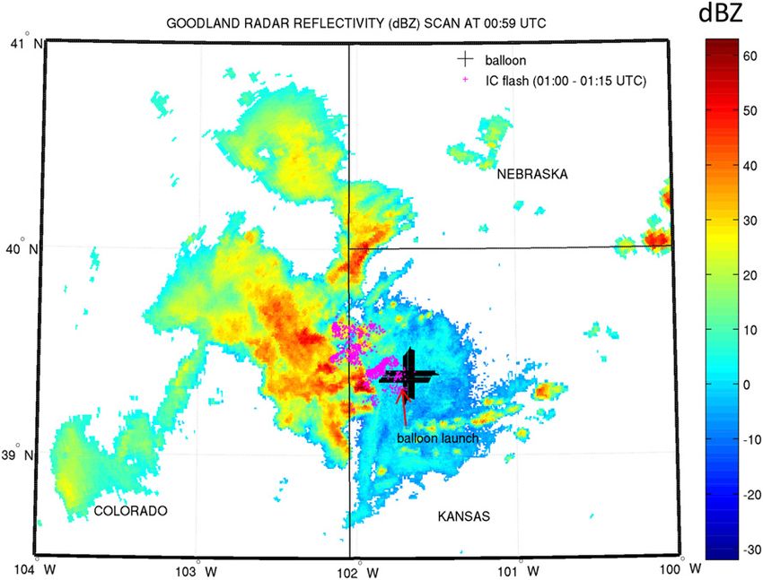
FIG. 8. Plan view of balloon trajectory (large black plus symbols) superimposed on a 0.488
elevation angle scan of equivalent reflectivity factor (dBZ) near the ground from the Goodland
radar at the moment of release (0059 UTC 20 Jun 2000). The balloon is almost 20 km to the east of
a reflectivity maximum of about 40 dBZ when launched and then drifts several kilometers
northeastward. Also shown are the IC flash trigger points (magenta tiny plus symbols) during
ascent of the balloon until it was struck by lightning at 9 km MSL altitude. The balloon was
launched by the National Severe Storms Laboratory (NSSL) from Goodland airport.
their Figs. 12c,d, their x 5 268 km) in this STEPS case at while cirriform and stratiform cloud is ice-only (Figs. 13a,b)
0019 UTC. In stratiform outflow (30–40 dBZ) from this due to weakness of ascent (Korolev 2007). Both charging and
updraft (0019 UTC), observed LMA sources are negative at graupel production (Figs. 12a,d and 13b,e,f) coincide in the
midlevels. Positivity of graupel/hail shafts is observed to cell. Graupel forms near updraft edges from riming of snow
coexist with average negativity on the large scale (.5 km), (Figs. 13d,e). Collisions between graupel and secondary
as in the simulation. cloud-ice crystals cause the charging.
In Fig. 11, at upper levels predicted net charge (positive A shaft of positively charged graupel falls from the
above 9 km MSL) is caused by cloud-ice crystals, which are downshear (eastern) side of the cell, leaving negatively
spread by their slow fall speeds coupled with large storm- charged snow/cloud ice aloft (Figs. 12b–d). Near 10 km MSL
relative flow over wide areas. Positivity of cloud ice and there is a widespread upper-level layer of positively charged
negativity of graupel are due to charge reversal in the labo- snow/cloud ice. Deep positive charge on graupel typifies the
ratory data, as noted above. At lower levels (5 km MSL), Takahashi charging scheme: in extreme ascent (.15 m s21)
weak positive net charge is from positively charged graupel supercooled liquid is sufficient (e.g., 1 g m23) for graupel
falling out. to charge negatively. Slightly negatively charged graupel
Comparing Figs. 5, 6, and 11 reveals that 2CGs, simu- (Fig. 12d) extends downshear from the cell near 10 km MSL,
lated and observed, originate from intense electric fields capping the positively charged graupel shaft below. Offline
between the strong central negative and low-level positive tracing of back trajectories of positively (z 5 6.5 km MSL,
centers of the large-scale tripole. ICs originate from most x 5 32 km) and negatively (z 5 8.5 km MSL, x 5 27.5 km)
subzero levels, but especially in the upper half (2208 charged graupel confirm
to 2308C) of the central negative region of the large-scale
d negatively charged graupel is from ascent .15 m s 21
tripole. ICs are often triggered near transient narrow shafts
(LWC . 1 g m 23 , 2108 to 2308C) and
of intensely charged graupel/hail (see snapshots below).
d positively charged graupel originates from weaker as-
Figures 12 and 13 show snapshots of electrical and mi-
cent (e.g., , 3 m s21) with LWC , 0.3 g m23 at warmer
crophysical quantities in vertical sections where lightning
levels (.2128C).
was triggered in a cell at 0055 UTC. Peak updraft speed is
15 m s21 with LWC , 2 g m23. Supercooled liquid is confined In much of the narrow shaft, the net space charge has the same
to the convective updraft (5 km wide) below the 2208C level, sign as the charge on graupel/hail (Figs. 12a,b). Three ICs in
Unauthenticated | Downloaded 12/03/21 07:32 AM UTCDECEMBER 2020 PHILLIPS ET AL. 4009
FIG. 9. (a) The vertical component of electric field (Ez) both
observed (black open symbols) and predicted by AC (red closed FIG. 10. Observed (‘‘NLDN’’) and predicted (‘‘AC’’) amounts of
symbols). Measurements were from an electric field meter on the negative charge in any flash to ground among all 2CGs in the
balloon plotted in Fig. 8. The full line of the model is the mean of an simulated region of STEPS. The logarithm of the absolute mag-
ensemble of many possible simulated trajectories of the balloon. nitude of the charge transferred to ground is shown. The 2CG
Positive values indicate an upward electric field. (b) A vertical flashes are the same set shown in Fig. 4. Charge was inferred from
profile of the inferred net charge density from the same balloon NLDN observations of peak current by assuming proportionality
observations (black open symbols) compared with the average for to the square of the peak current in view of empirical relations for
the ensemble of simulated trajectories (red closed symbols). Both rocket-induced artificial lightning by Schoene et al. (2010, their
model and observations depict the large-scale normal tripole of Fig. 4). The constant of proportionality was constrained by general
charge structure. Errors plotted in (a) and (b) are standard devia- known characteristics of 2CGs from Rakov and Uman (2003, their
tions (thin dotted lines and error bars), to depict the spatial vari- Table 1.1) showing about 30 C (30% error) typically transferred for
ability. Observational points (1 s) of electric field were binned a peak current of 30 kA. The error in observed charge is about half
in layers, with the standard deviation shown for each bin in an order of magnitude, partly due to variability of the exponent (2)
(a) and determining that of inferred charge density for error bars among the empirical relations.
in (b).
graupel) next to negative charge (on snow/cloud ice), capped
Fig. 12 are triggered near 7 and 10 km MSL by its strong by upper-level positive charge on cloud ice;
electric fields. They are triggered between adjacent oppositely d a weak, widespread normal dipole in layer cloud extending
charged regions of the shaft dominated by graupel and snow/ tens of kilometers downshear, with slight net negative (on
cloud ice, respectively. Such transient graupel/hail shafts and graupel) charge below positive (on snow/crystals) charge.
sensitivity of the charging scheme to T or LWC govern loca-
The intense narrow tripole has electric fields . 50 kV m21 near
tions of triggering.
breakdown and reflectivities of 35–40 dBZ. The widespread
Throughout the storm the net charge density typically
dipole has fields ,30 kV m21 and a reflectivity of 20–30 dBZ.
involves
Figure 14 schematically illustrates a conceptual model of
d an intense narrow normal tripole in each convective cell due how the lightning occurs. It shows the dynamics of charged ice
to a graupel shaft at midlevels with net positive charge (on (orange arrows for snow/crystals; green arrows for graupel)
Unauthenticated | Downloaded 12/03/21 07:32 AM UTC4010 JOURNAL OF THE ATMOSPHERIC SCIENCES VOLUME 77
the simulation (Phillips et al. 2017b), when most CGs were
observed. The simulation finishes before the storm decays.
Similarly, the observed lightning flash rate remains high be-
yond the simulated period (Fig. 3). The AC simulation is ide-
alized with a domain following the storm and a quasi-steady
state dynamically. No attempt is made to simulate the storm’s
decay, which would require relaxation of heat and moisture at
inflow boundaries.
During the simulation the ice concentration in the mixed-
phase region (Fig. 15a) explodes almost exponentially from
multiplication involving fragments from graupel–snow colli-
sions growing to become snow and fragmenting. It reaches
about 10 and 30 L21 after the first and second hours at 8 km
MSL respectively, one or two orders of magnitude higher than
primary ice as observed (Phillips et al. 2017b, their Fig. 5d).
The normal large-scale tripole persists (Fig. 15f), but becomes
FIG. 11. Unconditional averages from the STEPS simulation by an inverted dipole in the final 15 min. As graupel and snow
AC over the entire domain of total space charge density (thick full intensify, graupel–snow collisions encounter weaker LWCs
line) and its components from cloud ice, snow, and graupel (thin (Figs. 15a,b), favoring positive charging of graupel that falls out
lines with symbols). Charge densities in air and on rain are shown
and hence, 2CGs.
(thin dotted and dot–dashed lines). The net charge on cloud liquid
is negligible.
b. Charge budget of STEPS simulation
Figure 16 shows, of all charge separated (about 200 kC),
for a convective cell with outflow to stratiform/cirriform cloud. cloud-ice–graupel, snow–graupel, and snow–cloud-ice colli-
The central net negative charge (2108 to 2258C) of the intense sions contribute 90%, 9.5%, and 0.5%, respectively. Similarly,
normal tripole is created by positively charged graupel falling 70% of charge-separating collisions are for graupel on cloud
out to leave negative charge on snow/cloud ice aloft. Almost all ice (or ‘‘crystals’’), 12% for graupel on snow and 18% for snow
charging happens in the cell, with little liquid elsewhere. on cloud ice. Efficacy of charging in any collision involving
Upper-level positivity of anvil cloud ice arises from charge snow is reduced by its low bulk density (via J), despite having
reversal in the fastest ascent and colder subzero temperatures a wide area of contact. Throughout the simulation 80 kC of
(red ellipse in Fig. 14), as seen in the laboratory (Takahashi each polarity is neutralized by ICs (10 C per IC). For all 2CGs
1978) (section 5b). Each ice-microphysical species displays only 1.7 kC of ambient positive charge is neutralized while 22.5 kC
both signs of charge in Fig. 12, as observed (Takahashi et al. is sent to ground. In the simulation a net positive charge of
2017). The weak widespread normal dipole in the layer cloud is 4.7 kC is lost from precipitation falling to ground, creating a net
due to horizontal advection of slightly positive (snow/cloud ice negative charge of the storm. When the storm decays, most of
aloft) and negative (graupel) charge from convective outflow the charge returns to air as ions/charged aerosols when con-
at upper levels (Fig. 14). The picture is consistent with radar densate evaporates. Of the 200 kC separated in total, 98% is
data from Tessendorf et al. (2007, their Fig. 12d). The balloon separated in convective ascent with only 2% in layer cloud.
(curved line) missed the intense tripole of the shaft, rising in Passive tagging tracers were added to AC to track compo-
the widespread normal dipole. nents of amounts of crystals and snow originating from each of
This picture contrasts with the traditional explanation of the three types of secondary ice production (SIP) (section 2a),
intense normal tripole in terms of negatively charged graupel heterogeneous and homogeneous ice nucleation. They show
causing the central negative region and separating from positive rebounding collisions involving homogeneous, heterogeneous,
snow/cloud ice upwelled into the anvil (Williams 1989). Yet our and secondary ice account for 1%, 5%, and 94% of charge
picture accords with simulations by Barthe and Pinty (2007) and separated, respectively (Fig. 16). Rebounding collisions of
Barthe et al. (2012) of net positive charge at lower levels from cloud-ice crystals with graupel prevail in charge separated by
positively charged graupel/hail falling out. Hail below most secondary ice. The sequence of events in the AC simulation is
thunderstorms is observed to be positively charged as noted
1) graupel forms by riming of snow;
above (section 2; e.g., Rust and Moore 1974), causing the lower
2) secondary ice fragments (cloud-ice crystals) are emitted by
positive charge of the normal tripole (Jayaratne and Saunders
snow–graupel collisions;
1984). Our picture involves graupel/hail dominating net charge
3) fragments collide with graupel to separate charge and grow
only in the lower positive charge center of the large-scale tripole,
to form (charged) snow.
with central and upper charge centers dominated by crystals/snow.
The upper positive charge is from reversed polarity of charging This is a feedback, with event 3 causing event 1 again. Overall,
(section 5b). graupel charges positively for most (70%) of all charge sepa-
Figure 15 shows evolution over time of charge and contents rated in its collisions. This fraction increases with time. Budgets
of hydrometeors averaged over the domain. Observed surface of numbers of ice particles from each process (e.g., SIP) are in
precipitation is appreciable only during the final half hour of Part II of this work (also Phillips et al. 2017b). Regarding event
Unauthenticated | Downloaded 12/03/21 07:32 AM UTCYou can also read