Fault interpretation uncertainties using seismic data, and the effects on fault seal analysis: a case study from the Horda Platform, with ...
←
→
Page content transcription
If your browser does not render page correctly, please read the page content below
Solid Earth, 12, 1259–1286, 2021
https://doi.org/10.5194/se-12-1259-2021
© Author(s) 2021. This work is distributed under
the Creative Commons Attribution 4.0 License.

Fault interpretation uncertainties using seismic data, and the effects
on fault seal analysis: a case study from the Horda Platform, with
implications for CO2 storage
Emma A. H. Michie, Mark J. Mulrooney, and Alvar Braathen
Department of Geosciences, University of Oslo, Sem Sælands Vei 1, Oslo 0371, Norway

Correspondence: Emma A. H. Michie (e.m.haines@geo.uio.no)

Received: 5 March 2021 – Discussion started: 19 March 2021
Revised: 10 May 2021 – Accepted: 12 May 2021 – Published: 11 June 2021

Abstract. Significant uncertainties occur through varying            the overall fault stability. Picking strategy has shown to have
methodologies when interpreting faults using seismic data.           a minor, although potentially crucial, impact on the predicted
These uncertainties are carried through to the interpretation        shale gouge ratio.
of how faults may act as baffles or barriers, or increase fluid
flow. How fault segments are picked when interpreting struc-
tures, i.e. which seismic line orientation, bin spacing and
line spacing are specified, as well as what surface genera-          1   Introduction
tion algorithm is used, will dictate how rugose the surface
is and hence will impact any further interpretation such as          In order to achieve targets to reduce emissions of greenhouse
fault seal or fault growth models. We can observe that an            gases as outlined by the European Commission (IPCC, 2014,
optimum spacing for fault interpretation for this case study         2018; EC, 2018), methods of carbon capture and storage can
is set at approximately 100 m, both for accuracy of analysis         be utilized to reach the maximum 2 ◦ C warming goal of the
but also for considering time invested. It appears that any ad-      Paris Agreement (e.g. Birol, 2008; Rogelj et al., 2016). One
ditional detail through interpretation with a line spacing of        candidate for a CO2 storage site has been identified in the
≤ 50 m adds complexity associated with sensitivities by the          Norwegian North Sea, which is the focus of this study: the
individual interpreter. Further, the locations of all seismic-       saline aquifer in the Sognefjord Formation at the Smeaheia
scale fault segmentation identified on throw–distance plots          site (Halland et al., 2011; Statoil, 2016; Lothe et al., 2019).
using the finest line spacing are also observed when 100 m           Several studies have been performed on the feasibility of the
line spacing is used. Hence, interpreting at a finer scale may       Smeaheia CO2 storage site (e.g. Sundal et al., 2014; Laurit-
not necessarily improve the subsurface model and any related         sen et al., 2018; Lothe et al., 2019; Mulrooney et al., 2020;
analysis but in fact lead to the production of very rough sur-       Wu et al., 2021). The Alpha prospect identified for this site
faces, which impacts any further fault analysis. Interpreting        is located within a tilted fault block bound by a deep-seated
on spacing greater than 100 m often leads to overly smoothed         basement fault: the Vette Fault Zone (VFZ) (Skurtveit et al.,
fault surfaces that miss details that could be crucial, both for     2018; Mulrooney et al., 2020), and hence a high fault-sealing
fault seal as well as for fault growth models.                       capacity is required to retain the injected CO2 . Further, it is
   Uncertainty in seismic interpretation methodology will            necessary for the fault to have no reactivation potential. Both
follow through to fault seal analysis, specifically for analysis     of these parameters hinge on generating an accurate geolog-
of whether in situ stresses combined with increased pressure         ical model, performed using suitable picking strategies, both
through CO2 injection will act to reactivate the faults, lead-       for fault surface picking and for fault cutoff (horizon–fault
ing to up-fault fluid flow. We have shown that changing pick-        intersection) picking.
ing strategies alter the interpreted stability of the fault, where      In order to accurately capture the properties of the VFZ,
picking with an increased line spacing has shown to increase         and to better evaluate the potential storage site, correct in-

Published by Copernicus Publications on behalf of the European Geosciences Union.
1260                       E. A. H. Michie et al.: A case study from the Horda Platform, with implications for CO2 storage

                                                                         1.1   Fault growth models

                                                                         Analysing the sealing potential of faults within the subsur-
                                                                         face is crucial, not only by using traditional methods (see
                                                                         Sect. 1.3) but also by use of fault growth models. How faults
                                                                         grow and link with other faults alters their hydraulic be-
                                                                         haviour along fault strike. For example, areas of soft-linked
                                                                         relay zones can act as conduits to fluid flow (e.g. Trudg-
                                                                         ill and Cartwright, 1994; Childs et al., 1995; Peacock and
                                                                         Sanderson, 1994; Bense and Van Balen, 2004; Rotevatn et
Figure 1. Schematic workflow of factors that contribute to docu-
                                                                         al., 2009). Further, an increase in deformation band and frac-
menting the optimum picking strategy that provides the most ge-
ologically reasonable result within the shortest timeframe. Sev-
                                                                         ture intensity has been recorded at these areas of fault–fault
eral contributing factors add noise and irregularity to fault surfaces   interactions (e.g. Peacock and Sanderson, 1994; Shipton et
(such as human error and triangulation method), while others act to      al., 2005; Rotevatn et al., 2007), which may ultimately act
smooth the data (such as seismic resolution, fault cutoff and seg-       to alter the hydraulic properties of the fault zone once these
ment picking strategy, and triangulation method). Finding the bal-       relay zones become hard linked. Hence, accurately captur-
ance between those factors that add irregularity and those that act to   ing the geometry of faults within the subsurface is crucial
smooth data is crucial.                                                  to fully understand and accurately interpret how the faults
                                                                         have grown and hence identify areas of possible fluid flow or
                                                                         where high “risk” may occur.
terpretation methodologies are required. Generally, seismic
                                                                            Faults can be observed as either isolated or composite fault
interpretation involves the picking of seismic reflection in
                                                                         segments (Benedicto et al., 2003). Specifically, two princi-
order to generate geologically reasonable structures of the
                                                                         pal fault growth models have been suggested: the propagat-
subsurface (e.g. Badley, 1985; Avseth et al., 2010). Seis-
                                                                         ing fault model (e.g. Walsh and Watterson, 1988; Cowie and
mic interpretation of faults can be used in several ways,
                                                                         Scholz, 1992a, b; Cartwright et al., 1995; Dawers and An-
e.g. through geomechanical analysis (specifically fault sta-
                                                                         ders, 1995; Huggins et al., 1995; Walsh et al., 2003; Jackson
bility), through fault seal analysis and to better understand
                                                                         and Rotevatn, 2013; Rotevatn et al., 2019) and the constant-
fault growth, which can collectively influence fluid flow mi-
                                                                         length fault model (Childs et al., 1995; Cowie, 1998; Mor-
gration prediction. The ease and accuracy of seismic inter-
                                                                         ley et al., 1999; Walsh et al., 2002, 2003; Nicol et al., 2005,
pretation is continually increasing, associated with advance-
                                                                         2010; Jackson and Rotevatn, 2013; Jackson et al., 2017a;
ments in geophysical and rock physics tools (Avseth et al.,
                                                                         Rotevatn et al., 2018, 2019). However, other models have
2010), as well as the increased use of automated technolo-
                                                                         also been proposed, such as the constant maximum displace-
gies (e.g. Araya-Polo et al., 2017). However, there remain
                                                                         ment / length ratio model and the increasing maximum dis-
great uncertainties with fault interpretation strategies. Up un-
                                                                         placement / length ratio model (Kim and Sanderson, 2005).
til recently, no standardized picking strategies have been doc-
                                                                         The propagating fault model can be subdivided depending on
umented for fault growth models and reactivation analysis.
                                                                         whether the faults are non-coherent or coherent (Childs et al.,
Tao and Alves (2019) documented an approach combining
                                                                         2017). The propagating fault model for non-coherent faults
seismic and outcrop at different scales to identify a best-
                                                                         describes faults that form initially by unconnected segments
practice methodology for fault interpretation based on fault
                                                                         that are kinematically unrelated but are aligned in the same
size. However, no studies have addressed how differences in
                                                                         general trend. These isolated faults propagate and link up lat-
picking strategies may influence any fault seal analysis per-
                                                                         erally with time, progressively increasing displacement and
formed. This contribution provides a case study attempting
                                                                         length, forming a single larger fault with associated splays.
to qualitatively and quantitatively analyse how differences in
                                                                         The propagating fault model for coherent faults describes in-
picking strategies, for both fault surface picking and fault-
                                                                         dividual faults that are part of a single larger structure but
horizon cutoff (fault cutoff) picking, may influence any inter-
                                                                         are geometrically unconnected. Again, the fault propagates
pretation of fault growth models, and fault stability and fault
                                                                         as the displacement increases, with new segments forming
seal analysis, which in turn influences the assessment of the
                                                                         at the tip. Conversely, the constant-length model describes
viability of a CO2 storage site. Further, we discuss the influ-
                                                                         faults that have established their final fault trace length at an
ence of manual interpretation (i.e. human error), adding noise
                                                                         early stage, where relay formation and breaching occurred
and irregularity, as well as seismic resolution and triangula-
                                                                         relatively rapidly and early in the evolution, after which
tion method, causing smoothing of the data, on fault analysis.
                                                                         growth occurs through increasing cumulative displacement
By doing this, we attempt to derive the best-practice method
                                                                         (Childs et al., 2017). Fault propagation occurs only during
for fault interpretation using seismic data to accurately cap-
                                                                         linkage between segments.
ture all necessary data in the shortest amount of time (Fig. 1).
                                                                            Although two different models are commonly used to de-
                                                                         scribe fault growth, it has recently been suggested that faults

Solid Earth, 12, 1259–1286, 2021                                                             https://doi.org/10.5194/se-12-1259-2021
E. A. H. Michie et al.: A case study from the Horda Platform, with implications for CO2 storage                               1261

grow by a hybrid of growth behaviours (Rotevatn et al.,            cially when trying to predict the sealing behaviour of faults
2019). The fault growth models are complemented by throw–          when fluid pressures are progressively increased during CO2
distance (T-D) plots, which can be used to identify areas of       injection. Hence, analysis is required to assess whether the
fault segment linkage, often at areas of displacement lows         pressure generated by the CO2 column will cause the faults
(e.g. Cartwright et al., 1996). However, it is important to        to become unstable and reactivate, causing vertical CO2 mi-
note that using T-D plots of the final fault length alone to       gration up the fault through dilatant micro-fracturing (e.g.
understand fault growth may lead to ambiguous conclusions          Barton et al., 1995; Streit and Hillis, 2004; Rutqvist et al.,
relating to which growth model best describes the evolu-           2007; Chiaramonte et al., 2008; Ferrill et al., 1999a).
tion, in part due to the limit of seismic resolution but also         Fault stability analysis requires the use of 3-D fault surface
due to the need for complementary analysis. Specifically, in-      models, where the orientation and magnitude of the in situ
tegration with growth strata is required to truly distinguish      stresses and pore pressure are used along with the predicted
between fault growth models (Jackson et al., 2017a). This          fault rock mechanical properties to assess the conditions un-
contribution focuses on T-D plots, and hence no definitive         der which the modelled faults may be reactivated (e.g. Ferrill
fault growth model is proposed; instead, locations of poten-       et al., 1999a; Mildren et al., 2005). This method has previ-
tial breached relays, and hence possible high-risk areas in        ously been used to assess the stability of faults for CO2 stor-
terms of CO2 storage, are identified. Further, it is important     age sites in order to estimate the column of CO2 that faults
to take into consideration ductile strains (e.g. folding), which   can hold before reactivation may occur (e.g. Streit and Hillis,
can contribute to local throw minima, when conducting such         2004; Chiarmonte et al., 2008). Since the assessment of fault
analyses (Jackson et al., 2017a, b).                               reactivation potential requires an accurate 3-D fault surface
   Faults are generally described as elliptical-shaped struc-      model, any uncertainty generated during fault interpretation
tures, whereby displacement is greatest in the centre of the       and fault surface creation through differences in sampling
fault, decreasing towards the tip (e.g. Walsh and Watterson,       methodologies will be inherited by the geomechanical anal-
1988; Morley et al., 1990; Peacock and Sanderson, 1991;            ysis.
Walsh and Watterson, 1991; Nicol et al., 1996). Through
fault growth, nearby isolated faults can begin to interact, ei-
                                                                   1.3   Fault seal analysis: capillary seal
ther vertically and/or laterally, leading to the formation of
relay zones (Morley et al., 1990; Peacock and Sanderson,
1991). These relay zones are soft-linked structures, where         Methods for predicting the sealing potential of faults within
the displacement maxima are not significantly influenced by        siliciclastic reservoirs have received significant attention over
the linkage. Relay zones can progress to form hard-linked          the past few decades (e.g. Lindsay et al., 1993; Childs et al.,
structures when the relays become breached, and a common           1997; Fristad et al., 1997; Fulljames et al., 1997; Knipe et al.,
displacement maximum occurs along the length of this now-          1997; Yielding et al., 1997, 2010; Yielding, 2002; Bretan et
connected fault. This continues through fault evolution and        al., 2003; Færseth et al., 2006). In general, these methodolo-
can lead to fault zones where these relict relay zones are no      gies describe a capillary seal, where surface tension forces
longer obvious in map view; however, they can be identified        between the hydrocarbon and water prevent the hydrocar-
through subtle variations in displacement along fault strike       bon phase from entering the water–wet phase; hence, the
and down fault dip. However, such an analysis is highly de-        volume of hydrocarbons that can be contained by the fault
pendent on the accuracy and detailed nature of the interpreted     is controlled by the capillary entry pressure (Smith, 1980;
faults in 3-D.                                                     Jennings, 1987; Watts, 1987). The capillary entry pressure
   It has been shown that seismic resolution controls the ac-      depends on the hydrocarbon–water interface (specifically
curacy of the fault geometries produced, particularly when         the wettability, interfacial tension and radius of the hydro-
upscaling to a geocellular grid (e.g. Manzocchi et al., 2010),     carbon), the difference between the hydrocarbon-phase and
and sampling gaps can be caused by incorrect sampling              water-phase densities and the acceleration of gravity. Leak-
strategies (Kim and Sanderson, 2005; Torabi and Berg,              age of hydrocarbons through the water–wet fault zone occurs
2011), which in turn will reduce the accuracy of all fault anal-   when the difference in pressure between the hydrocarbon and
ysis performed. Further, different seismic interpretation tech-    water phases (the buoyancy pressure) exceeds that of capil-
niques, specifically differing seismic line spacing, will influ-   lary threshold pressure (Fulljames et al., 1997). The capil-
ence the resolution of the final fault surface produced and        lary threshold pressure is controlled by the pore throat size,
hence may cause inaccuracies when interpreting fault seg-          which is in turn controlled by the composition of the fault
mentation (Tao and Alves, 2019).                                   rock (Yielding et al., 1997). It is important to note, how-
                                                                   ever, that the differences in densities, wettability and inter-
1.2   Fault seal analysis: geomechanical analysis                  facial tension that occur in CO2 –water when compared to
                                                                   hydrocarbon–water (as is the case in this study) cause dif-
Understanding the sealing potential of faults in the subsur-       ferences in capillary entry pressure and ultimately the pre-
face is crucial when assessing sites for CO2 storage, espe-        dicted column height (Chiquet et al., 2007; Daniel and Kaldi,

https://doi.org/10.5194/se-12-1259-2021                                                       Solid Earth, 12, 1259–1286, 2021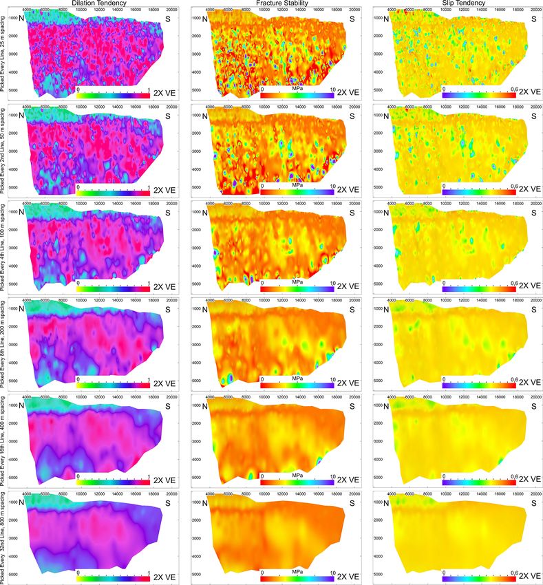
1262                      E. A. H. Michie et al.: A case study from the Horda Platform, with implications for CO2 storage

2008; Bretan et al., 2011; Miocic et al., 2019; Kayolytė et al.,    East, in the northern Horda Platform (Fig. 2). The northern
2020).                                                               Horda Platform is a 300 km by 100 km, N–S elongated struc-
   Where clay or shale layers are present within a succes-           tural high along the eastern margin of the northern North
sion, during faulting, these layers can either be juxtaposed         Sea (Færseth, 1996; Whipp et al., 2014; Duffy et al., 2015;
against the reservoir layer or become entrained into a fault,        Mulrooney et al., 2020; Fig. 2). Many deep-seated, west-
either as a smear or as a gouge (Allan, 1989; Knipe, 1992;           dipping basement faults occur within the Horda Platform,
Lindsay et al., 1993; Yielding et al., 1997). A shale smear          generating several half-graben bounding fault systems with
has been described as an abrasive shale veneer that forms a          kilometre-scale throws (Badley et al., 1988; Yielding et al.,
constant thickness down the fault (Lindsay et al., 1993). A          1991; Færseth 1996; Bell et al., 2014; Whipp et al., 2014).
fault gouge, or phyllosilicate framework fault rock (PFFR),             Two first-order, thick-skinned faults occur within the
is used to describe fault rocks that entrain clay within the         Smeaheia site: the VFZ and the Øygarden Fault Complex
fault zone, creating mixing with framework grains (Fisher            (ØFC) (Fig. 2), which bound an east-tilting half graben fol-
and Knipe, 1998). Both mechanisms have the ability to cre-           lowing a roughly north–south trend. The focus of this study
ate a barrier to fluid flow. Hence, fault seal analysis is tra-      is the VFZ, bounding the gently dipping three-way closure
ditionally completed by a combination of juxtaposition seal          Alpha prospect in its footwall (Figs. 2, 3). It is located 20 km
analysis, i.e. creating Allan diagrams (Allan, 1989), identi-        to the east of the Tusse Fault: a half-graben bounding, sealing
fying areas where there may be communication across the              fault allowing for the accumulation of hydrocarbons in Troll
fault, specifically in areas of sand–sand juxtapositions. This       East.
is then followed by a prediction of the fault rock composi-             Smaller-scale, thin-skinned northwest–southeast-striking
tion by use of various industry-standard algorithms, e.g. the        faults are also recorded at the Smeaheia site (Mulrooney
shale smear factor (SSF; Lindsay et al., 1993; Færseth, 2006)        et al., 2020). These faults only affect post-Upper Triassic
and the shale gouge ratio (SGR; Yielding et al., 1997). In this      stratigraphy and have low throws of less than 100 m (Fig. 3).
contribution, we focus on the SGR. This algorithm uses the           These faults are associated with Jurassic to Cretaceous rift-
proportion of clay (VClay or VShale ) that has moved past a          ing, which also caused reactivation of the Permo-Triassic
point on the fault to calculate the amount of clay within the        basement-involved faults (Færseth et al., 1995; Deng et al.,
fault rock:                                                          2017). However, these smaller-scale faults are not the focus
         P                                                           of this study.
            (VClay × 1z)                                                This study focuses on the Sognefjord and Fensfjord for-
SGR =                     ,                                  (1)
               throw                                                 mations as storage reservoirs for CO2 (Figs. 3, 4). Both units
where 1z is the bed thickness and VClay is the volumetric            lie within the middle–upper Jurassic Viking Group. These
clay fraction (Yielding et al., 1997). A higher SGR gener-           units represent stacked saline aquifers at this location. They
ally corresponds to an increase in phyllosilicates entrained         are composed of coastal to shallow marine deposits domi-
into the fault (e.g. Foxford et al., 1998; Yielding, 2002; van       nated by sandstones with finer-grained interlayers (Dreyer
der Zee and Urai, 2005). Hence, a higher capillary threshold         et al., 2005; Holgate et al., 2013; Patruno et al., 2015). Of
pressure is likely, which is predicted to retain a higher hy-        these, the Sognefjord Formation at the top of the stacked
drocarbon column held back by the fault (e.g. Yielding et al.,       aquifer offers the best properties. It occurs at approximately
2010). Hence, the next step in a fault seal analysis workflow        1200 m depth in the Alpha prospect and has a permeability
is to predict the column that can be held back by the fault          of 440–4000 mD and a porosity of 30 %–39 % (Statoil, 2016;
(e.g. Sperrevik et al., 2002; Bretan et al., 2003; Yielding et       Ringrose et al., 2017; Mondol et al., 2018). The Sognefjord
al., 2010). For applicability in CO2 storage, these calibrations     Formation is capped by deep marine, organic-rich mudstones
would need to be altered to take into consideration the differ-      of the Draupne Formation, as well as deep water marls, car-
ent densities, wettability and interfacial tension (Bretan et al.,   bonates and shaley units in the Cromer Knoll and Shetland
2011; Miocic et al., 2019; Kayolytė et al., 2020). However,         groups above the base Cretaceous unconformity (Nybakken
for simplicity, this paper focuses on how interpretation influ-      and Bäckstrøm, 1989; Isaksen and Ledjie, 2001; Kyrkjebø
ences the juxtaposition of sand bodies and calculated SGR,           et al., 2004; Justwan and Dahl, 2005; Gradstein and Waters,
rather attempting to predict any column heights, due to the          2016; Fig. 4).
implicit uncertainties that are imposed by the CO2 –water–              The Alpha prospect has been drilled for exploration pur-
rock systems.                                                        poses, due to hypothesized hydrocarbon migration scenarios,
                                                                     into the Smeaheia site (Goldsmith, 2000); however, well data
                                                                     from the Alpha prospect (32/4-1) have recorded no oil shows,
2   Study area                                                       indicating that no hydrocarbon migration has occurred into
                                                                     the Smeaheia site (32/4-1 T2 final well report 1997). As a re-
The Smeaheia site (see Mulrooney et al., 2020, and refer-            sult, the Smeaheia site has been assessed for the potential for
ences therein) is located approximately 40 km northwest of           CO2 storage in a saline aquifer, as it fulfils requirements for
the Kollsnes processing plant, and around 20 km east of Troll

Solid Earth, 12, 1259–1286, 2021                                                        https://doi.org/10.5194/se-12-1259-2021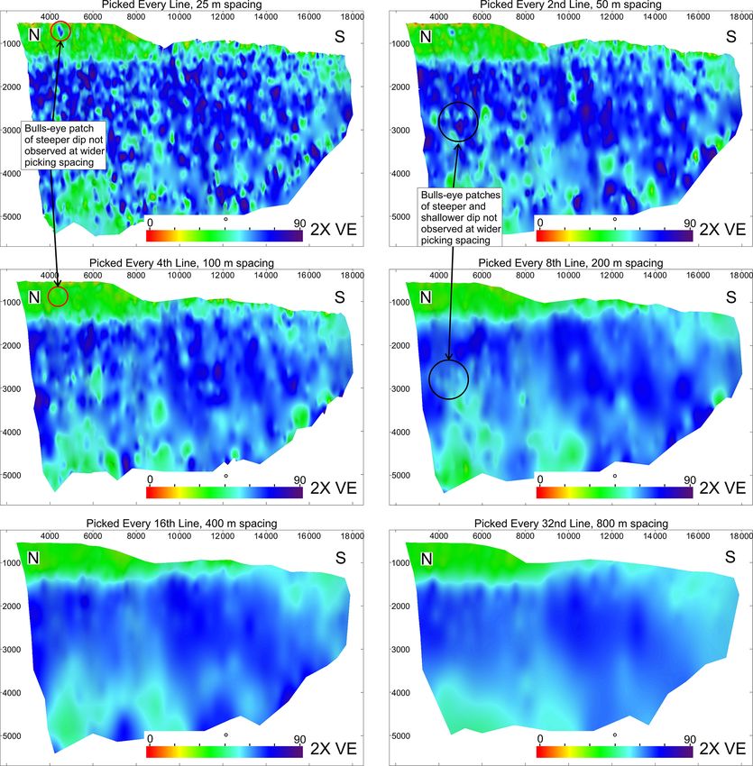
E. A. H. Michie et al.: A case study from the Horda Platform, with implications for CO2 storage 1263
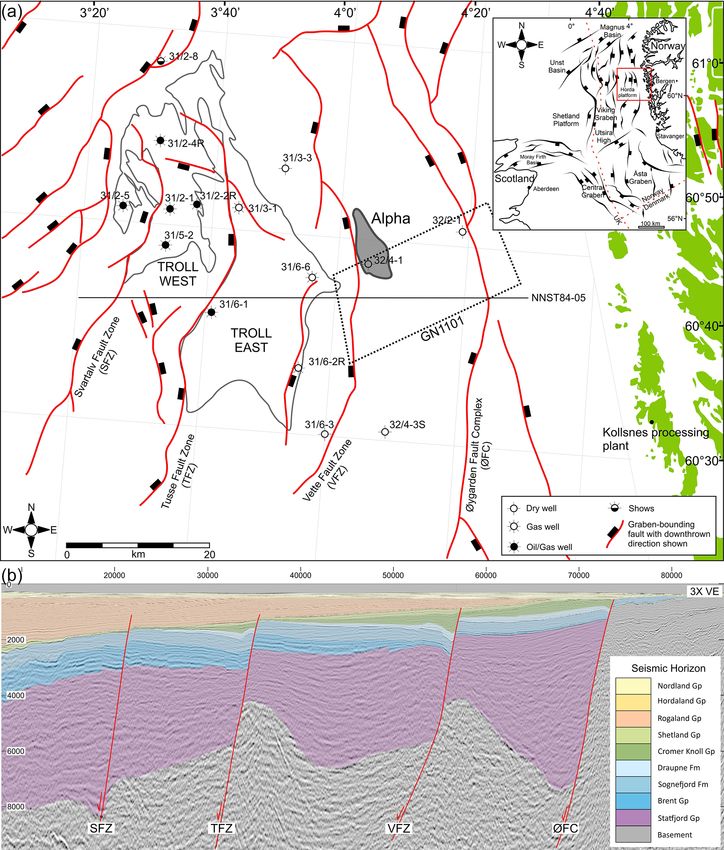
Figure 2. (a) Location of the Smeaheia site within the Horda platform, indicated by the Alpha prospect, partially covering the GN1101
survey. Graben-bounding faulting is shown, along with the hydrocarbon discovery of the Troll field. The 3-D survey used in the analysis
is outlined by a dashed black line: GN1101. Wells used in the analysis are shown. Norwegian license blocks are shown. The Norwegian
coastline outlined in green with the Kollsnes processing plant highlighted for reference, modified from Norwegian Petroleum Directorate
Fact Maps (http://factmaps.npd.no/factmaps/3_0/, last access: July 2020). Inset: location of the Horda Platform in relation to the North Sea,
Norwegian and Scottish coastline. Main structural elements are shown, such as basin-bounding faults, main basins and structural highs. After
Mulrooney et al. (2020). (b) Regional cross section across the northern Horda Platform, from 2-D seismic NNST84-05, the location of the
seismic section marked in panel (a).
substantial datasets, minimal influence on nearby production of fault that is observed in the GN1101 survey is analysed.
sites and proximity to infrastructure. The GN1101 3-D survey is a time-migrated dataset that has
subsequently been depth-converted using a simple velocity
model that has been created using quality-controlled time–
3 Methodology depth curves from 15 wells from the Troll and Smeaheia
area: 31/2-1, 31/2-2R, 31/2-4R, 31/2-5, 31/2-8, 31/3-1, 31/3-
Faults and horizons have been interpreted using one main 3, 31/5-2, 31/6-1, 31/6-2R, 31/6-3, 31/6-6, 32/2-1, 32/4-1 T2
3-D survey: GN1101, covering the Smeaheia area (Fig. 2). and 32/4-3 S (Fig. 2). Other wells in the area have no veloc-
However, it is important to note that this survey does not ity data. The GN1101 survey has good seismic quality with
extend far enough to the north and south to interpret the a resolution of roughly 15.75 m at the Sognefjord level, suit-
entire fault structure of the VFZ. Hence, only the section able for detailed structural interpretation. The GN1101 sur-
https://doi.org/10.5194/se-12-1259-2021 Solid Earth, 12, 1259–1286, 2021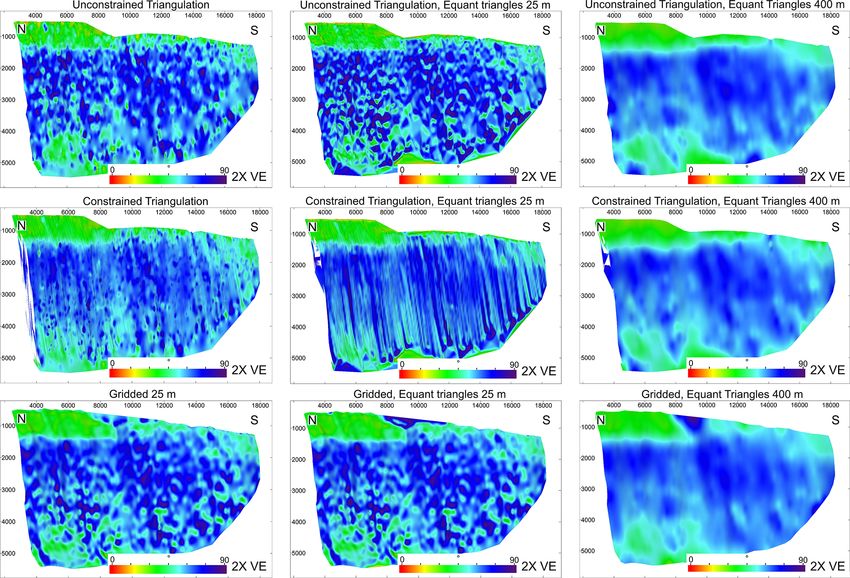
1264                      E. A. H. Michie et al.: A case study from the Horda Platform, with implications for CO2 storage

Figure 3. (a) Depth structure map of the top Sognefjord Formation. (b) Fault heave map of the top Sognefjord Formation.

vey was shot in 2011 by Gassnova SF, with an inline spacing              Interpretation and fault surface generation were performed
of 25 m and a crossline spacing of 12.5 m, covering an area           using the software T7. The fault surfaces have been created
of 442.25 km2 . Crosslines are oriented 065◦ , and inlines are        using different algorithms, illustrated in Fig. 5: (1) uncon-
oriented 155◦ . GN1101 has normal polarity and a zero-phase           strained triangulation, (2) constrained triangulation and (3)
wavelet.                                                              gridded. A combination of equant and irregular triangles of
   Five seismic horizons have been interpreted: top–Shetland          difference sizes, reflecting the picking strategy, has also been
Group, top–Cromer Knoll Group, top–Draupne Formation,                 used for each triangulation algorithm. Unconstrained trian-
top–Sognefjord Formation and top–Brent Group. The afore-              gulation generates a fault surface that triangulates fault seg-
mentioned wells with quality-controlled (QC) time–depth               ments without constraining the surface to conform to the
curves used for depth conversion have been used to aid seis-          lines between adjacent points on the same fault segment but
mic interpretation by use of well pick locations (Fig. 4).            honouring all picked points. Constrained triangulation gen-
   The VFZ has been interpreted using different line spacing          erates a surface that conforms to the points and the lines be-
in order to assess the optimum picking methodology. Faults            tween adjacent points on the same fault segment. Both un-
have been picked every 1, 2, 4, 8, 16 and 32 lines, corre-            constrained and constrained triangulations honour all data
sponding to 25, 50, 100, 200, 400 and 800 m spacing, respec-          points, and the number of data points on all fault segments
tively. Rigorous QC has been performed to ensure all data             controls the number of triangles. Gridded modelling strat-
points honour the fault surface precisely and to maintain con-        egy consists of regularly sampled points with a grid cell di-
tinuity of the fault location between each inline. Note that,         mension varying with distance between the interpreted seis-
since the GN1101 survey has been shot orthogonally to the             mic lines; hence, grid cell dimensions vary with sampling
VFZ strike trend (as is often the case, where surveys are shot        strategy. Note that no further smoothing has been applied to
perpendicular to the main fault trend to best capture their na-       any of these modelling strategies. Unconstrained triangula-
ture), only the inline orientation has been picked within this        tion is the main algorithm shown throughout, as this offers a
assessment. Adding crosslines would simply add increased              “middle-ground” modelling strategy, honouring data points
noise due to the significant picking uncertainty when a fault         but allowing some smoothing of the surface. However, the
is parallel to the seismic line, causing mismatches between           influence of algorithm choice is also assessed on any subse-
the interpretation on inlines and crosslines. Time slices us-         quent fault analysis, specifically fault dip.
ing a variance cube have also been utilized to guide interpre-           Fault attributes are calculated and mapped onto the fault
tation, as these often provide an improved visual represen-           surface at a resolution of 8 m lateral by 4 m vertical, provid-
tation of the precise location of the fault. Seismic process-         ing an optimum seismic resolution without the need to ex-
ing focused on resolving the Jurassic interval; as such, the          tend processing time. The aforementioned methods of fault
seismic quality is excellent at this location but can be sig-         surface generation are used to assess the differences in fault
nificantly more noisy elsewhere. Hence, interpreting on time          strike, dip and geomechanical attributes, when analysing
slices alone would lead to huge ambiguity, and thus they are          fault growth and fault stability. Further, fault cutoffs (inter-
used for interpretation guidance only.                                section lines on the fault surface highlighting horizon–fault

Solid Earth, 12, 1259–1286, 2021                                                           https://doi.org/10.5194/se-12-1259-2021
E. A. H. Michie et al.: A case study from the Horda Platform, with implications for CO2 storage                                     1265

Figure 4. Lithostratigraphic chart of the Horda Platform from Halland et al. (2011), with the area of interest highlighted in the red box:
the Sognefjord, Fensfjord and Krossjord formations. A seismic section is shown intersecting well 31/6-6 within the survey SG9202. Marker
horizons are shown corresponding to the lithostratigraphic column. The VShale curve from well 31/6-6 is shown, with marker horizons for
reference. The in situ stress field is shown using the combined stresses (in MPa). Pp : pore pressure. SHmin : minimum horizontal stress.
SHmax : maximum horizontal stress. Sv : vertical stress. Seismic stratigraphic column, VShale and combined stress field all have the same
depth range.

cutoffs) have been picked at each of the six fault surface it-         and to produce T-D plots used to analyse fault growth. Com-
erations, for the five mapped seismic horizons, again using            plications arise when picking fault cutoffs due to significant
different line spacing to aid with cutoff picking. Fault cutoffs       drag in the hanging wall of the VFZ. Fault cutoffs have been
have been picked using a combination of seismic slicing, at            picked honouring the drag (Fig. 6a, crosses) in order to ac-
a distance of 10 m into the footwall and hanging wall of the           curately capture the juxtapositions, as well as removing the
fault to remove any seismic noise, as well as using inlines            drag (Fig. 6a, circles), in order to accurately interpret fault
at different line spacing to accurately assess where the hori-         growth (see Jackson et al., 2017a, b).
zons intersect the fault (example shown in Fig. 6). The line              We assessed the differences in fault stability between each
spacing used is the same as that for interpreting the fault seg-       picking strategy. This is crucial when considering how the
ments; for example, a fault interpreted on every eight lines           pressure increase due to CO2 injection may influence the re-
(200 m spacing) also uses inlines at 200 m spacing to aid              activation potential of any bounding or intra-basin faults. In
with picking the cutoffs. These fault cutoffs are used to calcu-       situ stress data have been derived from an internal Equinor
late fault throw, which is mapped onto the 3-D fault surfaces,         data package (unpublished), using data from four nearby

https://doi.org/10.5194/se-12-1259-2021                                                            Solid Earth, 12, 1259–1286, 2021
1266                       E. A. H. Michie et al.: A case study from the Horda Platform, with implications for CO2 storage

                                                                         Table 1. In situ stress data used for geomechanical analysis.

                                                                                           Gradient      Stress    Depth     Direction
                                                                                         (MPa m−1 )      (MPa)       (m)     (degrees)
                                                                               SHmin          0.0146     23.07    1699.5           090
                                                                               SHmax          0.0146     23.07    1699.5           180
                                                                               Sv             0.0215     32.37    1699.5
                                                                               Pp                0.01    16.94    1699.5

                                                                         the stress orientation and faulting regime based on explo-
                                                                         ration and production wells. This area of the northern North
                                                                         Sea is found to be within a normal faulting regime with al-
                                                                         most isotropic horizontal stresses at shallower (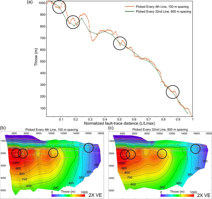
E. A. H. Michie et al.: A case study from the Horda Platform, with implications for CO2 storage                                            1267

Figure 6. (a) Inline 1224 from the GN1101 survey showing how two different fault cutoffs are created: with and without incorporating drag.
Fault cutoffs including drag simply model where the drag intersects the faults, as shown by the X on the faults for the Draupne Fm. (yellow),
Sognefjord Fm. (blue) and Brent Gp. (pink) horizons. Fault cutoffs are modelled with no drag by observing the lowest point in the hanging
wall syncline and extrapolating this point perpendicularly to the fault plane, as indicated by the dashed horizontal lines and the circles at the
intersections. (b) Oblique view of inline 1224 and the fault surface showing the footwall (FW) (solid line) and hanging wall (HW) cutoffs
(dashed lines). The two iterations of the HW cutoffs show the difference between incorporating drag and modelling the fault cutoffs with no
drag. The fault surface shows the seismic slice from 10 m into the hanging wall.

al., 2005). Note that only one well with one VShale log that               over, this analysis cannot perform fault growth analysis for
had not gone through QC, using the cursory gamma ray to                    any fault segmentation that is below seismic resolution, i.e.
VShale transform, has been used, simply as a proxy to identify             early in the fault growth phases.
how picking strategies may influence the overall fault seal
analysis, rather than to perform any rigorous fault seal analy-            4.1.1    Throw profiles
sis. If the same VShale curve is used for all instances, then any
differences identified in each scenario is simply a product of             Throw profiles highlight areas where the current fault sur-
the picking strategy used. The VShale is draped onto the fault,            face was once segmented. Here, we show throw profiles for
using the locations of picked fault cutoffs, which tie with well           the top Sognefjord along the VFZ (Fig. 7). We can observe
picks, and is used along with the throw to calculate the SGR               that the location, nature of fault interactions and number of
along the 3-D fault surface.                                               segments within initial fault array varies with picking strat-
   Note that all seismic interpretation, fault surface creation            egy (Fig. 7). Picking every line (25 m spacing) is the finest
and subsequent fault analysis was performed using the soft-                resolution in this example and is assumed to provide the best
ware T7. Complications may arise when transferring data be-                picking strategy to identify all areas of seismic-scale fault
tween different software packages. However, this added com-                segmentation. Using every line, we can interpret seven fault
plication has not been addressed within this contribution.                 segments, identified by six areas of breached relays (Fig. 7,
                                                                           highlighted by dashed vertical lines). Areas of breached re-
                                                                           lays are interpreted where significant drops in throw are ob-
4     Results                                                              served, varying from the overall throw profile and are not in-
                                                                           terpreted to be caused by other currently intersecting faults.
4.1    Fault segmentation analysis                                         Increasing the picking spacing decreases the detail required
                                                                           for accurate fault growth analysis. However, we can observe
Two main attributes are used to aid predictions of how the                 that increasing the spacing to 100 m retains the level of de-
faults have grown on the seismic scale: throw profiles and                 tail needed to identify all fault segments within this study,
strike variations. Sudden changes in throw and fault strike                that are also identified using every line spacing (Fig. 7a vs.
may indicate where initially isolated seismic-scale fault array            Fig. 7c). Beyond this spacing, the level of detail is decreased
segments subsequently linked (e.g. Cartwright et al., 1996).               causing the ability to identify some fault segmentation to be
It is important to note, however, that not all changes in fault            lost. This is most pronounced when the area of fault–fault
strike may be caused by fault linkage, and not all fault link-             intersection, and hence change in throw amplitude, is sub-
age will result in a change in fault strike. Hence, analysis               tle. This can be observed in Fig. 7d, where a picking spacing
using a combination of these fault attributes improves our un-             of 200 m loses the segmentation interpreted at approximately
derstanding of the seismic-scale fault growth history. More-               1375 m, due to the low throw variation (c. 25 m throw ampli-

https://doi.org/10.5194/se-12-1259-2021                                                                 Solid Earth, 12, 1259–1286, 2021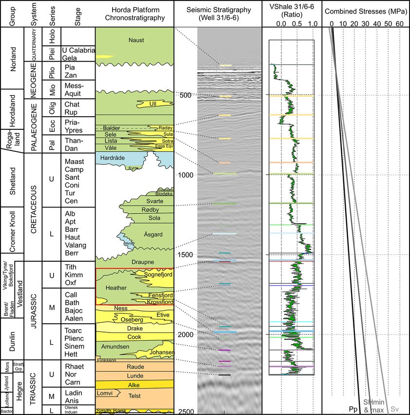
1268 E. A. H. Michie et al.: A case study from the Horda Platform, with implications for CO2 storage
tude) at this location. Using 400 and 800 m picking spacing over 40◦ , from 320 to 360◦ , in the north and over 30◦ , from
loses significant detail, such that identification of fault seg- 355 to 025◦ , in the south (Fig. 10c vs. Fig. 10a). This de-
ments is not possible for all cases where fault interactions crease in strike range with increased line spacing may limit
caused throw variations of lower than 75 m (Fig. 7e and f). the interpretation of fault growth.
Further, the precise location of interpreted fault segmentation To assess the influence of fault segmentation on fault
is often incorrect, such as that identified at 3000 m, which strike, we have highlighted the location of interpreted
should in fact be two areas of separate fault–fault intersec- seismic-scale fault segmentation, using T-D plots, on the
tions (Fig. 7e and f). fault surfaces showing strike attributes (Fig. 10). We can
To provide more detail, we show how two picking strate- see that when a fault surface is picked using every line, a
gies compare by normalizing the distance along the fault highly irregular surface is created with highly variable orien-
(Fig. 8, top) and by showing fault throw attributes and con- tations, and not every observed corrugation correlates with a
tours on the triangulated fault surfaces (Fig. 8, bottom). Since displacement minimum on the throw profile (Fig. 10a). Con-
the widest spacing that can be used without losing any seg- versely, when a fault surface is picked using 800 m line spac-
mentation detail is 100 m, we compare this example with the ing, the surface becomes overly smoothed, where no corruga-
throw profile generated by picking every 800 m line spac- tions are shown where fault segmentation is identified on the
ing (Fig. 8). We have highlighted four localities along the T-D plot. However, when every 100 m line spacing is used
fault where fault segmentation is observed on the narrower for fault picking, it appears that the majority of fault seg-
line spacing, showing displacement minima, and compared ments are also identified by fault corrugations, particularly
this to a displacement profile that does not show these dis- within the northern part of the fault (Fig. 10b). However,
placement minima when picked using a coarser line spacing some picked segmentations using T-D plots are not identi-
(Fig. 8, black circles). Hence, the locations for fault segmen- fied using corrugations, likely because not all areas of fault
tation are missed when a coarser line spacing is picked. linkage cause a change in fault strike. Further, towards the
southern half of the fault, corrugations are observed that do
4.1.2 Strike not correlate with fault segments picked using T-D plots.
While this may indicate that an overly irregular fault surface
Through examination of strike variations along the fault sur- may have been created through human error or triangulation
face, we can see a sudden change in principal strike direction method, it may also highlight potential areas of fault segmen-
shown at roughly 9000 m from the north in the fault plane tation that cannot be identified by using T-D plots alone. Al-
diagrams in Fig. 9. The strike changes from approximately ternatively, corrugations could be a product of faulting within
320 to 360◦ in the north to approximately 000 to 025◦ in the brittle and/or ductile sequences, where different types of fail-
south. Further, corrugations are observed along fault strike, ure within this sequence can create fault bends with aban-
which may be associated with fault segmentation (e.g. Fer- doned tips or splays due to strain localization and not neces-
rill et al., 1999b; Ziesch et al., 2017). However, variation sarily indicate initially isolated fault segments (Schöpfer et
in this strike trend occurs with differing picking strategies, al., 2006). Further, the corrugation size (small strike dimen-
as well as the total number of corrugations. Although the sions but large dip dimensions) may indicate potentially im-
significant change in trend observed at 9000 m in all fault plausibly low aspect ratios (see Nicol et al., 1996), and faults
plane diagrams from the north exists regardless of picking are generally recorded as decreasing in roughness with dis-
strategy, faults that are picked at 25 and 50 m line spacing placement (Sagy et al., 2007; Brodsky et al., 2011); hence,
create highly irregular surfaces, where significant strike vari- other causes for the corrugation creation may also need to be
ability is observed over relatively short distances. While this considered.
is also observed for fault surfaces picked at 100 and 200 m
line spacing, the irregularity of the surfaces is considerably
4.2 Shale gouge ratio modelling
less. However, using widely spaced picking strategies, i.e.
400 and 800 m line spacing, led to smoothing of the over-
all fault structure. Although the sudden change in strike ob- The calculated SGR is not observed to vary substantially
served at roughly 9000 m from the north remains, finer detail with picking strategy for this case study (Fig. 11a, b), even
to strike variation is lost. It is this detail that is important though substantial changes to the fault throw along strike are
when interpreting how the faults have grown by fault–fault observed (Fig. 11e), associated with differences in picking
interaction and hence identifying areas that may impact fluid strategies (as described above). Hence, the predicted shale
flow will be lost. Further, the range of strike is reduced when content within the fault does not appear to vary significantly
wider spacing is used. For example, when 800 m line spac- due to picking strategy. The shale content when a 25 m line
ing is used for seismic interpretation, the range of fault strike spacing is used is estimated to be around 40 %–50 % SGR
only varies over 20◦ , from 330 to 350◦ , in the north, and 10◦ , (high SGR values) within the Sognefjord Formation in the
from 000 to 010◦ , in the south. Conversely, when every line is footwall (Fig. 11a). The same SGR values are also calcu-
used for seismic interpretation, the range of fault strike varies lated when the fault segments and fault cutoffs are picked
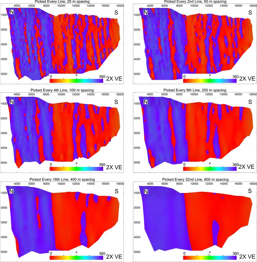
Solid Earth, 12, 1259–1286, 2021 https://doi.org/10.5194/se-12-1259-2021E. A. H. Michie et al.: A case study from the Horda Platform, with implications for CO2 storage 1269 Figure 7. Fault throw–distance plots at the top Sognefjord for each picking strategy: 25, 50, 100, 200, 400 and 800 m line spacing. Location of fault segmentation identified by changes in throw along strike is highlighted using dashed vertical lines. Those that are uncertain are indicated using a question mark. Picking using every line generates an accurate throw profile, indicating seven fault segments that occur within the GN1101 survey extents. This is also shown using a spacing of 50 and 100 m. Location and number of fault segments become increasingly uncertain when the spacing increases beyond 100 m. using every 800 m line spacing, despite large areas of drag these localities compared to when every line is picked. How- being missed (Fig. 11b). ever, the shale content in the fault may in fact be less, as the When we examine the frequency of SGR values across the calculated SGR is lower when 25 m line spacing is used for entire fault surface, we can observe that there are only minor fault cutoff modelling, which takes into consideration all ar- discrepancies between using a 25 and 800 m spacing picking eas of drag (Fig. 11d). strategy (Fig. 11c). However, when we take a closer look at the frequency of SGR values where only the Sognefjord For- 4.3 Geomechanical modelling mation is juxtaposed in the footwall and only those values where low VShale values (
1270                      E. A. H. Michie et al.: A case study from the Horda Platform, with implications for CO2 storage

Figure 8. (a) Fault throw–distance profile for the Vette fault picked at a spacing of 100 and 800 m. The x axis has been normalized for
distance along fault trace (length / length max) in order to directly compare the two scenarios. The T-D plots have been normalized due to
the restrictive size of the GN1101 survey, meaning that faults picked at increasing line spacing increments will be slightly shorter than the
last. Bottom: contoured fault throw plots displaced on a fault surface picked at every 100 m line spacing (b) and 800 m line spacing (c).
Circles highlighted in the throw–distance graph correspond to the same circles highlighted on the fault throw plots. We can observe the four
fault segments that are not recorded when a picking strategy of 800 m line spacing is used. These fault segments are recorded in the throw
profile when a narrower spacing strategy is used but are smoothed out and lost when a wider spacing strategy is used. Note that unconstrained
triangulation is used for fault surface generation.

isotropic, fault dip has a primary control on fault stability            400 and 800 m line spacing is 35◦ , compared with 15◦ dip
over fault strike. Here, we show how fault dip, and hence ge-            for faults picked at every 25 and 50 m line spacing. Further,
omechanical analysis, varies with picking strategy.                      small bulls-eye areas of steeper dip are also removed and
                                                                         smoothed when picking strategy is increased (Fig. 12, red cir-
4.3.1   Dip                                                              cles). Similarly, the steeper portion of the fault is smoothed
                                                                         as the line spacing used for picking is increased. This de-
Fault dip varies down the VFZ. There is low fault dip within             creases the range of dips and smooths any bulls-eye patches
the top 1000 m, particularly in the northern section, where the          of steeper or shallower dip (Fig. 12, black circles).
fault penetrates younger stratigraphy, specifically the Cromer              Although rigorous QC has been performed to improve
Knoll and the Shetland groups. Here, the dip decreases to ap-            continuity between each inline, there remains several places
proximately 35◦ but can be as low as 15◦ at the very top of              where slight differences in picking have occurred between
the fault (Fig. 12). The fault then steepens in dip to approxi-          lines. This human error leads to an increased irregularity of
mately 70◦ at 1500–4000 m depth, beyond which the dip de-                the fault surface, often creating these bulls-eye areas of in-
creases again to approximately 40◦ at the base of the fault.             consistent dip, associated with the triangulation algorithm
   Similar to fault strike, fault dip also varies according to           trying to honour each point along the fault segments. These
picking strategies. The shallowly dipping portion at the top             bulls-eye patches are roughly 100–200 m in size and gener-
of the fault is smoothed with increasing picking spacing,                ally occur at and below the Sognefjord level. Since fault sta-
such that the lowest dip for fault surfaces picked at every              bility is influenced by fault dip, these areas will be brought

Solid Earth, 12, 1259–1286, 2021                                                              https://doi.org/10.5194/se-12-1259-2021
E. A. H. Michie et al.: A case study from the Horda Platform, with implications for CO2 storage 1271
Figure 9. Fault plane diagrams showing fault strike attributes displayed on the fault surfaces for each picking strategy: 25, 50, 100, 200, 400
and 800 m line spacing. Fault strike is observed to vary with line spacing used for fault picking. A highly irregular fault surface is observed
when every line is used for picking, when compared to the overly smooth surface when a line spacing of 800 m is used for picking. Note that
unconstrained triangulation is used for fault surface generation.
through to geomechanical modelling. The uneven nature of for picking, where the frequency of these irregular patches
the fault surface is most severe when every inline line has is reduced. Since the fault surface is smoothed with greater
been picked (e.g. Figs. 11a and 12). The irregularity de- picking spacing (i.e. >200 m line spacing), the results for
creases with increased picking spacing. fault stability are also smoothed, reducing the range of val-
ues for each algorithms used (Fig. 14). Hence, interpretation
4.3.2 Fault stability of fault stability will vary with picking strategy and may in
fact lead to unlikely fault stability assumptions. For example,
Dip varies with picking strategy, as does the predicted fault areas where the fault is predicted to be close to failure are
stability (Fig. 13). Along fault strike, there are minor patches only observed in this study when a narrower picking strat-
where the fault is predicted to be more stable (i.e. low dila- egy is used (Figs. 12, 13). These areas are smoothed out and
tion tendency and slip tendency values or high fracture sta- not visible when a coarser picking strategy is used. However,
bility values) than the surrounding values and patches where if these areas are not a product of human error or triangula-
the fault is predicted to be less stable. These patches are most tion method, the overall stability is likely to be overestimated
apparent when every line is picked, with irregularity decreas- within this location. Patches of differing predicted fault sta-
ing in severity until every 100 to 200 m line spacing is used
https://doi.org/10.5194/se-12-1259-2021 Solid Earth, 12, 1259–1286, 20211272 E. A. H. Michie et al.: A case study from the Horda Platform, with implications for CO2 storage Figure 10. T-D plots, fault plane diagrams showing strike and rose diagrams for scenarios picked at a line spacing of 25 m (a), 100 m (b) and 800 m (c). Areas where fault segmentation has been picked using the T-D plots have been extrapolated onto the fault plane diagrams in order to assess whether areas of strike irregularities are fault corrugations highlighting areas of segmentation. Blue lines on fault plane diagrams show the level of the top Sognefjord as HW (thicker lines) and FW (thinner lines) cutoffs. Rose diagrams illustrating the orientation and range of orientation for each scenario. Note that unconstrained triangulation is used for fault surface generation. bility could also be geologically plausible due to the inherent With increasing line spacing, the fault is interpreted to be- irregularity of faults in nature. Therefore, a question is pre- come more stable as patches of steeper dip are removed. At sented regarding optimum picking strategy that retains suffi- deeper levels on the fault, patches of more and less stable cient detail but removes any data that are caused by human fault are removed with a coarser picking strategy. This cre- error and/or triangulation method. ates a fault surface where the overall stability is increased Picking strategy influences the overall interpretation of with picking strategy, as the range of predicted dilation ten- dilation tendency, fracture stability and slip tendency, and dency and slip tendency values are reduced to lower average all three stability algorithms vary with picking strategy values and a higher overall pore pressure would be required (Fig. 13). Note that the pore pressure values predicted for to cause the fault to fail (Figs. 12, 13). We can observe that fracture stability are simply used as an indication for which when every line is used for picking (25 m spacing), a large areas on the fault are more/less stable, rather than to be taken portion of the fault is in failure (i.e. the dilation tendency is as accurate pressure values that will cause the fault to reac- over 1; Fig. 14). However, the dilation tendency is reduced tivate. Fault stability varies along fault strike and down fault as the line spacing is increased. The smoothing of the fault dip, associated with varying dip attribute values (as previ- when picked at a 800 m line spacing is reflected in the nar- ously described in Sect. 4.3.1). At the top of the fault, dip rower range in predicted dilation tendency values (Fig. 14). is low such that the fault stability is interpreted to be high. A similar finding has also been recorded by Tao and Alves Solid Earth, 12, 1259–1286, 2021 https://doi.org/10.5194/se-12-1259-2021
E. A. H. Michie et al.: A case study from the Horda Platform, with implications for CO2 storage                                       1273

Figure 11. Influence of picking strategy on the predicted SGR. (a, b) Fault plane diagrams showing the predicted SGR at low VShale (
1274                      E. A. H. Michie et al.: A case study from the Horda Platform, with implications for CO2 storage

Figure 12. Fault plane diagrams showing fault dip attribute displayed on the fault surfaces for each picking strategy: 25, 50, 100, 200, 400
and 800 m line spacing. Fault dip is observed to vary with line spacing used for fault picking. A highly irregular fault surface is observed
when every line is used for picking, when compared to the overly smooth surface when a line spacing of 800 m is used for picking. Note that
unconstrained triangulation is used for fault surface generation.

terpretation, affect these analyses? Up until recently, no pa-          quired. This sampling interval would in fact be much higher
pers have documented any optimum sampling strategies for                if the entire length of the fault is used (approximately 50 km),
fault interpretation in order to make sure all fault details have       advocating for up to 1500 m spacing. However, neither of the
been captured at an ideal resolution (Tao and Alves, 2019).             suggested line spacings would be sufficient to capture all de-
Tao and Alves (2019) documented an optimum sampling in-                 tails within this study, as shown by the overly smoothed fault
terval / fault length ratio (δ) parameter, where the longer the         surface and T-D plots when picked at either 400 m or 800 m,
fault, the shorter the sampling distance required. A δ value            which do not capture any of the inherent irregularity or seg-
of 0.03 is suggested for faults that are over 3.5 km in length          mentation that occur along the fault.
(as in this example), i.e. measurements at
E. A. H. Michie et al.: A case study from the Horda Platform, with implications for CO2 storage                                          1275

Figure 13. Fault plane diagrams showing the fault reactivation potential, specifically dilation tendency, fracture stability and slip tendency
for each picking strategy: 25, 50, 100, 200, 400 and 800 m line spacing. Different conclusions regarding fault stability occur due to differing
picking strategies. Overall, the stability of the fault is observed to increase with increasing picking strategies. Note that unconstrained
triangulation is used for fault surface generation.

https://doi.org/10.5194/se-12-1259-2021                                                                Solid Earth, 12, 1259–1286, 2021
1276                      E. A. H. Michie et al.: A case study from the Horda Platform, with implications for CO2 storage

Figure 14. (a–c) Plots showing dilation tendency with depth, for scenarios with a line spacing of 25 m (a), 100 m (b) and 800 m (c). Colour
intensity reflects the frequency of those values, where blue is 1 % and red is 100 % frequency. (d) Histogram showing frequency of dilation
tendency for scenarios picked with a line spacing of 25 m (red), 100 m (orange) and 800 m (green). Note that when every line is picked, a
large portion of the values are above 1 (i.e. in failure). Dilation tendency values and their range decrease as the spacing decreases.

fault reactivation. On the contrary, when fault segments are            irregular surface is created when every line is picked. The
picked using every crossing line, a combination of human                smoothing increases as spacing increases. Hence, we sug-
error and/or triangulation method leads to an irregular fault           gest a line spacing for fault segment picking of 100 m (every
surface with bulls-eye areas of differing fault attribute val-          fourth line in this example) to most accurately capture fault
ues. This therefore leads to potential interpretation inaccu-           surface detail for all fault analyses but smooth any severe ir-
racies when fault stability analysis is performed. Suggest-             regularities between interpreted segments. Three factors are
ing an accurate picking strategy is therefore a balance be-             guiding this recommendation: time invested vs. details cap-
tween smoothing the fault surface to remove irregularities              tured and avoiding noise (irregularity) from individual fault
caused by human error and incorporating geological irregu-              segments (Fig. 15). In terms of an optimum sampling inter-
larities, for the most accurate fault analyses to be performed          val / fault length ratio (δ) parameter, the suggested 100 m line
in the shortest amount of time invested. It is also important           spacing correlates to a δ value of 0.007 if only the extents
to consider further smoothing caused by seismic resolution,             of the GN1101 survey are used (Table 2). Note, however,
since seismic data cannot capture all irregularities within a           that this suggested line spacing is specific to this case study
fault zone such as jogs and asperities. Hence, an optimum               and is likely to be different for varying sized faults, differ-
line spacing will also hinge on the limit of seismic resolu-            ent tectonic regimes, fault complexity and seismic resolution,
tion. Smoothing is also ingrained in the chosen triangulation           as well as potentially varying due to human error and level
method for fault surface creation (Fig. 1).                             of QC. Moreover, it could be argued that a best-fit model
   Faults observed in the field are often recorded as being             might prove to be adequate for analysis such as fault stabil-
highly irregular, particularly in mechanically heterogeneous            ity; hence, using every inline is not suggested as the optimum
successions, with asperities observed along strike and down             strategy for such analysis. Specifically, an over irregular fault
dip (e.g. Peacock and Xing, 1994; Childs et al., 1997). How-            may lead to the assumption that only bulls-eye areas of the
ever, the inherent imprecise nature of human picking from               fault may be reactivated; however, any reactivation is likely
one line to the next often creates severely uneven fault sur-           to influence portions of the fault between each of these bulls-
faces, despite rigorous QC (Fig. 15). We can see that the most          eye patches. However, the degree of best fit is key to this type

Solid Earth, 12, 1259–1286, 2021                                                            https://doi.org/10.5194/se-12-1259-2021
You can also read