Last interglacial (MIS 5e) sea-level proxies in southeastern South America
←
→
Page content transcription
If your browser does not render page correctly, please read the page content below
Earth Syst. Sci. Data, 13, 171–197, 2021
https://doi.org/10.5194/essd-13-171-2021
© Author(s) 2021. This work is distributed under
the Creative Commons Attribution 4.0 License.

                   Last interglacial (MIS 5e) sea-level proxies in
                           southeastern South America
           Evan J. Gowan1,2 , Alessio Rovere2 , Deirdre D. Ryan2 , Sebastian Richiano3 , Alejandro Montes4,5 ,
                                     Marta Pappalardo6 , and Marina L. Aguirre7,8
           1 Alfred    Wegener Institute, Helmholtz Centre for Polar and Marine Research, Bremerhaven, Germany
                                       2 MARUM, University of Bremen, Bremen, Germany
          3 Instituto Patagónico de Geología y Paleontología, IPGP CENPAT CONICET, Puerto Madryn, Argentina
       4 Antártida e Islas del Atlántico Sur, Instituto de Ciencias Polares, Ambiente y Recursos Naturales, Universidad

                                Nacional de Tierra del Fuego, Ushuaia, Tierra del Fuego, Argentina
                   5 Laboratorio de Geomorfología y Cuaternario, Centro Austral de Investigaciones Científicas

                                            (CADIC-CONICET), Ushuaia, Argentina
                                   6 Department of Earth Sciences, University of Pisa, Pisa, Italy
                  7 CONICET, Consejo Nacional de Investigaciones Científicas y Técnicas, La Plata, Argentina
                8 Facultad de Ciencias Naturales y Museo (FCNyM), Universidad Nacional de La Plata (UNLP),

                                                        La Plata, Argentina
                      Correspondence: Evan J. Gowan (evan.gowan@awi.de, evangowan@gmail.com)

                                 Received: 21 August 2020 – Discussion started: 10 September 2020
                       Revised: 9 December 2020 – Accepted: 10 December 2020 – Published: 28 January 2021

      Abstract. Coastal southeast South America is one of the classic locations where there are robust, spatially ex-
      tensive records of past high sea level. Sea-level proxies interpreted as last interglacial (Marine Isotope Stage 5e,
      MIS 5e) exist along the length of the Uruguayan and Argentinian coast with exceptional preservation especially
      in Patagonia. Many coastal deposits are correlated to MIS 5e solely because they form the next-highest ter-
      race level above the Holocene highstand; however, dating control exists for some landforms from amino acid
      racemization, U/Th (on molluscs), electron spin resonance (ESR), optically stimulated luminescence (OSL),
      infrared stimulated luminescence (IRSL), and radiocarbon dating (which provides minimum ages). As part of
      the World Atlas of Last Interglacial Shorelines (WALIS) database, we have compiled a total of 60 MIS 5 proxies
      attributed, with various degrees of precision, to MIS 5e. Of these, 48 are sea-level indicators, 11 are marine-
      limiting indicators (sea level above the elevation of the indicator), and 1 is terrestrial limiting (sea level below
      the elevation of the indicator). Limitations on the precision and accuracy of chronological controls and elevation
      measurements mean that most of these indicators are considered to be low quality. The database is available at
      https://doi.org/10.5281/zenodo.3991596 (Gowan et al., 2020).

1   Database and literature overview                              interstadial events when sea level reached a relative high-
                                                                  stand, MIS 5c and MIS 5a, but they have lower sea-level
During Marine Isotope Stage (MIS) 5e (about 130–115 ka),          peaks (−24 to +1 m and −22 to +1 m, respectively) than
global sea level was 5–9 m higher than at present (Kopp           MIS 5e (Creveling et al., 2017). In order to infer the ge-
et al., 2009; Dutton and Lambeck, 2012; Rovere et al.,            ometry of ice sheets during MIS 5, a global compila-
2016). MIS 5e represents one substage within MIS 5 (about         tion called the World Atlas of Last Interglacial Shorelines
130–71 ka), which is defined by relative peaks and troughs        (WALIS) database (https://warmcoasts.eu/world-atlas.html,
of deep sea benthic δ 18 O proxy records (Emiliani, 1955;         last access: 20 January 2021) has been created to document
Shackleton, 1969) (Fig. 1). Within MIS 5, there are two

Published by Copernicus Publications.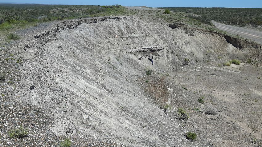
172                                                                E. J. Gowan et al.: MIS 5e sea level in southeast South America

                                                                         matic conditions and minimal erosion, there is exceptional
                                                                         preservation of beach ridges and other relic Quaternary and
                                                                         Pliocene deposits along the entire coast, and they show re-
                                                                         markable continuity. North of Patagonia, in Buenos Aires
                                                                         Province, Pleistocene marine and estuary sediments have
                                                                         also been found (e.g. Aguirre and Whatley, 1995). For the
                                                                         WALIS database, we have only included sea-level indicators
                                                                         with sufficient depositional context to confidently assign an
Figure 1. Definition of marine isotope stages. The black line is the
                                                                         indicative range (aside from estuary deposits, which are here
LR04 benthic δ 18 O stack (Lisiecki and Raymo, 2005). The MIS            considered marine-limiting data points), sufficient elevation
stages denoted in red are warm interglacial and interstadial periods,    information to infer the paleo sea level, and chronological
while blue areas are colder glacial and stadial periods. The MIS 5       control that provides some confidence that the indicator is
substage boundaries are from Otvos (2015), while the others are          MIS 5 in age. The indicative range is the elevation range,
defined by Lisiecki and Raymo (2005).                                    relative to a fixed water level (i.e. mean sea level) in which a
                                                                         landform, deposit, or biological material will be found (Shen-
                                                                         nan, 2015).
MIS 5e sea-level indicators and proxies following a stan-                   Geological indicators of multiple past sea-level highstands
dardized data template. Our database is open access and                  in Argentina (specifically Patagonia) were first measured and
available at https://doi.org/10.5281/zenodo.3991596 (Gowan               described in detail by Darwin (1846) in The Voyage of the
et al., 2020), and descriptions of each database field can               Beagle. Darwin presented six cross sections of marine ter-
be found at https://doi.org/10.5281/zenodo.3961544 (Rovere               races, though only three of them had levels that are po-
et al., 2020b). Our database of southeastern South Amer-                 tentially last interglacial in age (most are reported at much
ican paleo-sea-level proxies incorporates geologically con-              higher elevations). Darwin remarked on how the elevation of
strained features with sufficient elevation and geological con-          different terraces seemed to be nearly the same along the en-
text to infer past sea-level position. The literature survey cov-        tire Patagonian coast and concluded that their formation was
ers Uruguay, Argentina, and the eastern portion of Tierra del            likely the result of land being uplifted. This hypothesis con-
Fuego in Chile. Published proxies exist along the entire coast           tinues to be favoured by many researchers working on Ar-
(Fig. 2).                                                                gentinian sea level (e.g. Pedoja et al., 2011; Isla and Angulo,
   Due to uncertainty in the age constraints, many of the fea-           2016).
tures in this paper are assigned to MIS 5, rather than specifi-             The commonly used nomenclature of Patagonian terrace
cally to MIS 5e. However, due to the differences in sea-level            levels was proposed by Feruglio (1950). In total, Feruglio
height between the successive substages of MIS 5, in the                 (1950) identified and correlated six distinct terraces (I to VI,
absence of evidence for tectonic effects, specifically uplift,           Table 1) on the basis of terrace elevation and fossil mol-
we infer that any sea-level record that has been attributed to           lusc assemblage. Subsequent studies correlated Terrace V to
MIS 5 corresponds to MIS 5e. This work is similar to other               MIS 5 (Codignotto et al., 1988; Rutter et al., 1989, 1990;
studies where there are multiple highstand records for MIS 5             Rostami et al., 2000). Feruglio’s terrace nomenclature and
present, in that MIS 5e features are expected to be those at the         correlations have continued to be used by subsequent au-
highest elevation (Lambeck and Chappell, 2001; Potter et al.,            thors. The next major set of studies on past Patagonian sea
2004; Dumas et al., 2006; Surić et al., 2009; Moseley et al.,           level was done by Codignotto and colleagues (Bayarsky and
2013), MIS 5e features are expected to be those at the high-             Codignotto, 1982; Codignotto, 1983, 1984, 1987), which
est elevation. Many of the studies on shoreline deposits de-             was summarized by Codignotto et al. (1988). Many of these
scribed in this database gave support for an MIS 5e substage             terraces were dated using radiocarbon measurements. Pre-
assignment based on comparing the abundance of species                   Holocene terraces that returned finite dates were regarded by
of molluscs to infer paleo-water temperatures (e.g. Aguirre              Codignotto et al. (1988) as belonging to the late Pleistocene.
et al., 2006; Martínez et al., 2016). We have decided in our                From the late 1980s onwards, a number of studies pre-
database to only include deposits that have numeric age con-             sented chronological constraints allowing for a more con-
trol and are assigned an MIS 5 (or MIS 3; see Sect. 4.6) age             fident MIS 5 assignment. Techniques used to date MIS 5
by the original authors and to only use faunal evidence if used          shorelines in Argentina include amino acid racemization
by the original authors. We acknowledge that due to the im-              (Rutter et al., 1989, 1990; Aguirre et al., 1995; Schellmann,
precision of the dating methods applied to the deposits in the           1998), electron spin resonance (Radtke, 1989; Rutter et al.,
entire study area, they may represent an MIS 5a or MIS 5c                1990; Schellmann, 1998; Schellmann and Radtke, 2000), and
highstand or even Holocene or pre-MIS 5 highstands.                      U/Th on mollusc shells (Radtke, 1989; Schellmann, 1998;
   Patagonian Argentina was one of the first places in the               Isla et al., 2000; Rostami et al., 2000; Bujalesky et al., 2001;
world where multiple distinct indicators of past sea-level               Pappalardo et al., 2015). These studies provide the bulk of the
highstands were observed (Darwin, 1846). Due to the cli-                 confidently assigned MIS 5 sea-level proxies in the database.

Earth Syst. Sci. Data, 13, 171–197, 2021                                                  https://doi.org/10.5194/essd-13-171-2021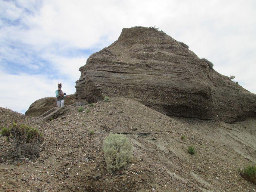
E. J. Gowan et al.: MIS 5e sea level in southeast South America                                                                    173

Figure 2. MIS 5 sea-level indicators along the southeastern South America coastline (black-outlined circles).

Table 1. Terrace levels identified by Feruglio (1950).                  into seven zones and measured elevations of changes in slope
                                                                        in the topography, which they interpreted as past sea-level
    Terrace   Elevation    Type location                                highstands (shoreline angles). They reported up to nine slope
    name           (m)                                                  angles in these zones. Their interpreted MIS 5 shoreline
    VI            8–10     Comodoro Rivadavia                           (named T1) indicates that there is spatial variability in the
    V            15–18     Mazarredo                                    elevation.
    IV           35–40     Escarpado Notre (Puerto Deseado)
    III          70–80     Camarones                                    2   Sea-level indicators
    II         104–140     Cabo Tres Puntas (Puerto Deseado)
    I          170–186     Cerro Laciar                                 The descriptions of types of sea-level proxies found in Ar-
                                                                        gentina are found in Table 2. The sea-level indicators include
                                                                        beach deposits (e.g. Fig. 3), beach ridges (e.g. Fig. 4), paleo-
                                                                        lagoonal deposits, and marine terraces. In addition, there are
  The most recent review of past sea level in Argentinian
                                                                        marine-limiting estuary deposits.
Patagonia was by Pedoja et al. (2011). They split the coast

https://doi.org/10.5194/essd-13-171-2021                                                   Earth Syst. Sci. Data, 13, 171–197, 2021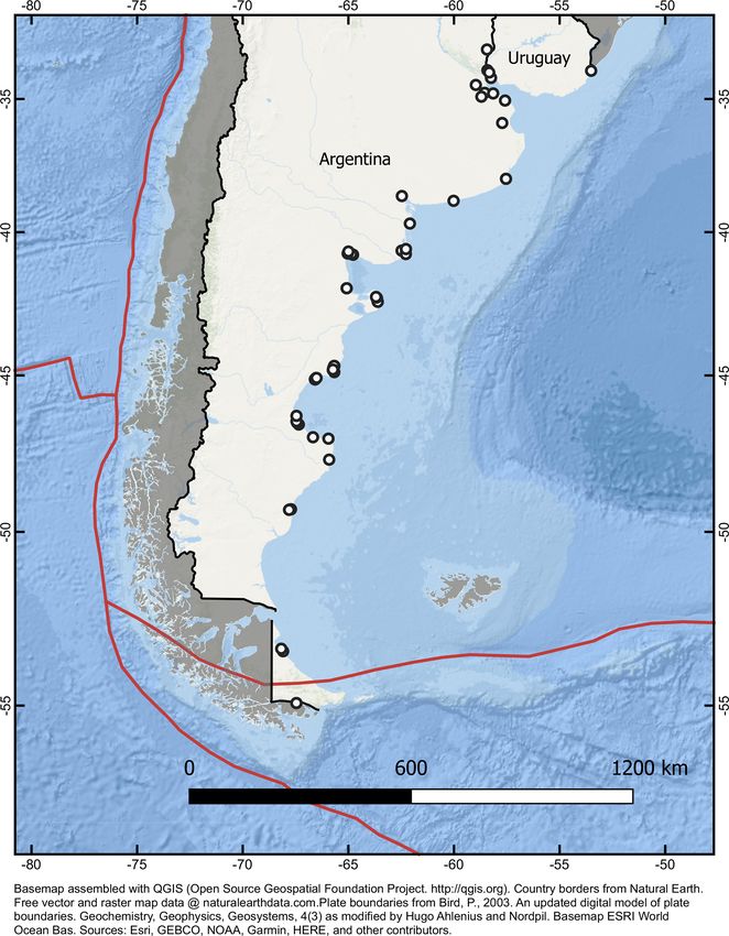
E. J. Gowan et al.: MIS 5e sea level in southeast South America

                                                                                                                                                                                                                                                          https://doi.org/10.5194/essd-13-171-2021
                                                                  Table 2. Different types of relative sea level (RSL) indicators reviewed in this study. RWL denotes reference water level, and IR denotes indicative range.
                                                                   Name of RSL       Description of RSL indicator                                           Description of RWL          Description of IR                         Indicator
                                                                   indicator                                                                                                                                                      reference(s)
                                                                   Marine            From Pirazzoli (2005): “any relatively flat surface of marine          (Storm wave swash height    Storm wave swash                          Mauz et al. (2015),
                                                                   terrace           origin”. Definition of indicative meaning from Rovere et al.           + breaking depth) / 2       height–breaking depth                     Rovere et al. (2016)
                                                                                     (2016).
                                                                   Beach     de-     From Mauz et al. (2015): “Fossil beach deposits may be                 (Ordinary berm + breaking   Ordinary berm–breaking depth              Mauz et al. (2015),
                                                                   posit             composed of loose sediments, sometimes slightly cemented.              depth) / 2                                                            Rovere et al. (2016)
                                                                   or beachrock      Beachrocks are lithified coastal deposits that are organized in
                                                                                     sequences of slabs with seaward inclination generally between
                                                                                     5◦ and 15◦ .” Definition of indicative meaning from Rovere et al.
                                                                                     (2016).
                                                                   Beach ridge       From Otvos (2000): “stabilized, relict intertidal and supratidal,      (Storm wave swash height    Storm wave swash                          Otvos (2000),
                                                                                     eolian and wave-built shore ridges that may consist of either          + ordinary berm) / 2        height–ordinary berm                      Rovere et al. (2016)
                                                                                     siliciclastic or calcareous clastic matter of a wide range of clasts
                                                                                     dimensions, from fine sand to cobbles and boulders.” Definition
                                                                                     of indicative meaning from Rovere et al. (2016).
                                                                   Lagoonal          Lagoonal deposits consist of silty and clayey sediments, fre-          (Mean lower low water       Mean lower low water–modern               Rovere et al. (2016),
                                                                   deposit           quently characterized by the presence of brackish or marine            + modern lagoon depth)      lagoon depth                              Zecchin et al. (2004)
                                                                                     water fauna (Rovere et al., 2016). Usually, lagoon sediments           /2
                                                                                     are horizontally laminated (Zecchin et al., 2004). Definition of

                                                                                                                                                                                                                                                          Earth Syst. Sci. Data, 13, 171–197, 2021
                                                                                     indicative meaning from Rovere et al. (2016).
                                                                   Estuary           From Perillo (1995): “An estuary is a semi-enclosed costal body        < Highest astronomical      The upper limit of estuary deposits is    Perillo (1995)
                                                                   deposit           of water that extends to the effective limit of tidal influence,       tide (HAT)                  the highest astronomical tide, but the
                                                                                     within which sea water entering from one or more free con-                                         lower limit is bounded bathymetry. As
                                                                                     nections with the open sea, or any other saline coastal body of                                    a result, an estuary deposit can only
                                                                                     water, is significantly diluted with fresh water derived from land                                 be used as a marine-limiting indicator,
                                                                                     drainage, and can sustain euryhaline biological species from ei-                                   with an uncertainty range that is HAT–
                                                                                     ther part or the whole of their life cycle.”                                                       MSL (mean sea level).
174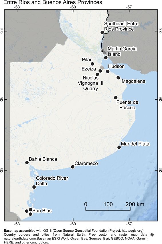
E. J. Gowan et al.: MIS 5e sea level in southeast South America 175
apply the difference between the high tide level and median
level to the elevation uncertainty.
In cases where elevations are reported as being rela-
tive to high tide, we provide a correction to make the
reference to mean sea level. The tide statistics are taken
from the Servicio de Hidrografía Naval website (http://www.
hidro.gov.ar/oceanografia/Tmareas/Form_Tmareas.asp, last
access: 20 January 2021). The tide tables only report the
predicted astronomical component of the tide and do not
take into account meteorological or steric components (Pap-
palardo et al., 2019). This will introduce an uncertainty of
unknown magnitude to all data referenced to tidal datums
from these sources (see Sect. 3).
One of the challenges when making this database is that
stratigraphic descriptions and interpretations of depositional
environment are not stated. The beach ridge deposits of
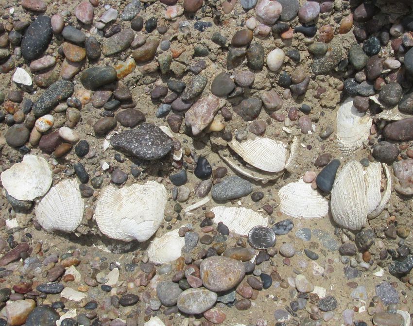
Figure 3. MIS 5 beach deposit near Caleta Olivia. The photo was Patagonia are typically composed of gravel (Tamura, 2012),
taken on the front side of the beach deposit. and deposition via wave action is certain. The beach ridges
in Patagonia are typically interpreted as raised storm berms.
The presence of marine shells within terrace beds allows
for the inference that they are marine in origin. However,
the lack of descriptions has prompted the assignment of low
quality scores to some of these indicators. Studies with de-
tailed stratigraphic context and, as a consequence, relatively
high quality scores can be found in Schellmann (1998) and
Rabassa et al. (2008). A summary of the indicators, along
with quality assessment, is shown in Table 3.
3 Elevation measurements
Most of the reviewed studies report elevations measured
Figure 4. MIS 5 beach ridge deposit near Camarones. The photo
by barometric altimeter or do not report an elevation mea-
illustrates the back side of the beach ridge, with the sea located on surement method (Table 6). Rostami et al. (2000) state that
the left side of the photo. there is a strong suspicion that elevation in some studies
may have just taken the value from Feruglio (1950) (which
was likely derived from topography maps and Jacob’s staff
measurements), rather than from direct measurement. Pap-
For most of the data presented in this database, no indica- palardo et al. (2019) did a further review of the vertical un-
tive meaning or modern analogue was provided in the orig- certainties of Argentinian sea-level indicators and stated that
inal studies. As a result, we use the IMCalc tool (Lorscheid problems with misidentification of sea-level indicators and
and Rovere, 2019) to calculate the indicative range. IMCalc poor-quality elevation measurements hamper accurate as-
uses the definitions from Table 2 plus global wave and tidal sessments of paleo sea level. They also state that even within
models to estimate the indicative range at the location of the the same region, several studies disagree on what paleo sea
sample. level was during MIS 5, due to methodological differences in
At multiple locations in northern Argentina, two Pleis- measuring elevation. The elevation measurements for previ-
tocene or older estuary deposits are identified (Fig. 7). One ous studies were often made at the elevation of the shell sam-
is highly cemented and has not been analyzed by any nu- ples used for dating, rather than made measuring the thick-
merical geochronological method. The second unit, overly- ness of the geological unit that would provide a more robust
ing the highly cemented deposit, has returned finite radio- estimate of the true paleo-sea-level range. As an example
carbon dates. The interpretation of these radiocarbon dates (Table 1 in Pappalardo et al., 2019), at Camarones, estimates
is elaborated in Sect. 4. The estuary deposits are regarded as of MIS 5 sea level ranged between 7.5 and 17 m in different
minimum-limiting indicators, as there is no limit to the depth studies.
at which they can be found (Perillo, 1995). The maximum Due to the ambiguity of elevation measurements, a high
limit is the highest astronomical tide, so it is necessary to degree of uncertainty is assigned to many sea-level indica-
https://doi.org/10.5194/essd-13-171-2021 Earth Syst. Sci. Data, 13, 171–197, 2021
176                                                              E. J. Gowan et al.: MIS 5e sea level in southeast South America

Table 3. Summary of reviewed inferred MIS 5 sea-level data. For references refer to the text.

   Site name                         Latitude    Longitude    Indicator    RSL or elevation     Dating methods      RSL         Age
                                                              Type1                    (m)                       quality2   quality2
   Southeast Entre Ríos Province     −33.060      −58.440     ML                  6.2 ± 1.6     14 C                   1          0
   Puerto de Nueva Palmira           −33.880      −58.419     ML                 12.5 ± 2.8     OSL, 14 C              1          2
   La Coronilla                      −33.900      −53.509     ML                  0.5 ± 0.5     14 C                   1          0
   Zagarzazú                         −33.966      −58.335     ML                  0.5 ± 0.5     OSL, 14 C              1          2
   Martín García Island              −34.180      −58.250     ML                  7.5 ± 1.7     14 C                   1          0
   Pilar                             −34.456      −58.968     ML                  8.0 ± 1.8     14 C                   1          0
   Ezeiza                            −34.764      −58.550     ML                  3.5 ± 0.8     OSL, 14 C              1          0
   Hudson                            −34.786      −58.149     ML                  6.0 ± 1.9     OSL                    1          2
   Nicolás Vignogna III Quarry       −34.913      −58.705     TL                  1.3 ± 3.1     OSL, 14 C              1          0
   Magdalena                         −35.062      −57.586     ML                  6.0 ± 1.7     AAR, 14 C              1          3
   Puente de Pascua                  −35.927      −57.720     ML                  3.5 ± 1.3     AAR                    1          3
   Puente de Pascua                  −35.927      −57.719     SLI                 6.8 ± 4.0     AAR                    2          3
   Mar del Plata                     −38.040      −57.540     SLI                10.3 ± 2.5     14 C                   1          0
   Bahía Blanca                      −38.680      −62.470     ML                 13.1 ± 3.7     14 C                   1          0
   Claromecó                         −38.856      −60.021     SLI                 7.0 ± 2.0     U/Th                   1          3
   Colorado River delta              −39.690      −62.090     SLI                 4.8 ± 1.8     14 C                   1          0
   San Blas                          −40.614      −62.278     SLI                 5.8 ± 3.8     14 C                   1          0
   San Blas                          −40.671      −62.482     SLI                12.4 ± 3.1     AAR                    1          1
   San Antonio Oeste                 −40.703      −65.000     SLI                 6.3 ± 2.8     ESR, U/Th              2          3
   San Antonio Oeste                 −40.772      −65.036     SLI                 8.7 ± 3.9     AAR, ESR, U/Th         2          3
   San Antonio Oeste                 −40.792      −64.861     SLI                 9.7 ± 8.6     AAR                    1          1
   San Blas                          −40.793      −62.283     SLI                 4.0 ± 3.9     AAR, ESR               2          2
   San Antonio Oeste                 −40.817      −64.782     SLI                 9.0 ± 5.5     AAR, ESR               2          3
   Puerto Lobos                      −42.008      −65.084     SLI                 8.8 ± 2.9     14 C                   1          0
   Puerto Lobos                      −42.008      −65.084     SLI                 6.8 ± 2.7     14 C                   1          0
   Caleta Valdés                     −42.313      −63.694     SLI                16.6 ± 4.2     ESR, U/Th              2          3
   Caleta Valdés                     −42.334      −63.672     SLI                15.6 ± 4.0     U/Th                   2          3
   Caleta Valdés                     −42.350      −63.650     SLI                19.1 ± 7.5     14 C                   1          0
   Caleta Valdés                     −42.395      −63.644     SLI                20.7 ± 4.4     AAR, ESR               1          3
   Caleta Valdés                     −42.484      −63.611     SLI                 9.2 ± 3.3     AAR, ESR, U/Th         1          1
   Camarones                         −44.681      −65.668     SLI                 4.8 ± 5.6     U/Th                   1          3
   Camarones                         −44.683      −65.679     SLI                 4.8 ± 1.5     U/Th                   1          3
   Camarones                         −44.693      −65.674     SLI                 6.5 ± 5.8     ESR, U/Th              1          3
   Camarones                         −44.716      −65.693     SLI                12.8 ± 3.3     ESR                    1          3
   Camarones                         −44.750      −65.720     SLI                19.1 ± 5.4     14 C                   0          0
   Camarones                         −44.806      −65.734     SLI                 7.8 ± 1.5     U/Th                   1          3
   Camarones                         −44.820      −65.740     SLI                17.8 ± 6.0     14 C                   0          0
   Camarones                         −44.890      −65.670     SLI                15.8 ± 4.0     ESR, U/Th              0          3
   Bahía Bustamante                  −45.087      −66.510     SLI                 8.4 ± 2.3     ESR                    1          3
   Bahía Bustamante                  −45.090      −66.531     SLI                12.8 ± 5.6     AAR, ESR, U/Th         1          2
   Bahía Bustamante                  −45.090      −66.531     SLI                 9.5 ± 4.9     AAR, ESR, U/Th         1          2
   Bahía Bustamante                  −45.112      −66.552     SLI                14.2 ± 3.7     ESR                    1          2
   Bahía Bustamante                  −45.113      −66.546     SLI                 5.9 ± 2.3     ESR                    3          2
   Bahía Bustamante                  −45.133      −66.589     SLI                14.2 ± 3.7     ESR                    1          3
   Bahía Bustamante                  −45.137      −66.579     SLI                 8.3 ± 2.8     AAR, ESR, U/Th         3          3
   Caleta Olivia                     −46.340      −67.461     SLI                15.5 ± 4.0     U/Th                   2          3
   Caleta Olivia                     −46.519      −67.461     SLI                15.5 ± 4.0     ESR, U/Th              2          3
   Caleta Olivia                     −46.558      −67.434     SLI                10.8 ± 8.9     AAR, ESR               1          3
   Caleta Olivia                     −46.564      −67.428     SLI                14.0 ± 8.4     AAR, ESR               1          3
   Caleta Olivia                     −46.622      −67.351     SLI                12.3 ± 4.0     14 C                   1          0
   Mazarredo                         −47.035      −66.679     SLI                12.2 ± 3.4     AAR, ESR, U/Th         1          3
   Mazarredo                         −47.080      −65.947     SLI                15.9 ± 4.0     U/Th                   0          3
   Puerto Deseado                    −47.754      −65.913     SLI                22.2 ± 7.1     AAR, ESR               1          1

Earth Syst. Sci. Data, 13, 171–197, 2021                                                   https://doi.org/10.5194/essd-13-171-2021
E. J. Gowan et al.: MIS 5e sea level in southeast South America                                                                                                                       177

Table 3. Continued.

      Site name                                   Latitude       Longitude         Indicator       RSL or elevation           Dating methods              RSL             Age
                                                                                   type1                       (m)                                     quality2       quality2
      San Julián                                 −49.310           −67.720         SLI                       7.6 ± 3.4        ESR                               1                 3
      San Julián                                 −49.316           −67.776         SLI                      15.1 ± 4.2        ESR, U/Th                         2                 3
      San Julián                                 −49.327           −67.809         SLI                       6.7 ± 3.7        ESR                               2                 3
      San Julián                                 −49.327           −67.809         SLI                       5.1 ± 2.9        ESR                               2                 3
      Northeastern Tierra del Fuego              −53.431           −68.180         SLI                      17.5 ± 5.6        14 C                              1                 0
      Northeastern Tierra del Fuego              −53.502           −68.094         SLI                      13.4 ± 3.7        AAR, U/Th                         1                 3
      Puerto Williams                            −54.936           −67.466         SLI                      11.1 ± 2.1        14 C, IRSL                        3                 3
    1 SLI – sea-level indicator; ML – marine limiting; TL – terrestrial limiting. 2 Quality ranges from 5 (excellent) to 0 (rejected). See Tables 4 and 5 for more information.

tors. An additional 20 % uncertainty (a value recommended                                      cally stimulated luminescence (OSL), infrared stimulated lu-
by Rovere et al., 2016) was added to altimetric measurements                                   minescence (IRSL), and radiocarbon methods. Marine shell
since this method is less reliable than levelling or differen-                                 fossils (Fig. 5), often still articulated, are abundant in many
tial GPS and results can vary depending on atmospheric con-                                    shoreline deposits. AAR, ESR, and U/Th techniques can
ditions. This added uncertainty is further justified as most                                   provide a confident MIS 5 age assignment provided there
altimetric measurements lack details on how they were ref-                                     has been limited chemical alteration. These methods can be
erenced to sea level. An additional source of uncertainty is                                   used to distinguish shells of MIS 5 from earlier interglacials
when a section is described, but it is not clear if the reported                               or the Holocene but lack the resolution to differentiate be-
elevation refers to the top or the bottom of the section. In                                   tween substages of MIS 5, i.e. 5e, 5c, or 5a. A wide variety
these instances, the entire thickness of the section is added to                               of bivalve and gastropod species have been used for dating,
the error. When the details of where on the outcrop or land-                                   which are listed in Table 7. Radiocarbon and, to some ex-
form the elevation was measured are not stated, the elevation                                  tent, OSL dates have been used to establish minimum ages,
error is assigned to be 20 % of the reported elevation from                                    proving that a deposit is older than the Holocene. Other abso-
the highest reported elevation. Either all elevations were re-                                 lute dating techniques, the environmental context from fauna,
ported in reference to mean sea level (often referenced to a                                   and stratigraphic position can be used to support an MIS 5
local tide gauge), or, for studies in which no sea-level da-                                   age assignment. An overview of the quality score criteria for
tum is defined, the measurements were assumed to be refer-                                     age constraints is in Table 5. In this compilation, for any site
enced to mean sea level for entry into WALIS. This definition                                  where minimum ages are the only chronological control, we
may have complications as the local “mean” sea level can                                       give a low quality assignment (i.e. zero out of five). We did
have an offset from the global mean sea level (or orthomet-                                    not include features that have no dating applied to them in
ric elevation) (Lanfredi et al., 1998; Pappalardo et al., 2019),                               WALIS, though for some locations we have noted them in
which has not been accounted for in our entries. Sites that                                    the text.
were reported from a high-tide datum have been corrected to
mean sea level using the values from nearby tidal charts (see                                  4.1     Amino acid racemization (AAR)
Sect. 2).
   In some locations, it is possible that the same outcrop is                                  The analytical procedure for AAR is reported by Rutter et al.
described by multiple studies. However, since the precise lo-                                  (1989). They reported aspartic acid and leucine values of
cations of these deposits are not always clear, each record                                    multiple species of shells, without analytical uncertainties.
is included as a separate indicator, with individual elevation                                 They did not report numerical ages, only using the values
uncertainties. Indicators for which it was not possible to de-                                 to distinguish between deposits of different ages. Aguirre
termine an exact location are included in the database, since                                  et al. (1995) reported numerical ages from AAR, calibrated
they may have some utility in future modelling studies, but                                    with Holocene shells of the same species. However, due to
are given the lowest quality score (zero). An overview of the                                  the non-linear kinematics of racemization, this approach is
quality score criteria for RSL is in Table 4.                                                  not recommended in Pleistocene shells (Clarke and Murray-
                                                                                               Wallace, 2006). In order to draw correlations, the same
                                                                                               species should be used, since the racemization is species de-
4    Dating techniques                                                                         pendent. This is not possible in many of the locations where
                                                                                               AAR samples have been reported in our study area.
MIS 5 deposits in southeastern South America have been
dated using amino acid racemization (AAR) values, electron
spin resonance (ESR), uranium–thorium dating (U/Th), opti-

https://doi.org/10.5194/essd-13-171-2021                                                                                Earth Syst. Sci. Data, 13, 171–197, 2021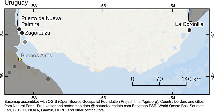
178                                                              E. J. Gowan et al.: MIS 5e sea level in southeast South America

Table 4. Quality scores for RSL, from the WALIS documentation.

                    Description                                                                        Quality rating
                    Elevation precisely measured and referred to a clear datum and RSL indicator       5 (excellent)
                    with a very narrow indicative range. Final RSL uncertainty is submetric.
                    Elevation precisely measured and referred to a clear datum and RSL indicator       4 (good)
                    with a narrow indicative range. Final RSL uncertainty is between 1 and 2 m.
                    Uncertainties in elevation, datum, or indicative range sum up to a value of be-    3 (average)
                    tween 2 and 3 m.
                    Final paleo RSL uncertainty is higher than 3 m.                                    2 (poor)
                    Elevation and/or indicative range must be regarded as very uncertain due to poor   1 (very poor)
                    measurement, description, or RSL indicator quality.
                    There is not enough information to accept the record as a valid RSL indicator      0 (rejected)
                    (e.g. marine or terrestrial limiting).

Table 5. Quality scores for age, from the WALIS documentation.

                          Description                                                            Quality rating
                          Very narrow age range, e.g. a few thousand years, that allows the      5 (excellent)
                          attribution to a specific timing within a substage of MIS 5 (e.g.
                          117 ± 2 ka
                          Narrow age range, allowing the attribution to a specific substage of   4 (good)
                          MIS 5 (e.g. MIS 5e)
                          The RSL data point can be attributed only to a generic interglacial    3 (average)
                          (e.g. MIS 5)
                          Only partial information or minimum age constraints are available      2 (poor)
                          Different age constraints point to different interglacials             1 (very poor)
                          Not enough information to attribute the RSL data point to any Pleis-   0 (rejected)
                          tocene interglacial

4.2   Electron spin resonance (ESR)                                      a number of articulated shells from a deposit in Camarones
                                                                         and showed a large spread in ages (dating to between 92–
The details of ESR dating can be found in Rutter et al. (1990)           171 ka), which demonstrated the care that must be taken in
and Schellmann and Radtke (1997, 1999). The main issue                   interpreting the results of ESR dating. Due to the uncertainty
with ESR is that mollusc shells are not a closed system to ura-          in the uranium uptake history of shells, it is not possible to
nium, so therefore it cannot be assumed that the uranium con-            use this method to distinguish between substages in MIS 5,
centration has been constant since deposition (Radtke et al.,            even if the reported ages indicate ages that are younger than
1985; Schellmann and Radtke, 1999). As a result, Schell-                 MIS 5e.
mann and Radtke (1997) recommended using the “early-
uptake” model for determining the age. Under this hypoth-                4.3 U/Th dating
esis, most of the uranium was taken up in the shell within the
first 10 000 years of deposition. Although this approach will            The U/Th dating done by Radtke (1989) was accom-
give younger ages than the commonly used “linear-uptake”                 plished using mass spectrometry. The measurements were
model, Schellmann and Radtke (1997) regarded it as being                 done at three laboratories; University of Cologne, Heidel-
more accurate. All of the ages in this database use the early-           berg University, and McMaster University. The University
uptake model. The early ESR dates (Radtke, 1989; Rutter                  of Cologne laboratory corrected for excess thorium using
et al., 1990) are not reported with an uncertainty, so we use            the formula − 232 Th × (3 ppm U/12 ppm Th) × 0.378 if the
a value of 15 % of the age, as recommended in those stud-                thorium was in excess of 0.3 ppm. This corrected value was
ies. Schellmann and Radtke (1999) tested their methods on                preferred by Radtke (1989). Rostami et al. (2000) reported

Earth Syst. Sci. Data, 13, 171–197, 2021                                                  https://doi.org/10.5194/essd-13-171-2021
E. J. Gowan et al.: MIS 5e sea level in southeast South America                                                                         179

Table 6. Measurement techniques used to establish the elevation of MIS 5 shorelines in Argentina.

      Measurement          Description                                               Typical accuracy
      technique
      Not reported         The elevation measurement technique was not reported,     20 % of the original reported elevation added to
                           most probably hand level or metered tape.                 the root mean square error
      Barometric           Difference in barometric pressure between a point of      Up to ±20 % of elevation measurement
      altimeter            known elevation (often sea level) and a point of un-
                           known elevation. Not accurate and used only rarely.
      Topographic map      Elevation derived from the contour lines on topographic   Variable with scale of map and technique used
      and digital eleva-   maps. Most often used for large-scale landforms (i.e.     to derive DEM
      tion models          marine terraces). Several meters of error are possible,
                           depending on the scale of the map or the resolution of
                           the DEM.

                                                                        general assignment to MIS 5 and are not precise enough to
                                                                        determine a specific substage.

                                                                        4.4   Optically stimulated luminescence (OSL)
                                                                        OSL ages were derived from quartz grains of samples col-
                                                                        lected at two sites in Uruguay (Rojas and Martínez, 2016)
                                                                        and three sites in Argentina (Martínez et al., 2016; Zárate
                                                                        et al., 2009; Beilinson et al., 2019). Analysis for the Uruguay
                                                                        samples and the site at Ezeiza, Argentina, was completed at
                                                                        the University of Illinois at Chicago (Rojas and Martínez,
                                                                        2016; Martínez et al., 2016). The samples were collected us-
                                                                        ing a PVC pipe with only the inner part of the sample retained
                                                                        for analysis. The OSL sample at Nicolás Vignogna III Quarry
                                                                        was analyzed at Dataçao Labs (Beilinson et al., 2019). The
                                                                        samples were collected using metal tubes and opaque black
                                                                        bags. The samples from Hudson, Argentina, were collected
Figure 5. Well-preserved MIS 5-aged fossil shells from a deposit        from blocks of sediment extracted from the outcrop (Zárate
near Caleta Olivia. The coin is 23 mm in diameter.                      et al., 2009).

                                                                        4.5   Infrared stimulated luminescence (IRSL)
U/Th analysis on shells using alpha spectrometry. The ages              IRSL ages from K-feldspar grains were collected from the
were generally consistent with ESR dates from the same de-              Puerto Williams site in Chile (Björck et al., 2021). K-feldspar
posits. Pappalardo et al. (2015) also used this method for dat-         was chosen over quartz as the luminescence signal was too
ing shells, using mass spectrometry, and also returned dates            weak in the quartz. The date derived from the pIRIR signal
consistent with ESR dating. As with ESR dating, the relia-              at 290 ◦ C, with the assumption of no fading, was chosen to
bility of U/Th ages of mollusc shells are questionable since            represent the age. Analysis was completed at Lund Univer-
they are not closed systems for uranium (Radtke et al., 1985).          sity.
When Radtke et al. (1985) compared ESR and U/Th ages
of the same shells, they found that the similarity between
                                                                        4.6   Radiocarbon
the two methods was species dependent, and for some the
measured ages could be very different from independently                During the 1980s and 1990s, a lot of debate centered on the
derived ages of deposits. Deriving accurate ages from mol-              age of the Pleistocene shorelines, as conventional radiocar-
lusc shells using this method requires careful analysis of the          bon dating provided finite dates. González et al. (1988b) de-
uranium uptake history of the shell (i.e. using the ICPMS               tailed the method of radiocarbon dating as applied to Pleis-
method), and precise and accurate dates may not be possi-               tocene deposits. Despite careful pretreatment of the shells
ble without it (Eggins et al., 2005). As a result, shells dated         from deposits suspected to be MIS 5 in age, the conventional
using the U/Th method in the study area can only provide a              radiocarbon method returned finite ages for pre-Holocene

https://doi.org/10.5194/essd-13-171-2021                                                   Earth Syst. Sci. Data, 13, 171–197, 2021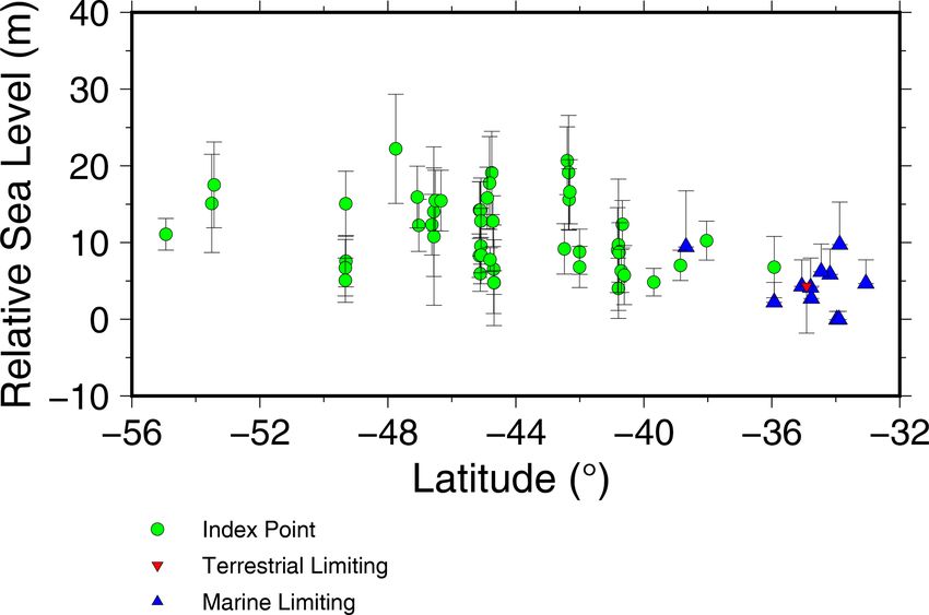
180                                                                            E. J. Gowan et al.: MIS 5e sea level in southeast South America

Table 7. Species of shells that have been dated in southeastern South America. Names are as reported in the original papers.

        Species                              Dating method              Locations
        Anomalocardia brasiliana             Radiocarbon                Puerto de Nueva Palmira
        Adelomelon ancilla                   AAR                        Caleta Valdés, San Antonio Oeste
        Amiantis purpurata                   AAR, ESR                   Caleta Olivia, San Antonio Oeste
        Aulacomya magellanica                AAR                        Puerto Deseado, San Antonio Oeste
        Brachidontes rodriguezi1             AAR                        Caleta Valdés, Puerto Deseado
        Buccinanops sp.                      AAR, radiocarbon           San Blas, Bahía Blanca
        Chione antigua                       Radiocarbon                Camarones
        Chione subrostrata                   Radiocarbon                Ezeiza
        Chlamys patriae                      AAR                        San Antonio Oeste
        Choromytilus sp.                     ESR                        San Blas
        Crepidula dilatata                   AAR                        San Antonio Oeste
        Erodona mactroides                   Radiocarbon                Southeast Entre Ríos Province, Martín García Island
        Glycymeris longior                   AAR, radiocarbon           San Antonio Oeste, Mar del Plata, Colorado River delta
        Glycymeris sp.                       AAR, U/Th                  Bahía Bustamante
        Macrocallista boliv.2                ESR, U/Th                  San Antonio Oeste
        Macrocallista sp.                    ESR, U/Th                  San Antonio Oeste
        Mactra sp.                           AAR                        Puente de Pascua
        Mactra isabelleana                   Radiocarbon                Puerto de Nueva Palmira, La Coronilla
        Mercenaria sp.                       ESR, U/Th                  Camarones, Caleta Olivia, Camarones
        Mytilus edulis                       AAR                        Caleta Valdés, San Antonio Oeste, San Blas
        Mytilus sp.                          ESR, U/Th                  Caleta Valdés, Mazarredo, San Julián
        Ostrea sp.                           Radiocarbon                Magdalena, Nicolás Vignogna III Quarry
        Ostrea equestris                     Radiocarbon                La Coronilla
        Patinigera magellanica               AAR                        Puerto Deseado
        Pelecypoda indet.                    ESR                        Caleta Valdés
        Perumytilus purpur3                  ESR                        Puerto Deseado
        Pitar rostrata                       AAR, ESR                   San Sebastián Bay, Caleta Valdés, San Antonio Oeste, San Blas
        Pitar sp.                            ESR, U/Th                  Caleta Valdés, Camerones, San Blas
        Protothaca ant.4                     AAR, ESR, U/Th             Bahía Bustamante, Caleta Olivia, Camarones, Mazarredo, Caleta Valdés
        Protothaca sp.                       AAR, ESR, U/Th             Bahía Bustamante, Caleta Olivia, Camarones, Mazarredo, San Julián
        Samarangia exalbida                  AAR                        San Antonio Oeste
        Tagelus gibbus                       Radiocarbon                Southeast Entre Ríos Province
        Tagelus sp.                          AAR                        Magdalena
        Tagelus plebeius                     Radiocarbon                Pilar, Zagarzazú
        Thais haemastoma                     Radiocarbon                Martín García Island
        Voluta sp.                           ESR, U/Th                  San Antonio Oeste
        Zidona angulata                      Radiocarbon                Colorado River delta
        Zidona dufresnei                     AAR                        Caleta Valdés, San Blas
      1 Standard spelling Brachidontes rodriguezii. 2 Full species name unknown. 3 Standard spelling Perumytilus purpuratus. 4 Full species name Protothaca antiqua.

shells. The result of these finite dates led some authors                                MIS 3 age became untenable (Rutter et al., 1989, 1990, 1992;
to suggest the possibility of an MIS 3 sea-level highstand                               Aguirre et al., 1995). Rojas and Martínez (2016) concluded
record along the Argentinian coast (Codignotto et al., 1988;                             that MIS 3-aged shells found in Uruguay Pleistocene de-
González et al., 1988b; González, 1992; Aguirre and What-                                posits were minimum ages, since the shell species were con-
ley, 1995). González and Guida (1990) supported this inter-                              sistent with warmer-than-present water temperatures, some-
pretation through the use of magnetostratigraphy and corre-                              thing that was unlikely to be true during the MIS 3 period.
lating reverse magnetized stratigraphic units to magnetic ex-                            Radiocarbon dating remains the most widely applied method
cursions (see Sect. 4.7). Cionchi (1987) and Radtke (1988)                               to date Holocene shorelines and has been successfully ap-
rejected the interpretation of the finite ages as reliable and                           plied to many of the same regions that have Pleistocene de-
suggested that they were contaminated with secondary car-                                posits (see Sect. 6.4).
bonates. With the introduction of other dating techniques ap-                               Radiocarbon dating of suspected Late Pleistocene mate-
plied to Argentinian coastal deposits, the assignment of an                              rial like shells requires careful pretreatment to remove sec-

Earth Syst. Sci. Data, 13, 171–197, 2021                                                                        https://doi.org/10.5194/essd-13-171-2021
E. J. Gowan et al.: MIS 5e sea level in southeast South America 181
ondary precipitates and other contaminants (Wood, 2015). MIS 5e (Mangerud et al., 1979). In Buenos Aires Province,
Techniques to produce reliable dates are reliant on acceler- the marine transgression correlated to MIS 5 is called the
ator mass spectrometry (AMS) radiocarbon measurements, Belgranense Stage (Aguirre and Whatley, 1995; Isla et al.,
so the conventional radiocarbon ages previously acquired in 2000; Martínez et al., 2016; Rojas and Martínez, 2016). At
South American deposits should be regarded, in the absence only one location identified in this review, Isla Navarino,
of further constraints, as minimum ages. However, we sug- Chile, is the age of the sea-level indicator constrained on
gest that minimum ages can still be used to distinguish be- the basis of its stratigraphic position below Wisconsin-aged
tween Holocene and Pleistocene deposits, the latter char- glacial sediments.
acterized by minimum radiocarbon ages. This is confirmed
by the fact that, in some places, Pleistocene deposits have 5 Relative sea-level indicators
been dated by both radiocarbon and other techniques (Rutter
et al., 1989, 1990; Aguirre et al., 1995; Rojas and Martínez, In total, we reviewed 60 documented possible MIS 5 sea-
2016). Marine deposits with minimum radiocarbon ages and level proxies, of which 48 are sea-level indicators, 11 are
at an adjacent elevation above the Holocene highstand posi- marine-limiting points, and 1 is terrestrial limiting. A plot
tion have been assigned to MIS 5 within WALIS. These data of the elevation of these proxies is presented in Fig. 10. Sea-
should be treated with caution and regarded as being of ex- level indicators have enough information to tie the feature
tremely poor quality. to sea level, while marine-limiting and terrestrial-limiting
points only have enough information to place the feature be-
4.7 Paleomagnetism low or above sea level, respectively. The paleo sea level is
calculated using the indicative range of the indicator, the re-
González and Guida (1990) reported paleomagnetic mea- ported elevation and thickness of the indicator, and the un-
surements as a way to distinguish between differently aged certainties applied to those measurements. The elevation of
Pleistocene shoreline deposits. In their paper, they reported sea-level indicators along the coast ranges between 0 and
reverse magnetized sediments, which they assigned MIS 3 30 m above mean sea level (a.m.s.l.). This large range reflects
and MIS 5 ages on the basis of correlation to magnetic ex- the uncertainty in elevation measurements; however, it could
cursions (i.e. geologically brief periods of a weak or reversed also reflect incorrect correlation to MIS 5e. There is also the
magnetic field). They regarded definitively reversed sedi- possibility that the elevation variability is a real feature re-
ments to be correlative to the Blake Excursion. The Blake lated to glacial isostatic processes (see Sect. 6.5.2). The lo-
Excursion happened during MIS 5d, between 112–116 ka cations in this section are described in order of north to south
(Rossi et al., 2014). Since the MIS 5 highstand more likely along the southeastern South American coast.
happened during MIS 5e and MIS 5d sea level was tens of
meters below the present sea level (Lambeck and Chappell,
2001), either the magnetic measurements are in error or the 5.1 Uruguay
deposit is not MIS 5e in age. González and Guida (1990) in- Uruguay has data at three locations (Fig. 6).
terpreted some deposits with anomalous magnetism that also
had finite radiocarbon ages as being correlative to the Lake
5.1.1 La Coronilla
Mungo excursion. The Lake Mungo excursion was reported
to have happened at about 30 ka, but recently this has been Martínez et al. (2001), Rojas and Martínez (2016), and Ro-
discredited (Roberts, 2008). We put no confidence in the abil- jas et al. (2018a) describe a 0.6 m thick marine deposit with
ity of these measurements to assign an age to the deposits and abundant marine mollusc fossils located at the modern coast.
do not use them to assign an MIS 5 age. They interpreted the deposit to represent a low-energy envi-
ronment, such as a bay. The age of the deposit is only con-
4.8 Stratigraphy strained with minimum-age radiocarbon dates. A taxonomic
analysis by Rojas et al. (2018b) identified many species that
South American geologists who have worked on paleo sea are currently found 600 km north of La Coronilla, indicat-
level have tended to use the glacial–interglacial chronostrati- ing warmer-than-present water conditions, which they inter-
graphic nomenclature used in North America. The Wisconsin preted as supporting an MIS 5e age assignment. The marine-
glaciation represents the most recent glacial period, covering limiting elevation is 0.50 ± 0.53 m.
MIS 5d-2 (Otvos, 2015). The Sangamon interglacial repre-
sents the last interglacial, broadly defined as the period when
5.1.2 Zagarzazú
there were dominantly non-glacial conditions in the Ameri-
cas. Some definitions place the Sangamonian to encompass Rojas and Martínez (2016) and Rojas et al. (2018a) described
all of MIS 5, but more recent definitions narrow it to only a thin (0.5 m) exposure of marine sediments at the modern
MIS 5e (Otvos, 2015). It is therefore roughly equivalent to coast containing shells in living position. A radiocarbon date
the European Eemian Stage, which strictly correlates with from this site yielded a minimum-limiting date, while an
https://doi.org/10.5194/essd-13-171-2021 Earth Syst. Sci. Data, 13, 171–197, 2021182 E. J. Gowan et al.: MIS 5e sea level in southeast South America
Figure 6. MIS 5 sea-level indicators in Uruguay (black circles).
OSL date supports an MIS 5a age assignment. The marine-
limiting elevation is 0.50 ± 0.53 m. An analysis of the fossil
shell species indicated that conditions were more saline than
at present, but since there were fewer warm-water species
than in the La Coronilla section, they concluded an MIS 5a
age was more likely (Rojas and Martínez, 2016).
5.1.3 Puerto de Nueva Palmira
Marine deposits, interpreted as having been deposited in a
proximal, wave-dominated environment, at Puerto de Nueva
Palmira were described by Martínez et al. (2001), Rojas
and Martínez (2016), and Rojas et al. (2018a). The de-
posit (about 1.5 m thick) contained disarticulated, randomly
oriented shell fossils. Martínez et al. (2001) collected two
minimum-age radiocarbon dates from this deposit but in-
terpreted the deposit as being from the last interglacial on
the basis of marine fauna indicating a relatively warm envi-
ronment. Rojas and Martínez (2016) reported an OSL date
of 80.7 ± 5.5 ka, which suggests an MIS 5a assignment, but
they were cautious about assigning a specific substage of
MIS 5 to the deposit. From faunal analysis, they suggested
that the environment was not necessarily warmer, as the La
Coronilla assemblage suggests. This means an MIS 5a as-
signment is plausible. This deposit gives a marine-limiting
elevation of 12.5 ± 2.8 m.
5.2 Northern Argentina – Entre Ríos and Buenos Aires
provinces
Entre Ríos Province and Buenos Aires Province have data at
14 locations (Fig. 7).
5.2.1 Southeast Entre Ríos Province Figure 7. MIS 5 sea-level indicators in Entre Ríos and Buenos
González et al. (1986, 1988b) and González and Guida Aires provinces, Argentina (black circles).
(1990) describe a Pleistocene estuary deposit in a location
called Irazusta Quarry. The exact location is estimated based
Earth Syst. Sci. Data, 13, 171–197, 2021 https://doi.org/10.5194/essd-13-171-2021E. J. Gowan et al.: MIS 5e sea level in southeast South America 183
on a map from the paper but is likely over 100 km from the The lowest facies was interpreted as a salt marsh; the sec-
modern coast. The deposit was about 1.2 m thick and con- ond facies was deposited in a coastal creek environment, and
tained shells that indicate a brackish environment, overlying the upper facies is composed of beach-like deposits associ-
a relic shore platform. They collected three finite radiocarbon ated with storm surges. In the present day, storm surges that
dates, but these are regarded as minimum ages. The mini- form these kind of deposits reach between 1 and 4.4 m above
mum sea level from this deposit is 6.2 ± 1.5 m. We applied present sea level. The environmental conditions derived from
an uncertainty from the modern tidal range using the near- fossils in the deposit indicate a range of conditions, from
est tide gauge, on Martín García Island. Based on the simi- freshwater to marine, so we interpret this as being terrestrial
larity in elevation of this deposit to the Magdalena site (see limiting (i.e. forming above mean sea level but influenced
Sect. 5.2.7), we infer it is MIS 5 in age. by seawater at least periodically). Gasparini et al. (2016) re-
González et al. (1988b) and González and Guida (1990) ported a radiocarbon date from the beach-like deposit and,
completed magnetostratigraphic analysis of the substrate due to the sedimentary environment, considered it to be ter-
upon which the platform surface was formed, a lagoon de- restrial limiting. An OSL date from the beach-like deposit
posit. The reverse polarity of the sediments prompted cor- gave a date of 60 ka (Beilinson et al., 2019), which also likely
relation of the lagoon deposit with the Blake Excursion, a underestimates the true age. If this deposit formed during
minor reversal during MIS 5d. However, due to the impli- MIS 5, it gives a terrestrial-limiting elevation of 1.3 ± 3.1 m.
cations for the necessary uplift to place MIS 5d sediments
above modern sea level (see Sect. 4.7), this correlation is con- 5.2.6 Hudson
sidered to be incorrect.
Zárate et al. (2009) described a section located at Hudson
5.2.2 Martín García Island
(Fig. 7). Within the section was a laterally discontinuous ma-
rine clayey silt, interpreted as being deposited in a distal tidal
González and Ravizza (1987) and González et al. (1986) de- channel, with marine fossils. OSL dating of this unit is con-
scribe a thin (0.4 m) Pleistocene estuary deposit adjacent to a sistent with an MIS 5 age assignment. The marine-limiting
paleo-cliff on Martín García Island. Based on finite radiocar- elevation is 6.1 ± 1.9 m.
bon ages, they assigned an MIS 3 age; we regard this as an
minimum age. Based on similar elevation and stratigraphy to 5.2.7 Magdalena
the Magdalena site (Sect. 5.2.7), we regard this deposit to be
MIS 5 in age. The marine-limiting elevation from this deposit Weiler et al. (1988) and González et al. (1986) describe
is 7.5 ± 1.7 m. a thin (0.2 m) estuary deposit beneath a paleo-cliff deposit
at Cañada de Arregui, near Magdalena. Radiocarbon ages
5.2.3 Pilar
from this deposit gave minimum ages (Aguirre et al., 1995).
Aguirre and Whatley (1995) and Aguirre et al. (1995) col-
Fucks et al. (2005) describe a Pleistocene-aged estuary de- lected Tagelus sp. mollusc shells for AAR analysis from
posit, with a maximum elevation of 8 m. A radiocarbon-dated the same outcrop. The AAR values for the outcrop were
shell returned an infinite age. If this deposit is MIS 5 in age, higher than Holocene samples from the same location. Us-
it has a marine-limiting elevation of 8 ± 1.8 m. Based on the ing the Holocene data for calibration, a numerical age dating
similarity in elevation to the Magdalena site (Sect. 5.2.7), we to 106 ka was determined, which is consistent with an MIS 5
regard this as an MIS 5 deposit. age. The minimum sea level from this deposit is 6.0 ± 1.7 m.
Although this site has relatively good age control, the lack
5.2.4 Ezeiza
of information on elevation measurements means that it is
relatively low quality.
Martínez et al. (2016) investigated mollusc fauna from ma-
rine sediments exposed at a riverbank in Ezeiza. Two radio- 5.2.8 Puente de Pascua
carbon dates from the deposit gave minimum-limiting dates.
The species found in the sediment indicate warmer-than- Aguirre and Whatley (1995) and Aguirre et al. (1995) col-
present water conditions, which led them to conclude the sed- lected Tagelus mollusc shell samples for AAR dating from a
iment corresponds to MIS 5e. The marine-limiting elevation well-cemented coquina at Puente de Pascua. An AAR date of
is 3.5 ± 0.8 m. 123 ka is consistent with an MIS 5 deposit. However, insuffi-
cient information is given to ascertain an indicative meaning,
5.2.5 Nicolás Vignogna III Quarry
so we assign this data point as marine limiting, with an ele-
vation of 3.5 ± 1.3 m.
Beilinson et al. (2019) described a sedimentary sequence in Fucks et al. (2006, 2010) returned to this location and un-
a quarry southwest of Buenos Aires (Fig. 7). There were dertook a further investigation of the MIS 5 deposit. They
three facies they interpreted as being associated with MIS 5. reported a 0.7 m thick sand deposit with lenses of shells that
https://doi.org/10.5194/essd-13-171-2021 Earth Syst. Sci. Data, 13, 171–197, 2021184 E. J. Gowan et al.: MIS 5e sea level in southeast South America
they interpreted to be a beach deposit. The reported elevation 5.2.13 Bahía Anegada
of the deposit (6–8 m) is higher than that reported by Aguirre
and Whatley (1995) and Aguirre et al. (1995) (3–4 m). The Weiler (1993) described several individual pre-Holocene
calculated sea level from this deposit is 6.8 ± 4.0 m. beach ridge deposits in Bahía Anegada. These deposits had
minimum radiocarbon ages. Unfortunately, elevation mea-
surements are not available, and this location was not added
5.2.9 Mar del Plata
to the database.
González et al. (1986) gave a brief description of a trans- Fucks et al. (2012a) revisited the sites and reported eleva-
gressive beach deposit. Radiocarbon dating provided mini- tions of 8–10 m, which was possibly based off values from
mum ages. A magnetostratigraphic analysis of this deposit topographic maps or Google Earth. They correlated them to
showed that it has negative magnetic polarity. González and MIS 5 on the basis of similar elevation to other dated land-
Guida (1990) interpreted this to be correlative to the Lake forms in the region. However, there is not a sufficient de-
Mungo magnetic excursion, which they correlated to MIS 3 scription of the deposits or of dating to include them in our
on the basis of the radiocarbon dates (which they regarded database. Charó et al. (2013a) further analyzed the faunal
as reliable). We have included this point as an MIS 5 deposit content and found a higher abundance of species in the de-
based on elevation. Though if the magnetic measurements posits attributed to MIS 5e, which they interpreted to indicate
are reliable, this would indicate that an MIS 5e age assign- warmer water conditions.
ment is unlikely. The calculated sea level from this deposit is
10.3 ± 2.5 m.
5.2.14 San Blas
5.2.10 Claromecó
Trebino (1987) described the geomorphology and raised
Isla et al. (2000) and Isla and Angulo (2016) reported on a
shorelines in the San Blas area. They described two groups
beach deposit that was assigned to MIS 5 using a U/Th date.
of shorelines: one that was Holocene in age and another that
The calculated sea level from this deposit is 7.0 ± 2.0 m.
was determined to be Pleistocene on the basis of finite ra-
diocarbon dates. The Pleistocene group, at a higher eleva-
5.2.11 Bahía Blanca tion, consists of three beach ridges with elevations of 9–
González et al. (1986, 1988b) described an estuary deposit, 10 m. We correlate the shorelines to MIS 5, with low con-
overlying a cemented delta deposit. The estuary deposit fidence. Trebino (1987) reported that the modern elevation
contained many mollusc fossils that had minimum radio- range for coastal dune and beach deposits is between 0.5 and
carbon ages. The minimum sea level from this deposit is 7 m, which we take as the modern analogue. We calculate a
13.5 ± 3.6 m. The relatively high elevation of this deposit paleo sea level of 5.8 ± 3.8 m from these shorelines.
and the Holocene highstand deposits (> 10 m a.m.s.l.) led Rutter et al. (1989) collected fossil mollusc shells at two
González et al. (1988b) to hypothesize that this location is sites in San Blas, both of which were interpreted as being
uplifting. Aliotta et al. (2001) investigated these deposits and Pleistocene in age on the basis of AAR values. The sam-
concluded that the depositional environment during the Pleis- ples were taken from a 1.2 m thick beach deposit (SB-2) and
tocene was lower energy than that during the Holocene high- a 6 m thick beach gravel layer within a 10 m high section
stand. (SB-1). When comparing the same species, the AAR values
were generally lower for the samples taken at SB-2 than for
those taken at SB-1, which implies the SB-1 site represents
5.2.12 Colorado River delta
an older deposit. Rutter et al. (1989) defined the SB-2 deposit
González et al. (1986, 1988b) briefly described a beach ridge as an “intermediate”-aged deposit, older than Holocene, and
deposit with fossil mollusc shells that had minimum radio- cautiously assigned an MIS 5 age. The calculated sea level
carbon ages. The calculated sea level from this deposit is of SB-2 is 12.4 ± 3.1 m. ESR dating of mollusc shells from
4.8 ± 1.8 m. Fucks et al. (2012a) also mapped Pleistocene the deposit at SB-1 returned ages that were consistent with
marine deposits that they correlated to MIS 5 in the Colorado an MIS 5 age (Rutter et al., 1990), which contradicts the au-
River region, but there is not enough information for an as- thors’ earlier interpretation that the deposit is significantly
sessment of paleo sea level. Charó et al. (2015) investigated older. If accepted as being MIS 5, the calculated sea level is
the faunal composition at sites they interpreted to be MIS 5e 4.0 ± 3.9 m. Fucks et al. (2012a) also investigated this loca-
and found the faunal content was similar to that of Holocene tion and reported on mollusc species. Charó et al. (2013b)
deposits. Since they did not present any numerical dating, compared the faunal content of shoreline deposits attributed
there is not enough information to include these sites in the to MIS 5e and the Holocene in the San Blas area. Due to
database. the presence of Crassostrea rhizophorae, they interpreted the
conditions to be warmer in the MIS 5e deposits, although
overall, the species content was similar. Since these deposits
Earth Syst. Sci. Data, 13, 171–197, 2021 https://doi.org/10.5194/essd-13-171-2021You can also read