CALIBRATION OF A 35 GHZ AIRBORNE CLOUD RADAR: LESSONS LEARNED AND INTERCOMPARISONS WITH 94 GHZ CLOUD RADARS - MPG.PURE
←
→
Page content transcription
If your browser does not render page correctly, please read the page content below
Atmos. Meas. Tech., 12, 1815–1839, 2019
https://doi.org/10.5194/amt-12-1815-2019
© Author(s) 2019. This work is distributed under
the Creative Commons Attribution 4.0 License.
Calibration of a 35 GHz airborne cloud radar: lessons learned and
intercomparisons with 94 GHz cloud radars
Florian Ewald1 , Silke Groß1 , Martin Hagen1 , Lutz Hirsch2 , Julien Delanoë3 , and Matthias Bauer-Pfundstein4
1 DeutschesZentrum für Luft- und Raumfahrt, Institut für Physik der Atmosphäre, Oberpfaffenhofen, Germany
2 Max Planck Institute for Meteorology, Hamburg, Germany
3 LATMOS/UVSQ/IPSL/CNRS, Guyancourt, France
4 Metek GmbH, Elmshorn, Germany
Correspondence: Florian Ewald (florian.ewald@dlr.de)
Received: 17 August 2018 – Discussion started: 11 October 2018
Revised: 8 February 2019 – Accepted: 14 February 2019 – Published: 20 March 2019
Abstract. This study gives a summary of lessons learned measured during previous campaigns had to be corrected by
during the absolute calibration of the airborne, high-power +7.6 dB.
Ka-band cloud radar HAMP MIRA on board the German re- To validate this internal calibration, the well-defined ocean
search aircraft HALO. The first part covers the internal cali- surface backscatter was used as a calibration reference. With
bration of the instrument where individual instrument com- the new absolute calibration, the ocean surface backscatter
ponents are characterized in the laboratory. In the second measured by HAMP MIRA agrees very well (< 1 dB) with
part, the internal calibration is validated with external refer- modeled values and values measured by the GPM satellite.
ence sources like the ocean surface backscatter and different As a further cross-check, flight experiments over Europe and
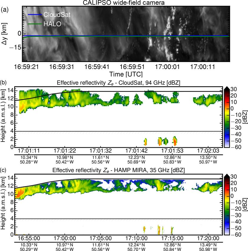
air- and spaceborne cloud radar instruments. the tropical North Atlantic were conducted. To that end, a
A key component of this work was the characterization joint flight of HALO and the French Falcon 20 aircraft, which
of the spectral response and the transfer function of the re- was equipped with the RASTA cloud radar at 94 GHz and
ceiver. In a wide dynamic range of 70 dB, the receiver re- an underflight of the spaceborne CloudSat at 94 GHz were
sponse turned out to be very linear (residual 0.05 dB). Using performed. The intercomparison revealed lower reflectivi-
different attenuator settings, it covers a wide input range from ties (−1.4 dB) for RASTA but slightly higher reflectivities
−105 to −5 dBm. This characterization gave valuable new (+1.0 dB) for CloudSat. With effective reflectivities between
insights into the receiver sensitivity and additional attenua- RASTA and CloudSat and the good agreement with GPM,
tions which led to a major improvement of the absolute cali- the accuracy of the absolute calibration is estimated to be
bration. The comparison of the measured and the previously around 1 dB.
estimated total receiver noise power (−95.3 vs. −98.2 dBm)
revealed an underestimation of 2.9 dB. This underestimation
could be traced back to a larger receiver noise bandwidth
of 7.5 MHz (instead of 5 MHz) and a slightly higher noise 1 Introduction
figure (1.1 dB). Measurements confirmed the previously as-
sumed antenna gain (50.0 dBi) with no obvious asymmetries In recent years, the deployment of cloud profiling microwave
or increased side lobes. The calibration used for previous radars on the ground, on aircraft as well as on satellites,
campaigns, however, did not account for a 1.5 dB two-way like CloudSat (Stephens et al., 2002) or the upcoming Earth-
attenuation by additional waveguides in the airplane instal- CARE satellite mission (Illingworth et al., 2014), have
lation. Laboratory measurements also revealed a 2 dB higher greatly advanced our scientific knowledge of cloud micro-
two-way attenuation by the belly pod caused by small devi- physics. Nevertheless, large discrepancies in retrieved cloud
ations during manufacturing. In total, effective reflectivities microphysics (Zhao et al., 2012; Stubenrauch et al., 2013)
contribute to uncertainties in the understanding of the role of
Published by Copernicus Publications on behalf of the European Geosciences Union.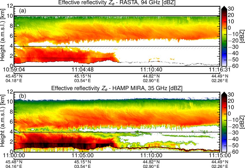
1816                                                                F. Ewald et al.: Calibration of a 35 GHz airborne cloud radar

clouds for the climate system (Boucher et al., 2013). An im-            surface backscatter (Durden et al., 1994; Z. Li et al., 2005;
portant aspect for enabling accurate microphysical retrievals           Tanelli et al., 2006). For this incidence angle, these studies
based on cloud radar data is the proper calibration of the sys-         confirmed the ocean surface to be relatively insensitive to
tems.                                                                   changes in wind speed and wind direction.
   However, the absolute calibration of an airborne                        Subsequent studies followed suit, applying the same tech-
millimeter-wave cloud radar can be a challenging task.                  nique to other airborne cloud radar instruments: the Japanese
Its initial calibration demands detailed knowledge of cloud             W-band Super Polarimetric Ice Crystal Detection and Expli-
radar technology and the availability of suitable mea-                  cation Radar (SPIDER; Horie et al., 2000) on board the NICT
surement devices. During cloud radar operation, system                  Gulfstream II by Horie et al. (2004), the Ku/Ka-band Air-
parameters of transmitter and receiver system can drift due             borne Second Generation Precipitation Radar (APR-2; Sad-
to changing ambient temperature, pressure and aging system              owy et al., 2003) on board the NASA P-3 aircraft by Tanelli
components. The validation of the absolute calibration with             et al. (2006) and the W-band cloud radar (RASTA; Protat
external sources is furthermore complicated for downward-               et al., 2004) on board the SAFIRE Falcon 20 by Bouniol et al.
looking installations on an aircraft. The missing ability of            (2008).
most airborne and many ground-based radars to point their                  Encouraged by these airborne studies, this in-flight cali-
line of sight to an external reference source makes it difficult        bration technique has also been proposed and successfully
or even completely impossible to calibrate the overall system           applied to the spaceborne CloudSat instrument (Stephens
with an external reference in a laboratory.                             et al., 2002; Tanelli et al., 2008). Based on this success, Horie
   Typically, an budget approach is used for the absolute cal-          and Takahashi (2010) proposed the same technique with a
ibration of airborne cloud radar instruments. First, the instru-        whole 10◦ across-track sweep for the next spaceborne cloud
ment components like transmitter, receiver, waveguides, an-             radar, the 94 GHz Doppler Cloud Profiling Radar (CPR) on
tenna and radome are characterized individually in the lab-             board EarthCARE (Illingworth et al., 2014).
oratory. During in-flight measurements, variable component                 With CloudSat as a long-term cloud radar in space, direct
parameters are then monitored and corrected for drifts using            comparisons of radar reflectivity from ground- and airborne
the laboratory characterization. Subsequently, all gains and            instruments became possible (Bouniol et al., 2008; Protat
losses are combined into an overall instrument calibration.             et al., 2009). While the first studies still assessed the stability
   In order to meet the required absolute accuracy and to               of the spaceborne instrument, subsequent studies turned this
follow good scientific practice, an external in-flight calibra-         around by using CloudSat as a Global Radar Calibrator for
tion becomes indispensable to check the internal calibration            ground-based or airborne radars Protat et al. (2010).
for systematic errors. For weather radars, the well-defined                This work will focus on the internal and external cali-
reflectivity of calibration spheres on tethered balloons or             bration of the MIRA cloud radar (Mech et al., 2014) on
erected trihedral corner reflectors has been a reliable exter-          board the German High Altitude and Long Range Research
nal reference for years (Atlas, 2002). In more recent years,            Aircraft (HALO), adopting the ocean surface backscattering
this technique is being extended to scanning, ground-based              technique described by Z. Li et al. (2005). In the first part,
millimeter-wave radars (Vega et al., 2012; Chandrasekar                 the preflight laboratory characterization of each system com-
et al., 2015). For the airborne perspective on the other hand,          ponent will be described. This includes antenna gain, com-
the direct fly-over and the subsequent removal of additional            ponent attenuation and receiver sensitivity. In a budget ap-
background clutter is difficult to reproduce (Z. Li et al.,             proach, these system parameters are then used in combina-
2005).                                                                  tion with in-flight monitored transmission and receiver noise
   Driven by this challenge, many studies have been con-                power levels to form the internal calibration. The second part
ducted to characterize the characteristic reflectivity of the           will then compare the internal calibration with external ref-
ocean surface using microwave scatterometer–radiometer                  erence sources in-flight. As external reference sources, mea-
systems in the X and Ka bands (Valenzuela, 1978; Masuko                 surements of the ocean surface as well as intercomparisons
et al., 1986). As one of the first, Caylor (1994) introduced the        with other air- and spaceborne cloud radar instruments will
ocean surface backscatter technique to cross-check the in-              be used.
ternal calibration of the NASA ER-2 Doppler radar (EDOP;                   This paper is organized as follows: after some considera-
Heymsfield et al., 1996). In an important next step, L. Li et al.       tions about required radar accuracies shown in Sect. 1, Sect. 2
(2005) combined this technique with analytical models of                introduces the cloud radar instrument and its specifications
the ocean surface backscatter. In their work, they used circle          on board the HALO research aircraft. Section 3 recalls the
and roll maneuvers to sample the ocean surface backscatter              radar equation and introduces the concept of using the ocean
for different incidence angles with the Cloud Radar System              surface backscatter for radar calibration. The characteriza-
(CRS; Li et al., 2004), a 94 GHz (W band) cloud radar on                tion and calibration of the single system components, in-
board the NASA ER-2 high-altitude aircraft. In this context,            cluding waveguides, antenna and belly pod, is described in
they proposed to point the instrument 10◦ off-nadir, an an-             Sect. 3.1. Subsequently, the overall calibration of the radar
gle for which multiple studies found a very constant ocean              receiver is explained in Sect. 3.2. Here, a central innovation

Atmos. Meas. Tech., 12, 1815–1839, 2019                                                    www.atmos-meas-tech.net/12/1815/2019/
F. Ewald et al.: Calibration of a 35 GHz airborne cloud radar                                                                    1817

of this work is the determination of the receiver sensitivity
(Sect. 3.3 and 3.4). In the second part of the paper, the bud-
get calibration is validated by using predicted and measured
ocean surface backscatter (Sect. 4.3). In addition, the calibra-
tion and system performance for joint flight legs is compared
to the W-band cloud radars like the airborne cloud radar
RASTA (Sect. 5.2) and the spaceborne cloud radar CloudSat
(Sect. 5.3).

Accuracy considerations

In order to provide scientifically sound interpretations of
cloud radar measurements, a well-calibrated instrument with
known sensitivity is indispensable. Many spaceborne (De-           Figure 1. Microphysical retrieval uncertainty due to different abso-
lanoë and Hogan, 2008; Deng et al., 2010) or ground-based          lute calibration uncertainties (±1, ±3, ±8) for mono-disperse cloud
(Donovan et al., 2000) techniques to retrieve cloud micro-         water droplets according to Mie calculations.
physics using millimeter-wave radar measurements require
a well-calibrated instrument. In the case of the CloudSat
instrument, the calibration uncertainty was specified to be        of an offset in radar reflectivity when comparing different
±2 dB or better (Stephens et al., 2002). This requirement for      cloud radar instruments. In a direct comparison with the W-
absolute calibration imposed by retrievals of cloud micro-         Band (94 GHz) ARM Cloud Radar (WACR), Handwerker
physics is further explained in Fig. 1. Under the simplest as-     and Miller (2008) found reflectivities around 3 dB smaller
sumption of small, mono-disperse cloud water droplets, the         for the Karlsruhe Institute of Technology MIRA, contradict-
iso-lines in Fig. 1 represent all combinations of cloud droplet    ing the reflectivity-reducing effect of a higher gaseous atten-
effective radius and liquid water content with a radar reflec-     uation and stronger Mie scattering at 94 GHz. Protat et al.
tivity of −20 dBz. An increasing retrieval ambiguity, caused       (2009) could reproduce this discrepancy in a comparison
by an assumed instrument calibration uncertainty, is illus-        with CloudSat, where they found a clear systematic shift of
trated by the shaded areas with ±1 dB (green), ±3 dB (yel-         the mean vertical profile by 2 dB between Cloudsat and the
low) and ±8 dB (red). To constrain the retrieval space consid-     Lindenberg MIRA (CloudSat showing higher values than the
erably within synergistic radar–lidar retrievals like Cloudnet     Lindenberg radar).
(Illingworth et al., 2007) or Varcloud (Delanoë and Hogan,
2008), the absolute calibration uncertainty has to be signif-
icantly smaller than the natural variability of clouds. Since      2   The 35 GHz cloud radar on HALO
a reflectivity bias of 8 dB would bias the droplet size by a
factor of 2 and the water content by even an order of mag-         The cloud radar on HALO is a pulsed Ka-band, polarimetric
nitude, the absolute calibration uncertainty should be at least    Doppler millimeter-wavelength radar which is based on pro-
3 dB or lower. For a systematic 1 dB calibration offset, Pro-      totypes developed and described by Bormotov et al. (2000)
tat et al. (2016) still found ice water content biases of +19 %    and Vavriv et al. (2004). The current system was manufac-
and −16 % in their radar-only retrieval. Since HAMP MIRA           tured and provided by Metek (Meteorologische Messtech-
data are used in retrievals of cloud microphysics, the target      nik GmbH, Elmshorn, Germany). The system design and
accuracy will be set to 1 dB.                                      its data processing, including an updated moment estimation
   An accurate absolute calibration is further motivated by        and a target classification by Bauer-Pfundstein and Görsdorf
recent studies (Protat et al., 2009; Hennemuth et al., 2008;       (2007), was described in detail by Görsdorf et al. (2015). The
Maahn and Kollias, 2012; Ewald et al., 2015; Lonitz et al.,        millimeter radar is part of the HALO Microwave Package
2015; Myagkov et al., 2016; Acquistapace et al., 2017),            (HAMP) which will be subsequently abbreviated as HAMP
which used the radar reflectivity provided by almost identi-       MIRA. Its standard installation in the belly pod section of
cal ground-based versions of the same instrument. The in-          HALO with its fixed nadir-pointing 1 m diameter Cassegrain
stallation of the MIRA instrument on many ground-based             antenna is described in detail by Mech et al. (2014). Its trans-
cloud profiling sites within ACTRIS (Aerosols, Clouds and          mitter is a high-power magnetron operating at 35.5 GHz with
Trace gases Research InfraStructure Network; http://www.           a peak power Pt of 27 kW, with a pulse repetition frequency
actris.eu, last access: 10 March 2019) and in the framework        fp between 5 and 10 kHz and a pulse width τp between 100
of Cloudnet is a further incentive for an external calibration     and 400 ns. The large antenna and the high peak power can
study.                                                             yield an exceptionally good sensitivity of −47 dBZ for the
   The need for an external calibration is furthermore en-         ground-based operation (5 km distance, 1 s averaging and a
couraged by several studies which already found evidence           range resolution of 30 m). In the current airborne configu-

www.atmos-meas-tech.net/12/1815/2019/                                                 Atmos. Meas. Tech., 12, 1815–1839, 2019
1818 F. Ewald et al.: Calibration of a 35 GHz airborne cloud radar
Table 1. Technical specifications of the HAMP cloud radar as char- constant Rc contains the pulse wavelength λ (m), pulse width
acterized in this work. Boldface indicates the operational configu- τp (s) and peak transmit power Pt in milliwatts, the peak an-
ration used in this work. tenna gain Ga , and the antenna half-power beamwidth φ.
Additionally, it accounts for all attenuations Lsys occurring
Parameter Variable Value in system components, e.g., in transmitter (Ltx ) and receiver
Wavelength λ 8.45 mm (Lrx ) waveguides, due to the belly pod radome L2bp and due
Pulse power Pt 27 kW to the finite receiver bandwidth (Lfb ):
Pulse repetition fp 5–10 kHz
Pulse width τp 100, 200, 400 ns 1024 ln 2λ2 1018 Lsys
Receive window τr 100, 200, 400 ns Rc = . (3)
Pt G2a cτp π 3 φ 2 |K|2
RF noise bandwidth Bn 7.5, 5 MHz
RF front-end noise figure NF 9.9 dB Usually, antenna parameters (Ga , φ) and system losses
RF front-end sensitivity Pn −95.3 dBm
(Lsys = Ltx L2bp Lrx ) have to be determined only once for
Sensitivitya (ground) Zmin −47.5 dBZ
Sensitivitya (airborne) Zmin −39.8 dBZ
each system modification. In contrast, transmitter and re-
Antenna gain Ga 50.0 dB ceiver parameters have to be monitored continuously. In ad-
Beamwidth (3 dB) φ 0.56◦ dition, a thorough characterization of the receiver sensitivity
Atten. (finite bandwidth) Lfb 1.2 dB is essential for the absolute accuracy of the instrument.
Atten. (Tx path) Lrx 0.75 dB
Atten. (Rx path) Ltx 0.75 dB
Atten. (belly pod) Lbp 1.5 dB 3 Internal calibration
a At 5 km, 1 s average, 30 m resolution.
This section will discuss the internal calibration of the radar
instrument and its characterization in the laboratory. The fol-
lowing section will then compare this budget approach in-
ration, the sensitivity is reduced to −39.8 dBZ by various flight with an external reference source.
circumstances which will be addressed in this paper. The The monitoring of the system-specific parameters and the
broadening of the Doppler spectrum due to the beam width subsequent estimation of effective reflectivity are described
can reduce this sensitivity further by 9 dB, as discussed in in detail by Görsdorf et al. (2015). The internal calibration
Mech et al. (2014). Table 1 lists the technical specifications (budget calibration) strategy for HAMP MIRA is therefore
as characterized in this work. Boldface indicates the opera- only briefly summarized here. In case of a deviation, pre-
tional configuration. viously assumed and used parameters will be given and re-
Most of the parameters in Table 1 play a role in the abso- ferred to as initial calibration for traceability of past radar
lute calibration of the cloud radar instrument. For this reason, measurements.
this section will briefly recapitulate the conversion from re-
ceiver signal power to the commonly used equivalent radar 3.1 Antenna, radome and waveguides
reflectivity factor Ze . When the radar reflectivity η of a tar-
get is known, e.g., in modeling studies, its equivalent radar – Antenna. The gain Ga = 50.0 dBi and the beam pat-
reflectivity factor is given by tern (−3 dB beamwidth φ = 0.56◦ ) was determined by
the manufacturer following the procedure described
ηλ4 by Myagkov et al. (2015). Hereby the 1 m diameter
Ze = , (1)
|K|2 π 5 Cassegrain antenna was installed on a pedestal to scan
its pattern on a tower 400 m away. The antenna pattern
where |K|2 = 0.93 is the dielectric factor for water and λ the showed no obvious asymmetries or increased side lobes
radar wavelength. For brevity, the equivalent radar reflectiv- (side lobe level: −22 dB). Its characterization revealed
ity factor Ze is referred to as “effective reflectivity” in this no significant differences in comparison with the ini-
paper. Following the derivation of the meteorological form tially estimated parameters (Ga = 49.75 dBi, φ = 0.6◦ ).
of the radar equation by Doviak and Zrnić (2006), the ef-
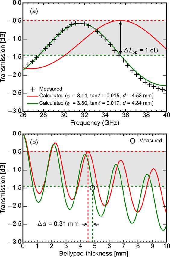
fective reflectivity Ze (mm6 m−3 ) can be calculated from the – Radome. The thickness of the epoxy quartz radome in
received signal power Pr (W) by the belly pod was designed with a thickness of 4.53 mm
to limit the one-way attenuation to around 0.5 dB. Devi-
Ze = Rc Pr r 2 L2atm , (2) ations during manufacturing increased the thickness to
4.84 mm, with a one-way attenuation of around 1.5 dB.
where r is the range between antenna and target, Latm is the Laboratory measurements confirmed this 2.0 dB (2 ×
one-way path integrated attenuation, and Rc is a constant 1.0 dB) higher two-way attenuation compared to the ini-
which describes all relevant system parameters. Assuming tially used value for the radome attenuation. A detailed
a circularly symmetric Gaussian antenna pattern, this radar analysis of this deviation can be found in Appendix B.
Atmos. Meas. Tech., 12, 1815–1839, 2019 www.atmos-meas-tech.net/12/1815/2019/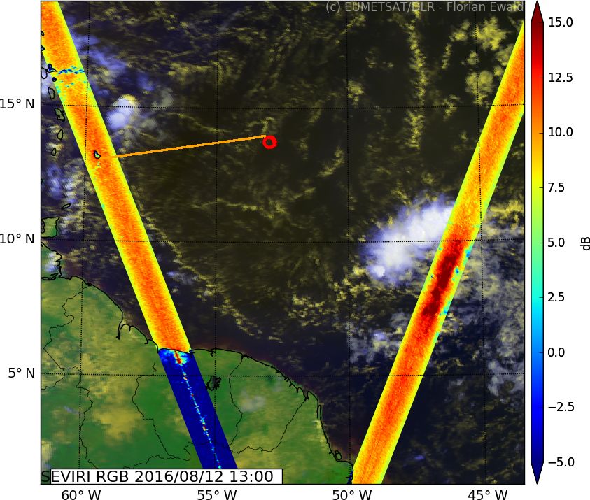
F. Ewald et al.: Calibration of a 35 GHz airborne cloud radar                                                                1819

  – Waveguides. The initially used calibration did not ac-             To obtain the received backscattered signal Sr in atmo-
    count for the losses caused by the longer waveguides               spheric gates, one has to subtract the signal received in
    in the airplane installation. Actually, transmitter and re-        the noise gate Sng from the total received signal S since
    ceiver waveguides each have a length of 1.15 m. With               it contains both signal and noise:
    a specified attenuation of 0.65 dB m−1 , the two-way at-
    tenuation by waveguides is thus 1.5 dB.                            Sr = S − Sng .                                          (7)

3.2   Transmitted and received signal power                            In that way, a signal-to-noise ratio is then calculated by
                                                                       dividing the received backscattered signal Sr in each at-
  – Transmitter peak power Pt . Due to strong variations               mospheric gate by the signal Sng measured in the noise
    in ambient temperatures in the cabin, in-flight thermis-           gate:
    tor measurements proved to be unreliable. For this rea-
                                                                                 Sr
    son, thermally controlled measurements of Pt were con-             SNR† =        .                                         (8)
    ducted on the ground, which were correlated with mea-                        Sng
    sured magnetron currents Im . The relationship between             The relative power of the calibration gate to the re-
    both parameters then allowed Pt to be derived from in-             ceiver noise gate is furthermore used to monitor the re-
    flight measurements of Im . A detailed analysis of this            ceiver sensitivity (for details see Sect. 3.3). The main
    relationship can be found in Appendix A.                           advantage of this method is the simultaneous monitor-
  – Finite receiver bandwidth loss Lfb . The loss caused by            ing of the relative receiver sensitivity using the same cir-
    a finite receiver bandwidth was discussed in detail by             cuitry that is used for atmospheric measurements. Fur-
    Doviak and Zrnić (1979). For a Gaussian receiver re-              thermore, the determination of the receiver noise in a
    sponse, the finite receiver bandwidth loss Lfb can be es-          separate noise gate can prevent biases in SNR, when the
    timated using                                                      noise floor in atmospheric gates is obscured by aircraft
                                                                       motion or strong signals, both leading to a broadened

                                 1

                                               π B6 τp                 Doppler spectrum.
      Lfb = −10log10 coth(2b) −      , with b = √      .
                                2b             4 ln 2                  Following Riddle et al. (2012), the minimum SNRmin
                                                      (4)              can be calculated in terms of NP and NS , if the backscat-
                                                                       tered signal power is contained in a single Doppler ve-
      Here, B6 is the 6 dB filter bandwidth of the receiver and        locity bin:
      τp is the duration of the pulse. During the initial calibra-
      tion, no correction of the finite receiver bandwidth loss                      Q
                                                                       SNRmin =      √ .                                       (9)
      was applied.                                                                 NP NS

  – Signal-to-noise ratio (SNR). For each sampled range,               Here, Q = 7 is a threshold factor between the received
    MIRA’s digital receiver converts phase shifts of con-              signal and the standard deviation of the noise signal.
    secutive pulse trains (e.g., NP = 256 pulses) into power           In the absence of any turbulence- or motion-induced
    spectra of Doppler velocities vi by a real-time fast               Doppler shift, the operational configuration yields a
    Fourier transform (FFT). First, spectral densities sj (vi )        SNRmin of −22.1 dB. As discussed in Mech et al.
    of multiple power spectra are averaged (e.g., NS =                 (2014), this minimum SNR can be larger by 9 dB due to
    20 spectra) to enhance the signal-to-noise ratio. Subse-           a motion-induced broadening of the Doppler spectrum
    quently, the averaged spectral densities sj (vi ) in indi-         in the airborne configuration.
    vidual velocity bins are summed to yield a total received
                                                                     – Received signal power Pr . The SNR response of the re-
    signal S in each gate:
                                                                       ceiver to an input power Pr is described by a receiver
                   j =N                                                transfer function SNR = T (Pr ). When T is known, an
                 1 XS
      s(vi ) =           sj (vi ),                            (5)      unknown received signal power Pr can be derived from
                 NS j =1                                               a measured SNR by the inversion T −1 :
           i=N
            XP
      S=          s(vi ) 1vi .                                (6)      Pr = T −1 (SNR).                                       (10)
           i=1
                                                                     – Receiver sensitivity Pn . For a linear receiver, T −1 can be
      The receiver chain omits a separate absolute power me-           approximated by a signal-independent receiver sensitiv-
      ter circuit. At the end of each pulse cycle, the receiver        ity Pn , which translates a measured SNR to an absolute
      is switched to internal reference gates by a pin diode           signal power Pr in dBm:
      in front of the first amplifier. These two last gates are
      called the receiver noise gate and the calibration gate.         Pr ≈ Pn SNR                                            (11)

www.atmos-meas-tech.net/12/1815/2019/                                               Atmos. Meas. Tech., 12, 1815–1839, 2019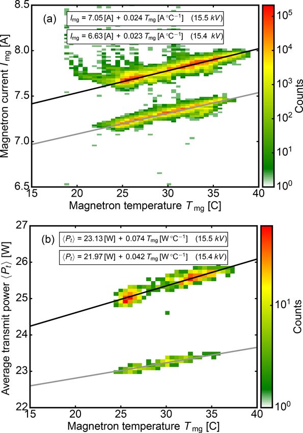
1820                                                                      F. Ewald et al.: Calibration of a 35 GHz airborne cloud radar

                                                                              the received signal S is plotted as a function of the gate num-
                                                                              ber. While connected to the receiver input, the external noise
                                                                              source is switched on and off with signals Son  ∗ (r) (red) and
                                                                                ∗
                                                                              Soff (r) (green) measured in atmospheric gates. Correspond-
                                                                                             ∗ and S ∗ are the signals measured in the two
                                                                              ing to this, Scal      ng
                                                                              last gates, namely the calibration and the receiver noise gates.
                                                                              The in-flight signals in these two reference gates are denoted
                                                                              by Scal and Sng .
                                                                                  Using the so called Y-factor method (Agilent Technolo-
                                                                              gies, 2004), the averaged noise floor ratio Y in atmospheric
                                                                              gates between the external noise source being switched on
                                                                              and off and the ENR of the external noise source is used to
                                                                              determine the noise factor Fn created by the receiver compo-
Figure 2. Total received signal S in digital numbers as a function of
                                                                              nents:
gate number with external noise source switched on (Son    ∗ , red) and               ENR               hS ∗ (r)i
                 ∗ , green). The two last gates monitor the signals
switched off (Soff
                                                                              Fn =          , with Y = on ∗ (r)i                          (13)
                                                                                     Y −1               hSoff
Sng and Scal , which correspond to the receiver noise and the internal
                                                                                                      ∗ (r)i of atmospheric gates is done for
calibration source. The factors c1∗ , c2 and c3∗ correct the estimated        Here, the averaging hSon
noise power Pn† to reflect the actual receiver sensitivity Pn . Signal        gate numbers larger than 10 to exclude the attenuation caused
levels obtained only during the calibration with the external noise           by the transmit–receive switch immediately after the mag-
source are marked with an asterisk.                                           netron pulse. During the initial calibration with the external
                                                                              noise source, a noise figure NF = 8.8 dB was determined.
                                                                                 Summarizing the above considerations, an overall receiver
      More specifically, Pn can be interpreted as an overall re-              sensitivity Pn† is estimated using an assumed receiver noise
      ceiver noise power and is thus equal to the power of the                bandwidth of 5 MHz, a receiver temperature of 290 K and a
      smallest measurable white signal. It includes the inher-                noise figure of NF = 8.8 dB. According to Eq. (12), the es-
      ent thermal noise within the receiver response, the over-               timated receiver sensitivity Pn† used in the initial calibration
      all noise figure of the receiver and mixer circuitry and                is
      all losses occurring between ADC and receiver input.
                                                                              Pn† = −98.2 [dBm].                                           (14)
3.3    Estimated receiver sensitivity
                                                                              The measurements with the external noise source are further-
Prior to this work, no rigorous determination of the receiver                 more exploited to correct for various effects, which cause de-
transfer function T was performed. During the initial calibra-                viations between the inherent noise power Pn† in the noise
tion, the receiver sensitivity Pn was instead estimated using                 gate and the actual receiver sensitivity Pn :
the inherent thermal noise and its own noise characteristic.                  Pn = c1∗ c2 Pn† .                                            (15)
   Generated by thermal electrons, the inherent thermal noise
PkTB received by a matched receiver can be derived using                      Here, the following applies:
Boltzmann’s constant kB , temperature T0 and the noise band-                     – c1∗ accounts for the attenuation in atmospheric gates,
width Bn of the receiver. Additional noise power is intro-                         which is caused by the transmit–receive switch imme-
duced by the electronic circuitry itself, which is considered                      diately after the magnetron pulse:
by the receiver noise factor Fn . The noise factor Fn expressed                                   ∗ (r) − S ∗ (r)i
in decibels (dB) is called noise figure NF. Combined, PkTB                                      hSon       off
                                                                                    c1∗ (r) =     ∗ (r) − S ∗ (r)
                                                                                                                   .                       (16)
and Fn yield the total inherent noise power Pn† :                                                Son       off

Pn† = PkTB Fn = kB T0 Bn Fn [W].                                  (12)              As evident in Fig. 2, c1∗ is only significant in the first
                                                                                    eight range gates (= 240 m) and rapidly converges to
Using a calibrated external noise source with known excess                          0 dB in the remaining atmospheric and reference gates.
noise ratio (ENR), Fn was determined in the laboratory. In-                      – Secondly, the correction factor c2 is used to monitor and
flight, Fn is monitored using the calibration and the noise                        correct in-flight drifts of the receiver sensitivity. To this
gate.                                                                                               ∗ /S ∗ measured during calibration be-
                                                                                   end, the ratio Scal    ng
   In the following, measurements obtained with the cali-                          tween calibration and noise gate is compared to the ratio
brated external noise source in the laboratory are marked                          Scal /Sng during flight:
with an asterisk. Signal levels measured in-flight as well as
                                                                                            ∗ /S ∗
                                                                                           Scal
during the calibration are marked without an asterisk. Fig-                                     ng
                                                                                    c2 =               .                                   (17)
ure 2 shows the external noise source measurements, where                                  Scal /Sng

Atmos. Meas. Tech., 12, 1815–1839, 2019                                                             www.atmos-meas-tech.net/12/1815/2019/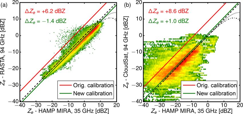
F. Ewald et al.: Calibration of a 35 GHz airborne cloud radar                                                                    1821

      In the course of one flight of several hours, c2 varies          3.4.1   Receiver bandwidth
      only slightly by ±0.5 dB. Continuous observation of c2
      should be performed to keep track of the receiver sensi-         To determine the spectral response, the frequency sweep
      tivity.                                                          mode of the signal generator with a fixed signal amplitude
                                                                       was used within a region of 35 500±20 MHz. For the shorter
  – A further factor accounts for the fact that the noise level        match filter length (τr = 100 ns) on the left and for the longer
    measured in the noise gate is lower than the total system          matched filter length (τr = 200 ns) on the right, Fig. 3 shows
    noise with matched load because the low-noise ampli-               measured signal-to-noise ratios as a function of the frequency
    fier is not matched during the noise gate measurement.             offset from the center frequency at 35.5 GHz. The spec-
    The SNR† determined with the noise gate level there-               tral response of the receiver for both matched filters (black
    fore overestimates the actual SNR in atmospheric gates:            lines) approaches a Gaussian fit (crosses). To estimate the
                                                                       finite receiver bandwidth loss Lfb using Eq. (4), the 6 dB fil-
                                                                       ter bandwidth (two-sided arrow) is determined directly from
      SNR = c3∗ SNR† .                                         (18)
                                                                       the receiver response with B6 = 9.8 MHz for τr = 200 ns and
                                                                       B6 = 17.2 MHz for τr = 100 ns. In the following, the equiv-
      In Fig. 2, this offset is called c3∗ . Its value is determined   alent noise bandwidth (ENBW) concept is used to determine
      by comparing the signal Sng    ∗ in the noise gate with the
                                                                       the receiver noise bandwidth Bn which is needed to calcu-
               ∗
      signal Soff in atmospheric gates, while the external noise       late Pn . In short, the ENBW is the bandwidth of a rectan-
      source is switched off:                                          gular filter with the same received power as the actual re-
               ∗                                                       ceiver. Illustrated by the green and blue hatched rectangles
              Sng                                                      in Fig. 3, the measured ENBW is Bn,200 = 7.5 MHz for the
      c3∗ =    ∗     .                                         (19)
              Soff                                                     longer matched filter length and Bn,100 = 13.5 MHz for the
                                                                       shorter matched filter length. In contrast, the red-hatched
      This offset between noise gate and total system noise            rectangles show the estimated 5 MHz (and 10 MHz) receiver
      remains very stable with c3∗ = −0.83 dB. Since c3∗ exists        noise bandwidth using 1/τr . The discrepancy between the
      only in earlier MIRA-35 systems (without MicroBlaze              measured and the estimated noise bandwidth could be traced
      processor, e.g. KIT, UFS, HALO and Lindenberg), most             back to an additional window function which was applied
      MIRA-35 operators do not have to address this issue.             unintentionally to IQ data within the digital signal processor.
                                                                       This issue led to a bit more thermal noise power PkTB . For
3.4   Measured receiver sensitivity                                    the operationally used matched filter (τr = 200 ns), the offset
                                                                       between estimated and actual thermal noise power (−106.9
A key component of this work was to replace the estimated              vs. −105.2 dBm) led to an 1.8 dB underestimation of Ze . Fu-
receiver sensitivity Pn† with an actual measured value Pn .            ture measurements will not include this bias since this issue
While Pn† was calculated using an assumed receiver noise               was found and fixed.
bandwidth and the receiver noise factor, Pn is now measured
directly using a calibrated signal generator with adjustable           3.4.2   Receiver transfer function
power and frequency output. By varying the power at the re-
ceiver input, Pn is found as the noise-equivalent signal when          Next, the amplitude ramp mode of the signal generator was
SNR = 0 dB. In addition, the receiver response and its band-           used to determine the transfer function Pr = T (SNR) of the
width is determined by varying the frequency of the signal             receiver. The receiver transfer function references absolute
generator. Both measurements are then used to evaluate and             signal powers at the antenna port with corresponding SNR
check Fn according to Eq. (12). This is done for two different         values measured by the receiver. Moreover, the linearity and
matched filter lengths (τr = 100 ns, τr = 200 ns) to character-        cut-offs of the receiver can be assessed on the basis of the
ize the dependence of Bn and Fn on τr .                                transfer function. For this measurement, the frequency of
   To this end, an analog continuous wave signal generator             the signal generator was set to 35.5 GHz, while the output
E8257D from Agilent Technologies was used to determine                 power of the generator was increased steadily from −110 to
the receiver’s spectral response and its power transfer func-          10 dBm. This was done in steps of 1 dBm while averaging
tion T . The signal generator was connected to the antenna             over 10 power spectra. In order to test the linearity and the
port of the radar receiver and tuned to 35.5 GHz, the cen-             saturation behavior of the receiver for strong signals, these
tral frequency of the local oscillator. For the characterization,      measurements were repeated with an internal attenuator set
the radar receiver was set into standard airborne operation            to 15 and 30 dB. For τr = 200 ns, Fig. 4a shows the measured
mode. In this mode, 256 samples are averaged coherently                receiver transfer functions for the three attenuator settings of
into power spectra by FFT. Subsequently, 20 power spectra              0 dB (black), 15 dB (green) and 30 dB (red). For measure-
are then averaged to obtain a smoothed power spectrum for              ments with an activated attenuator, SNR values have been
each second.                                                           corrected by +15 dB (respectively +30 dB) to compare the

www.atmos-meas-tech.net/12/1815/2019/                                                    Atmos. Meas. Tech., 12, 1815–1839, 2019
1822                                                                  F. Ewald et al.: Calibration of a 35 GHz airborne cloud radar

Figure 3. Measured radar receiver response (gray) as a function of the frequency offset from the center frequency at 35.5 GHz for two
different matched filter lengths. While the green and blue hatched rectangles show the actual equivalent noise bandwidths, the red-hatched
rectangles show the estimated noise bandwidth that was used in the initial calibration.

Figure 4. (a) Measured receiver transfer functions for the three attenuator settings of 0 dB (black), 15 dB (green) and 30 dB (red). (b) Linear
regression receiver transfer function to determine the receiver sensitivity Pn .

transfer functions to the one with 0 dB attenuation. The over-            With a slope m of 1.0009 (±0.0006) and a residual of
lap of the different transfer functions between input powers              0.054 dB, the receiver behaved very linearly for this input
of −70 and −30 dBm in Fig. 4a confirms the specified atten-               power region. Similar values were obtained for an attenua-
uator values of 15 and 30 dB. Furthermore, no further satu-               tion of +15 dB with a slope of 0.9980 (±0.0005) and a resid-
ration by additional receiver components (e.g., mixers or fil-            ual of 0.024 dB and a slope of 0.9884 (±0.0013) and a resid-
ters) can be detected up to an input power of −5 dBm. This                ual of 0.1 dB for an attenuation of +30 dB.
allows the dynamic range to be shifted by using the attenua-
tor to measure higher input powers (which would otherwise
be saturated) without losing the absolute calibration. This
feature is essential for the evaluation of very strong signals            3.4.3   Receiver sensitivity
like the ground return.
   Subsequently, a linear regression to the results without an
attenuator was performed between input powers of −70 and
−40 dBm, which is shown in Fig. 4b.                                       Finally, the linear regression to the receiver transfer func-
                                                                          tion can be used to derive the receiver sensitivity Pn . Its x-
SNR = T (Pr ) ≈ mPr − Pn [dB]                                  (20)       intercept (SNR = 0) directly yields the receiver sensitivity Pn

Atmos. Meas. Tech., 12, 1815–1839, 2019                                                       www.atmos-meas-tech.net/12/1815/2019/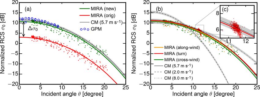
F. Ewald et al.: Calibration of a 35 GHz airborne cloud radar                                                                   1823

for the two matched filter lengths:                                  Table 2. Breakdown of the offset between original and new cali-
                                                                     bration for each system parameter. Values for Lrx+tx and Lfb were
Pn = −92.7 dBm (τr = 100 ns),                                (21)    already known but not applied in past measurement campaigns. The
                                                                     total offset has to be applied to Rc and Ze .
Pn = −95.3 dBm (τr = 200 ns).                                (22)
                                                                             Parameter    Original     This study     Offset
As discussed before, the setting with the shorter matched fil-
                                                                             Lrx+tx       –            1.5 dB         +1.5 dB
ter length collects more thermal noise due to the larger re-
                                                                             Lfb          –            1.2 dB         +1.2 dB
ceiver bandwidth. In a final step, this top-down approach to
                                                                             L2bp         1.0 dB       3.0 dB         +2.0 dB
obtain Pn for different τr can be used to determine Fn and
                                                                             Ga           49.75 dBi    50.0 dBi       −0.5 dB
check for its dependence on τr . By solving Eq. (12) for Fn
                                                                             φa           0.6◦         0.56◦          +0.6 dB
and inserting the measured bandwidths B100 and B200 we ob-                   Pn           −98.2 dBm    −95.3 dBm
tain the following:                                                          NF           8.8 dB       9.9 dB         +1.1 dB
                                                                             Bn           5 MHz        7.5 MHz        +1.8 dB
Pn /PkTB = Fn                                                (23)
                                                                             Total                                    +7.6 dB
− 92.7 dBm + 102.6 dBm = 9.9 dB (τr = 100 ns)                (24)
− 95.3 dBm + 105.2 dBm = 9.9 dB (τr = 200 ns).               (25)
                                                                     4     External calibration using the ocean surface
Remarkably, Fn shows no dependence on τr but turns out to                  backscatter
be larger than previously estimated by 1.1 dB. This previous
underestimation of Fn led to an 1.1 dB underestimation of            The following section will now test the absolute calibration
Ze .                                                                 using an external reference target. As already mentioned in
   Now, all system parameters are known to estimate the              the introduction, the ocean surface has been used as a cali-
radar sensitivity at a particular range. Following Doviak and        bration standard for air- and spaceborne radar instruments. In
Zrnić (2006), the minimum detectable effective reflectivity         their studies, Barrick et al. (1974) and Valenzuela (1978) re-
Zmin (r) at a particular range can be calculated using Eq. (2)       viewed and harmonized theories to describe the interaction of
in decibels:                                                         electro-magnetic waves with the ocean surface. They showed
                                                                     that the normalized radar cross section σ0 of the ocean sur-
                                                                     face at small incidence angles (2 < 15◦ ) can be described
Zmin (r) = MDS + 20log10 r + log10 Rc .                      (26)
                                                                     by quasi-specular scattering theory. At larger incidence an-
                                                                     gles (2 > 15◦ ), Bragg scattering at capillary waves becomes
Here, Pr is the minimum detectable signal (MDS) in dBm               dominant, which complicates and enhances the backscatter-
which is given by Pn SNRmin using Eq. (11):                          ing of microwaves by ocean waves.

MDS = Pn SNRmin .                                            (27)    4.1    Modeling the normalized radar cross section of the
                                                                            ocean surface
In the operational configuration (Q = 7, NP = 256, NS =
20), the MDS is −117.4 dBm, since SNRmin = −22.1 dB and              At the scales of millimeter waves and for small incidence
Pn = −95.3 dBm. The parameters listed in Table 1 yield a             angles θ , the ocean surface slope distribution is assumed to
range-independent radar constant of Rc = 3.9 dB. Using the           be Gaussian and isotropic, where the surface mean square
MDS and Rc in Eq. (26), the minimum detectable effective             slope s(v) is a sole function of the wind speed v and inde-
reflectivity in 5 km is Zmin (5 km) = −39.8 dBZ.                     pendent from wind direction. Backscattered by ocean sur-
                                                                     face facets, which are aligned normal to the incidence waves
3.5   Overall calibration budget                                     (Plant, 2002), the normalized radar cross section σ0 can be
                                                                     described as a function of ocean surface wind speed v and
Comparing the measured Pn = −95.3 dBm to the estimated               beam incidence angle θ (Valenzuela, 1978; Brown, 1990;
Pn† = −98.2 dBm for τr = 200 ns, the combination of band-            Z. Li et al., 2005):
width bias (1.8 dB) and larger noise figure (1.1 dB) caused a                         |0e (0, λ)|2

                                                                                                            tan2 (θ )

2.9 dB underestimation of Ze . Combined with the disregard           σ0 (v, θ, λ) =                  exp  −             .     (28)
                                                                                     s(v)2 cos4 (θ )         s(v)2
of the 2.0 dB higher two-way attenuation by the radome and
the 1.5 dB higher two-way attenuation by the waveguides as           For the ocean surface facets at normal incidence, the reflec-
well as the disregard of the finite receiver bandwidth loss Lfb      tion of microwaves is described by an effective Fresnel re-
                                                                                                         [n(λ)−1]
of 1.2 dB, effective reflectivities derived with the initial cali-   flection coefficient 0e (0, λ) = Ce [n(λ)+1] . In this study, the
bration has to be corrected by +7.6 dB. Table 2 summarizes           complex refractive index n(λ = 8.8 mm) = 5.565 + 2.870i
and breaks down all offsets found in this work.                      for seawater at 25 ◦ C is used following the model by Klein

www.atmos-meas-tech.net/12/1815/2019/                                                    Atmos. Meas. Tech., 12, 1815–1839, 2019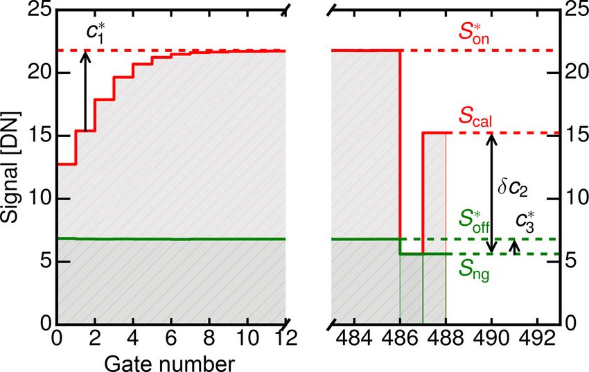
1824                                                              F. Ewald et al.: Calibration of a 35 GHz airborne cloud radar

and Swift (1977). Like with other models (Ray, 1972; Meiss-           included in research flights to implement the well-established
ner and Wentz, 2004), the impact of salinity on σ0 is negligi-        calibration technique to measure the normalized radar cross
ble, while the influence of the ocean surface temperature on          section of the ocean surface at different incidence angles.
σ0 stays below 1σ0 = 0.5 dB between 5 and 30 ◦ C. Since                   During NARVAL2, HAMP MIRA was installed in the
specular reflection is only valid in the absence of surface           belly pod section of HALO and aligned in a fixed nadir-
roughness, various studies (Wu, 1990; Jackson et al., 1992;           pointing configuration with respect to the airframe. The inci-
Freilich and Vanhoff, 2003; L. Li et al., 2005) included a cor-       dence angle is therefore controlled by pitch-and-roll maneu-
rection factor Ce to describe the reflection of microwaves on         vers of the aircraft. The aircraft position and attitude are pro-
wind-roughened water facets. While Ce has been well char-             vided at a 10 Hz rate by the BAsic HALO Measurement And
acterized for the Ku band (Apel, 1994; Freilich and Van-              Sensor System (BAHAMAS; Krautstrunk and Giez, 2012).
hoff, 2003) and W band (Horie et al., 2004; L. Li et al.,             Pitch, roll and yaw angles are provided with an accuracy of
2005), experimental results valid for the Ka band are scarce          0.05◦ , while the absolute uncertainty can be up to 0.1◦ . Addi-
(Nouguier et al., 2016). Tanelli et al. (2006) used simultane-        tional incidence angle uncertainty is caused by uncertainties
ous measurements of σ0 in the Ku and Ka bands, to determine           in the alignment of the radar antenna. Following the approach
|0e (0, λ = 8.8 mm)|2 = 0.455 for the Ka band, which corre-           of Haimov and Rodi (2013), the apparent Doppler velocity of
sponds to an correction factor Ce of 0.90. However, there             the ground was used to determine the antenna beam-pointing
is an ongoing discussion about the influence of radar wave-           vector. With this technique, the offsets from nadir with re-
length or wind speed on Ce (Jackson et al., 1992; Tanelli             spect to the airframe was determined with 0.5◦ to the left in
et al., 2008). Chen et al. (2000) explains this disagreement          the roll direction and 0.05◦ forward in the pitch direction.
with the different surface mean square slope statistics used              During calibration patterns, HALO flew at 9.7 km altitude
in these studies, which do not include ocean surface rough-           with a ground speed of 180 to 200 ms−1 . The pulse repe-
ness at the millimeter scale. To include this uncertainty in          tition frequency was kept at 6 kHz with a pulse length of
this study, the correction factor Ce has been varied between          τp = 200 ns. For the purpose of calibration, the data pro-
0.85 and 0.95, while the simple model (CM) for non-slick              cessing and averaging was set to 1 Hz, being the standard
ocean surfaces by Cox and Munk (1954) was used for s(v).              campaign setting with Doppler spectra averaged from 20
In their model, the surface mean square slope s(v) scales lin-        FFTs, which each contain 256 pulses. As a consequence of
early with wind speed v, describing a smooth ocean surface            this configuration, the ocean surface backscatter at nadir was
including gravity and capillary waves:                                sampled in gates measuring approx. 100 m in the horizontal
                                                                      and 30 m in the vertical. With this gate geometry, a uniform
s(v)2 = 0.003 + 5.08 × 10⁻³ v.                            (29)        beam-filling of the ocean surface is ensured for incidence an-
4.2    Measuring the normalized radar cross section of                gles below 20◦ .
       the ocean surface                                                  In the current configuration, the point target spread func-
                                                                      tion of the matched receiver is under-sampled since the sam-
The ocean surface backscatter is also measured by the Global          pling is matched to the gate length. Thus, the maximum of
Precipitation Measurement (GPM; Hou et al., 2013) platform            the ocean backscatter can become underestimated when the
which carries a Ku- and Ka-band dual-frequency precipita-             surface is located between two gates. At nadir incidence, neg-
tion radar (DPR). For this study, σ0∗ from GPM is used as             ative bias values of σ0 of up to 3–4 dB were observed in ear-
an independent source to support the calculated σ0 from the           lier measurement campaigns, when the gate spacing equals
model. Operating at 35.5 GHz, the KaPR scans the surface              or is larger than the pulse length (Caylor et al., 1997). For this
backscatter with its 0.7◦ beamwidth phased array antenna,             reason, the received power from the range gates below and
resulting in a 120 km swath of 5 km × 5 km footprints. The            above were added to the received power of the strongest sur-
measured ocean surface backscatter by GPM is operationally            face echo. By adding the power from only three gates, Caylor
used to retrieve surface wind conditions and path-integrated          et al. (1997) could reduce the uncertainty in σ0 to 1 dB and
attenuation of the radar beam. In the following, the σ0∗ cor-         exclude the contribution by antenna side-lobes from larger
rected for gaseous attenuation from GPM was used, which               ranges.
corresponds to the co-localized matched swath of the KaPR.                Furthermore, the backscattered signal was corrected for
   During the second Next-Generation Remote Sensing                   gaseous attenuation by oxygen and water vapor considered
for Validation Studies (NARVAL2) in June–August 2016,                 in the loss factor Latm . While the two-way attenuation by
HAMP MIRA was deployed on HALO. The campaign was                      oxygen and water vapor is normally almost negligible in
focused on the remote sensing of organized convection over            the Ka band, it has to be considered in subtropical regions
the tropical North Atlantic Ocean in the vicinity of Barba-           with high humidity and temperature near the surface. To this
dos. Another campaign objective was the integration and val-          end, the gaseous absorption model for millimeter waves by
idation of the new remote sensing instruments on board the            Rosenkranz (1998) was used. Sounding profiles of pressure,
HALO aircraft. For the HAMP MIRA cloud radar, multiple                temperature and humidity were provided by Vaisala RD-94
roll and circle maneuvers at different incidence angles were

Atmos. Meas. Tech., 12, 1815–1839, 2019                                                  www.atmos-meas-tech.net/12/1815/2019/
F. Ewald et al.: Calibration of a 35 GHz airborne cloud radar 1825
Figure 6. Overview of the flight path during the calibration maneu-
ver with the beam incidence angle θ shown by the color map.
Figure 5. Flight track in orange with a true-color image taken dur- ter of each track, with inclination angles θ > 0 left and right
ing that time by the geostationary SEVIRI instrument. The red circle
towards the edges of the swath. Apparently, σ0∗ seems spa-
marks the circular flight section shown in Fig. 6. The superimposed
color map shows the Ka band σ0∗ measured by GPM in the vicinity
tially quite homogeneous, where the ocean surface is only
of the operating area. covered by small marine cumulus clouds. The first way-
point was chosen to be collocated with a meteorological buoy
(14.559◦ N, 53.073◦ W, NDBC 41040) to obtain the accurate
dropsondes, which were launched from HALO during the wind-speed and direction at the level of the ocean surface as
calibration maneuvers. well as wave heights measured by the buoy. At 12:50 UTC,
Following L. Li et al. (2005), the measured normalized the buoy measured a wind speed of 5.7 m s−1 from 98◦ with
cross section σ0∗ of the ocean surface can be calculated from a mean wave height of 1 m and mean wave direction of 69◦ .
measured signal-to-noise ratios: A detailed overview of the flight path during the calibration
maneuver is shown in Fig. 6, where the beam incidence an-
cπ 5 τp Rc r 2 L2atm gle θ is shown by the color map. At 12:40 UTC, the air-
σ0∗ = Pn SNR. (30)
2λ4 1018 craft executed a set of ±20◦ roll maneuvers to sample σ0∗
Here, the receiver power Pr was replaced with Pn SNR in the cross-wind direction. At 12:44 UTC, the aircraft en-
(Eq. 10) to include the overall receiver sensitivity Pn in the tered a right-hand turn with a constant roll angle of 10◦ , the
formulation of σ0∗ . Like in Eq. (2), Rc is the radar constant incidence angle for which σ0∗ becomes insensitive to surface
(with |K|2 = 1) which includes the transmitter power Pt , wind conditions and models. After a full turn at 12:58 UTC,
transmitting and receiving waveguide loss Ltx and Lrx , at- another set of ±20◦ roll maneuvers were executed to sample
tenuation by the belly pod Lbp and the antenna gain Ga . To- σ0∗ in the along-wind direction. The dropsonde was launched
gether with Pn , the combination of these system parameters around 13:06 UTC at 12.98◦ N and 52.78◦ W. A two-way
are being checked in the following section, when the mea- attenuation by water vapor and oxygen absorption L2atm of
sured σ0∗ is compared to the modeled σ0 . For the following 0.78 dB was calculated using the dropsonde sounding. With
analysis, σ0∗ was obtained with Eq. (30) using 1 Hz averaged an approximate distance of 700 km, the GPM measurement
SNR from HAMP MIRA. closest to the calibration area was made at 10:46:29 UTC at
13.67◦ N and 59.53◦ W. To obtain a representative σ0∗ mea-
4.3 Comparison of measurements and model surement from GPM, the swath data were averaged along-
track for 10 s.
The HAMP MIRA calibration maneuver during NARVAL2 The measurement of σ0∗ during the across-wind roll ma-
was included in research flight RF03 on 12 August 2016. The neuver is shown in Fig. 7a. The blue circles mark the corre-
flight took place 700 km east of Barbados in a region of a rel- sponding GPM measurements. For the HAMP MIRA data,
atively pronounced dry intrusion with light winds and very σ0∗ was calculated using the old, estimated calibration (red
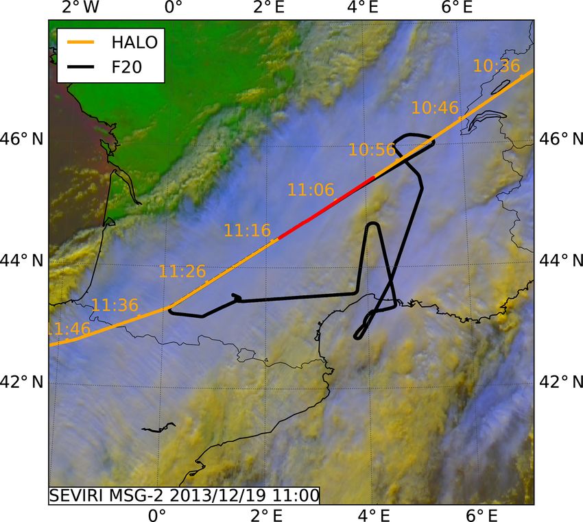
little cloudiness. Figure 5 shows the flight track in orange dots) and the new, measured calibration (green dots). In or-
with a true-color image taken during that time by the geo- der to assess the agreement of σ0∗ with σ0 , the CM model
stationary SEVIRI instrument. The superimposed color map for σ0 (Eq. 28) was first calculated using the measured wind
shows σ0∗ from GPM in the vicinity of the operating area speed from the buoy. These values are shown by the black
for that day. Here, the satellite nadir is located in the cen- line in Fig. 7a. The shaded region around this line illustrates
www.atmos-meas-tech.net/12/1815/2019/ Atmos. Meas. Tech., 12, 1815–1839, 20191826 F. Ewald et al.: Calibration of a 35 GHz airborne cloud radar
Figure 7. Normalized radar cross section (RCS) σ0∗ of the ocean surface as a function of the radar beam incident angle θ . (a) Falloff of
σ0∗ with θ measured with HAMP MIRA (red/green dots) and GPM (blue circles). The HAMP MIRA data are calculated and subsequently
fitted using the old, estimated calibration (red line) and the new, measured calibration (green line). The modeled value (CM: Cox–Munk)
and uncertainty of σ0 for the actual measured wind speed from the buoy is shown by the black line and the shaded region. (b) Comparison
of measured σ0∗ during the along-wind (orange) and across-wind (green) roll maneuver and during the turn (red). (c) A closer look on the
scatter of σ0 during the turn maneuver, with a standard deviation of 0.8 dB.
the uncertainty in σ0 due to the uncertainty in Ce (0.85 . . . footprint, with more ocean surface facets pointing into the
0.95). Both modeled and measured σ0 show the exponential backscatter direction. The much better agreement of the new
falloff with θ corresponding to the smaller mean square slope absolute calibration with GPM is a further demonstration of
of the ocean surface with increasing θ . In a second step, the its validity.
CM model was fitted to σ0∗ from the old (red line) and new Extending this discussion, the dependence of σ0∗ on wind
(green line) calibration to obtain the wind speed v. Here, a direction is tested in the following study. To this end, Fig. 7b
potential calibration offset 1σ0 was considered as a second shows σ0∗ measured during the across-wind (green) and
fitting parameter: along-wind (red) roll maneuver as well as during the turn.
Like in Fig. 7a, the CM model for the actual measured wind
σ0∗ = σ0 (v, θ, λ) + 1σ0 , (31) speed of 5.7 m s−1 is fitted to the 1 Hz averaged σ0∗ measured
during the three flight patterns. While the across-wind results
The following analysis is valid for the turn maneuver; dif- are slightly below the values of σ0 predicted by the wind
ferences between across-wind roll, turn and along-wind roll speed of the buoy by 1σ0 = −0.5 dB, the along-wind results
maneuver are discussed in the Fig. 7b and the following para- underestimate σ0 by 1σ0 = −0.8 dB. In comparison, the fit
graph. For old and new calibration, the fitted wind speed of to the measurements in the turn showed the smallest offset
5.71 m s−1 agrees very well with the actual measured wind 1σ0 = −0.2 dB. The inset in Fig. 7c gives a closer look on
speed of 5.7 m s−1 . While σ0∗ for the old calibration shows a the scatter of σ0 during the turn maneuver, with a standard
strong underestimation of σ0 by 1σ0 = −7.8 dB, the fit for deviation of 0.8 dB. Here, the slightly higher values were
the new calibration only marginally underestimates σ0 with measured in the downwind section of the turn; an observation
1σ0 = −0.2 dB, well within the uncertainty of σ0 . Thus, that is in line with measurements by Tanelli et al. (2006). In
the initial calibration yields 7.6 dB smaller values for σ0∗ addition, this scatter is further caused by the under-sampled
when compared to the new calibration that is in good agree- point target spread function of the ocean surface with a re-
ment with the modeled values. This observed difference also maining uncertainty of 1 dB. Due to these two effects, the
matches precisely with the 7.6 dB difference determined dur- measured σ0∗ will be associated with an uncertainty of 1 dB.
ing the absolute calibration in Sect. 3. Furthermore, the ac- To put a possible directional dependence in perspective to
curacy of the new absolute calibration is supported by the the effect of different wind speeds, modeled σ0 are plotted
GPM measurements in the vicinity. With an increasing offset with their uncertainty for wind speeds of 2 m s−1 (dashed
1σ0 from −0.1 dB to −1 dB towards smaller incidence an- line), 8 m s−1 (dashed–dotted line) and the actual 5.7 m s−1
gles, GPM measured only slightly larger values within its 9◦ (solid line). In summary, measured σ0∗ for the new calibra-
co-localized matched swath compared to the new absolute tion agree with modeled as well as independently measured
calibration. Here, the small, increasing offset 1σ0 with de- values within their uncertainty estimates.
creasing θ suggests a slightly lower wind speed at the GPM
Atmos. Meas. Tech., 12, 1815–1839, 2019 www.atmos-meas-tech.net/12/1815/2019/You can also read