Radar-based assessment of hail frequency in Europe - Natural Hazards and Earth System Sciences
←
→
Page content transcription
If your browser does not render page correctly, please read the page content below
Nat. Hazards Earth Syst. Sci., 21, 683–701, 2021
https://doi.org/10.5194/nhess-21-683-2021
© Author(s) 2021. This work is distributed under
the Creative Commons Attribution 4.0 License.

Radar-based assessment of hail frequency in Europe
Elody Fluck1,a , Michael Kunz1,2 , Peter Geissbuehler3 , and Stefan P. Ritz3
1 Instituteof Meteorology and Climate Research (IMK), Karlsruhe Institute of Technology (KIT), Karlsruhe, Germany
2 Center for Disaster Management and Risk Reduction Technology (CEDIM), Karlsruhe, Germany
3 RenaissanceRe Risk Sciences, Zurich, Switzerland
a now at: Department of Earth and Planetary Sciences, Weizmann Institute of Science, Rehovot, Israel

Correspondence: Elody Fluck (elody.fluck@weizmann.ac.il)

Received: 23 April 2020 – Discussion started: 3 June 2020
Revised: 11 January 2021 – Accepted: 14 January 2021 – Published: 17 February 2021

Abstract. In this study we present a unique 10 year climatol-    land (e.g., Dessens, 1986; Puskeiler et al., 2016; Nisi et al.,
ogy of severe convective storm tracks for a large European       2016). Prominent examples are the two hailstorms related
area covering Germany, France, Belgium and Luxembourg.           to the low-pressure system Andreas that occurred on 27–
For the period 2005–2014, a high-resolution hail potential       28 July 2013 over central and southern Germany with total
composite of 1 × 1 km2 is produced from two-dimensional          economic losses estimated at approximately EUR 3.6 billion
radar reflectivity and lightning data. Individual hailstorm      (SwissRe, 2014; Kunz et al., 2018). Hail occurs in organized
tracks as well as their physical properties, such as radar re-   convective storms (Auer, 1972), that is, multicells, supercells
flectivity along the tracks, were reconstructed for the entire   or mesoscale convective storms (Markowski and Richardson,
time period using the Convective Cell Tracking Algorithm         2010). Hail can also be produced by single-cell pulse storms;
(CCTA2D).                                                        however, large hail is almost always associated with orga-
   A sea-to-continent gradient in the number of hail days per    nized convection, particularly supercells (Smith et al., 2012;
year is found to be present over the whole domain. In ad-        Wapler et al., 2016), and results from the interaction between
dition, the highest number of severe storms is found on the      diverse processes and mechanisms on different spatiotempo-
leeward side of low mountain ranges such as the Massif Cen-      ral scales. Several authors have studied environmental condi-
tral in France and the Swabian Jura in southwest Germany. A      tions favoring hail production (Dessens, 1986; Houze, 2014;
latitude shift in the hail peak month is observed between the    Kunz et al., 2020, among others). In general, a subtle inter-
northern part of Germany, where hail occurs most frequently      play between three main ingredients supports the formation
in August, and southern France, where the maximum amount         of deep moist convection (Kunz, 2007): (1) conditional in-
of hail is 2 months earlier. The longest footprints with high    stability is needed for lifted parcels of air to become pos-
reflectivity values occurred on 9 June 2014 and on 28 July       itively buoyant (2) a high moisture content in lower atmo-
2013 with lengths reaching up to 500 km. Both events were        spheric levels lowers the level of free convection (LFC) in
associated with hailstones measuring up to 10 cm diameter,       a cloud and increases convective available potential energy
which caused damage in excess of EUR 2 billion.                  (CAPE) and (3) a lifting mechanism to trigger convection
                                                                 such as orographic lifting (Kirshbaum et al., 2018; Barthlott
                                                                 et al., 2016) or lifting associate with synoptic cold fronts
                                                                 (Kunz et al., 2020). Vertical wind shear is another parameter
1   Introduction                                                 mainly relevant for the organization form of the storm and,
                                                                 thus, also for its lifetime and severity. Several authors have
Severe convective storms (SCSs) and their related hail con-      found that large hail preferably occurs in strongly sheared en-
stitute a major atmospheric hazard. These events have the        vironments, supporting the formation of supercells (Brooks
potential to cause substantial damage to hail-susceptible ob-    et al., 2003; Johnson and Sugden, 2014; Taszarek et al., 2017;
jects such as buildings, crops or automobiles in various parts   Kunz et al., 2020; Pilorz and Łupikasza, 2020). Aside from
of Europe, including France, Germany, Austria and Switzer-

Published by Copernicus Publications on behalf of the European Geosciences Union.
684                                                      E. Fluck et al.: Radar-based assessment of hail frequency in Europe

the parameters mentioned above, some authors have found            the coastal slopes of the Great Dividing Range. In Czechia,
that an increased frequency of SCSs in Europe can be associ-       Skripniková and Řezáčová (2014) used the Waldvogel crite-
ated with specific large-scale flows or teleconnection patterns    rion on single-polarization radar data to retrieve hail signals
(Piper et al., 2019; Mohr et al., 2019; Kunz et al., 2020). Sev-   for the period 2002 until 2011. The authors found that hail
eral authors found, for example, a configuration where the         occurred mostly during May, June and July during the af-
east of the Atlantic basin is dominated by a low pressure area     ternoon throughout the country. Despite the use of improved
and where France lies under a ridge (Piper et al., 2019; Fluck,    radar-based techniques, most of the studies cited above were
2018).                                                             restricted to smaller regions or a single country. While some
   A major obstacle when investigating hail events and their       authors have estimated hail frequency from other sources
climatology is the lack of accurate and comprehensive ob-          such as overshooting tops (an indicator of strong convective
servations. This observation deficit is because of the local-      updrafts) in satellite imagery (Punge et al., 2014), model data
scale nature of SCSs and the even smaller hailstreaks with a       (Mohr et al., 2015a, b; Rädler et al., 2018) or a combination
small spatial extent (Changnon, 1977). There are only some         thereof (Punge et al., 2017), radar proxies have a key ben-
high-density, regional-scale, ground-detection networks us-        efit over overshooting tops as they represent a more direct
ing hailpads for recording hail fall in operation, such as         measure of hail within a storm (presence of large reflectiv-
in southwestern and central France (Dessens, 1986; Vinet,          ities). Numerical models, such as weather forecast models
2001), parts of Spain (Fraile et al., 1992) and northern Italy     or regional climate models (RCMs), on the other hand, are
(Eccel et al., 2012). The majority of Europe, however, re-         not able to reliably reproduce hail due to a high degree of
mains uncovered by a hail network, leading to a gap in direct      uncertainty in the initial conditions, a lack of knowledge in
hail observations. Therefore, little is known about the local-     cloud microphysics and the high computer costs when run-
scale hail probability and related hail risk across Europe.        ning a two- or three-moments microphysics scheme. The
   Numerous authors have used hail signals derived from            big advantage of satellite or model-based hail proxies is that
conventional weather radars for the identification and anal-       they cover large areas more or less homogeneously, whereas
ysis of hail because of their high temporal and spatial res-       radar-based climatologies are typically limited to a single
olutions. For example, Nisi et al. (2016, 2018) established a      country or region.
hail climatology for Switzerland from 2002 to 2014 based on           Our study is the first to combine radar observations from
both the probability of hail (POH) and maximum expected            multiple countries. Indeed, the objective of our study is to
severe hail size (MESHS) estimated from volumetric (3D)            analyze the spatiotemporal variability of hail signals over a
radar data. Puskeiler et al. (2016) used 3D radar reflectiv-       10 year period (2005 to 2014) covering the four European
ity together with modeled melting layer, lightning data and        countries of France, Germany, Belgium and Luxembourg.
the cell-tracking algorithm TRACE3D (Handwerker, 2002)             Hail signals were estimated from 2D radar reflectivity avail-
to reconstruct hailstreaks and, from that, to estimate the hail    able for each country, which permits a homogeneous hail
frequency across Germany between 2005 and 2011. By com-            analysis. The results help us identify regions frequently af-
bining 3D radar reflectivity and insurance loss data for build-    fected by hail and allow us to relate hail frequency to topo-
ings, Kunz and Puskeiler (2010) it was found that the highest      graphic features such as terrain height or the proximity to the
hail frequency in southwest Germany is located downstream          sea. A thorough study of hail events gives further insights
of the Black Forest mountains. This hotspot was also con-          into the relation between orography and deep moist convec-
firmed by Kunz and Kugel (2015) using five different hail          tion. Improved understanding of these mechanisms and pro-
criteria based on 2D and 3D radar reflectivities and different     cesses is crucial for improving the nowcasting and forecast-
heights (melting layer, echo top). Lukach et al. (2017) com-       ing skill of hailstorms. Finally, as hail constitutes a consid-
puted a hail frequency map for Belgium from 2003 to 2012           erable risk for the insurance industry, improved knowledge
using 3D radar data. Outside of Europe, Cintineo et al. (2012)     about hail frequency and hailstorm characteristics will help
produced a high-resolution hail frequency map for the USA          us better understand the related risks.
from 2007 to 2010 using MESH (Maximum Expected Size                   The paper is structured as follows: Sect. 2 gives an
of Hail) product. The authors found a high hail frequency          overview of the remote-sensing and reanalysis datasets used
during March to September (with June as a maximum) in              for this study. Section 3 describes the combination of radar
the Great Plains. More precisely, the highest hail frequency       data with lightning data and the application of the tracking
is mainly centered over the southern part of the Great Plains      algorithm. The remote-sensing output is then used to gener-
from March until May, while from July to September hail is         ate European composites at 5 min time steps. Section 4 as-
more frequent in the central and northern plains. The MESH         sesses the hail variability between 2005 to 2014 in relation
product was also used in the studies conducted by Warren           to the distance to the sea and the presence of orography near
et al. (2020) in Australia where the authors used daily grids      hailstorms. This section also presents results on seasonal and
of merged radar data including MESH at a 1 km resolution           diurnal variations in hail frequency and provides some char-
from 2009 until 2017. A pronounced peak of hail appeared           acteristics of the hail cells. Concluding remarks follow in
during (Southern Hemisphere) summertime in December on             Sect. 5.

Nat. Hazards Earth Syst. Sci., 21, 683–701, 2021                                   https://doi.org/10.5194/nhess-21-683-2021
E. Fluck et al.: Radar-based assessment of hail frequency in Europe 685
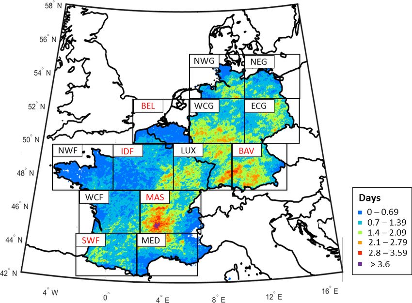
Figure 1. European regions and mountain ranges mentioned in this study.
2 Datasets 2.1.1 French radar data
2.1 Remote-sensing data The French radar network operated by Météo-France and
the derived radar products evolved constantly through time,
In this paper, we present a hail climatology retrieved from
mainly via national projects. A brief overview of the French
radar reflectivity datasets available from the first phase of
radar network is given here. In 2001, 19 radars constituted
the project HAMLET (Hail Model for Europe by Tokio Mil-
the French radar network. One year later, in 2002, five new
lennium) that lasted from 2013 until mid-2017. 2D radar
radars were added to the network and some of the 19 radars
reflectivity for the summer half years (April to September)
were replaced by dual polarization radars (Tabary et al.,
from 2005 to 2014 for Germany, France, Belgium and Lux-
2006; Bousquet et al., 2008). In 2005, 24 radars were in op-
embourg are considered (Fig. 1). The French national radar
eration including 19 C-band radars and five S-band radars
composites were available until 2014 only, due to the instal-
(both with a radius of up to 120 km). Two years later, in 2007,
lation of five new X-band radars in the alpine region in 2014
the radar stations of Toulouse in southwestern France and
(see Sect. 2.1.1), which required some additional time to cal-
Trappes (near Paris) were renewed (Tabary, 2007), but this
ibrate each X-band radar and to implement their data into the
replacement did not affect the radar national composite. Dur-
national radar composite. The French national radar com-
ing the period from 2007 to 2011, the radars of Plabennec lo-
posites from 2015 onward, including the X-band radars in
cated in northwestern France, Abbeville in northern France,
the alpine region installed in 2014, were only available later.
Nimes in southern France and Grèzes in the southern part of
The radar products used in this study are composites of the
central France were replaced with dual polarization radars as
Maximum Constant Altitude Plan Position Indicator (Max-
well. In 2014, five X-band radars with an average coverage
CAPPI), where the composite is a merger of the data from all
radius of 50 km were added to the French national radar com-
local radar stations in a single image at time steps of 5 min.
posite in the alpine region (Beck and Bousquet, 2013; Cham-
2D radar data are used here because of the large domain and
peaux et al., 2011). As the data from the X-band radars were
their long-term availability.
only recently implemented into the French national compos-
ite (Yu et al., 2018), only S- and C-band radars were con-
sidered in this study. Note that the radar stations of Avesnois
(located in northern France) and Réhicourt-la-petite in Lor-
https://doi.org/10.5194/nhess-21-683-2021 Nat. Hazards Earth Syst. Sci., 21, 683–701, 2021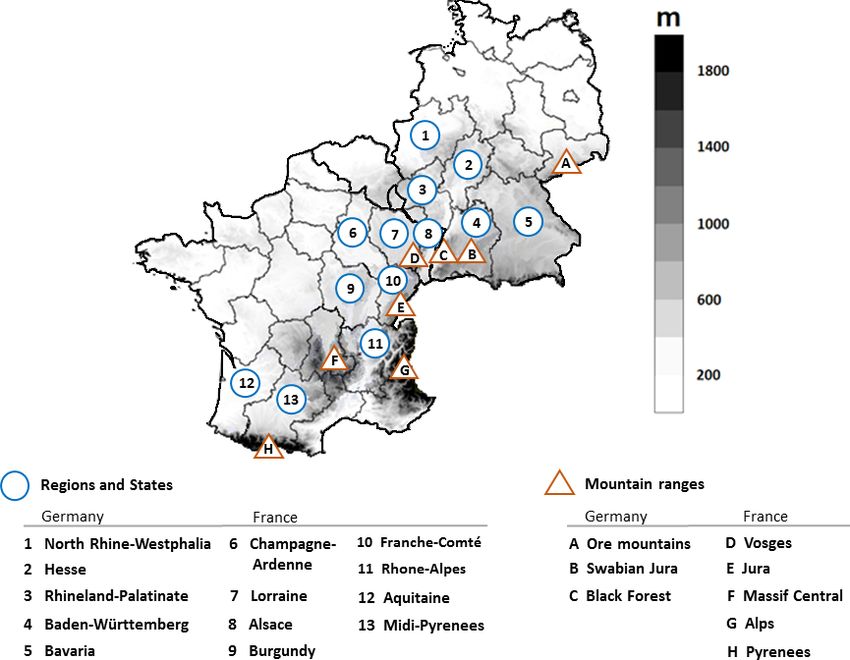
686                                                             E. Fluck et al.: Radar-based assessment of hail frequency in Europe

                                                                           to the radar (Doviak and Zrnić, 2006). For example, a cor-
                                                                           rection of 1.79 dBZ at 100 km away from the radar site is ap-
                                                                           plied to C-band radars for an elevation angle of 0.4◦ (Tabary
                                                                           et al., 2013). One of the last preprocessing steps is the cor-
                                                                           rection of the bright band with the help of vertical reflectiv-
                                                                           ity profiles. After performing all the steps described above,
                                                                           individual plan position indicators (PPIs) are combined to
                                                                           2D composites produced every 5 min available for each radar
                                                                           station. All individual radar products are then combined into
                                                                           a national mosaic (Augros et al., 2013). For areas with over-
                                                                           lapping radar coverage, weighted reflectivity data are com-
                                                                           puted depending on the distance to the nearest radar (Tabary
                                                                           et al., 2013). At the borders of France, radar data from other
                                                                           national weather services are integrated into the French na-
                                                                           tional mosaic. Reflectivity values from the French radar mo-
                                                                           saic used in this study were coded in a table and stored in
                                                                           GeoTIFF format, i.e., georeferenced TIFF images. The res-
                                                                           olution is 2 × 2 km2 from 2004 until mid-June 2009, and a
                                                                           finer resolution of 1×1 km2 is available from mid-June 2009
Figure 2. Locations (squares) and coverage of the radar stations
                                                                           to 2014. For data homogenization, each of the 2×2 km2 com-
(circles) in 2014 used in this study. See text for further explanations.   posites was interpolated linearly from 2004 to June 2009 to
                                                                           the finer grid of 1 × 1 km2 .

                                                                           2.1.2   German radar data
raine (labeled as 7 in Fig. 1) cover a large part of eastern
France and permit the complete integration of Luxembourg,                  The German radar composites for the period from 2005 to
as well as a significant part of Belgium, into the French na-              2014 are provided by the German Weather Service (DWD),
tional composite.                                                          which operated a network of 17 C-band radar systems in
   Concerning the scanning strategy, four to six scans are per-            2014. During the investigation period, a new radar in Mem-
formed every 15 min at elevation angles ranging from 0.4 up                mingen, southern Germany, was added to the network in
to 15◦ (Figueras i Ventura and Tabary, 2013). Only lower el-               2012 (Puskeiler, 2013). As the horizontal range detection for
evation angles below 2.7◦ are scanned every 5 min. The spa-                each radar is 180 km and a maximum distance of 200 km sep-
tial resolution of the composite is 1 × 1 km2 with a size of               arates the radar stations, an extensive overlap of the detection
1536 × 1536 grid points for each image referenced to a plane               areas permits almost a complete coverage of the German ter-
Cartesian coordinate system (Tabary et al., 2006). Radar data              ritory. Only some peripheral regions are not well covered by
from all stations are preprocessed via an algorithm (Tabary,               the composite, for example, in the far north near the Danish
2007) named Castor2 (Figueras i Ventura et al., 2012), which               border and in southeastern Bavaria (Fig. 2). In the complex
corrects for several errors, such as antenna positioning er-               terrain of southern Germany, weather radars are preferably
rors, and quantifies horizontal reflectivity Zh in polar coor-             located on hills and mountains to minimize beam shielding
dinates (Tabary, 2007). During the preprocessing stage, each               by orography. Concerning the scanning strategy, the lowest
radar pixel receives a weighted quality index (QI) ranging                 elevation angles between 0.5 and 1.8◦ (Bartels et al., 2004)
from 0 to 1 (Tabary, 2007), updated throughout the whole                   at that time were scanned every 5 min, whereas a complete
preprocessing chain. The first preprocessing step is to elim-              volume scan took 15 min. The maximum reflectivity values
inate ground clutter, i.e., fixed echoes at the surface, using             of the lowest elevations are used for the national 2D reflec-
Doppler velocity (Tabary et al., 2013). Then an orographic                 tivity composite. The preprocessing steps are similar to those
mask is applied at each elevation angle in order to assess the             of Météo-France and include, among others, an elimination
beam occultation rate. After that, an “anthropogenic” mask,                of clutter pixels using a clutter filter and orographic shad-
including buildings, trees or other fixed objects in the vicin-            ing correction using an elevation model. After preprocess-
ity of the radar is computed with the help of long-term ac-                ing, the local radar data are merged into the German national
cumulated radar products. These masks allow one to remove                  composite. For areas with overlapping radar coverage, the
radar pixels with artificially high reflectivity at each eleva-            maximum reflectivity value from all radar scans is used in
tion angle. The underestimation of reflectivity above the 0 ◦ C            the composites, while for the neighboring regions of foreign
isotherm is taken into account (Tabary et al., 2013) using ver-            countries, a weighted adjustment is performed between radar
tical reflectivity profiles. Attenuation by oxygen is corrected            products from other national weather services and the Ger-
depending on the wavelength, the elevation and the distance                man rain-gauge dataset (Kreklow et al., 2020). The quality

Nat. Hazards Earth Syst. Sci., 21, 683–701, 2021                                            https://doi.org/10.5194/nhess-21-683-2021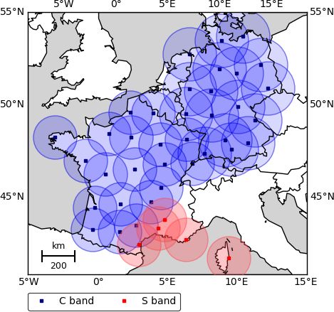
E. Fluck et al.: Radar-based assessment of hail frequency in Europe                                                            687

of German radar data has improved over the last decade with        2.1.4    Lightning data
continuous algorithm corrections and adjustments (Kreklow
et al., 2020) used for RADOLAN (Radar-Online-Aneichung,            To remove artificial clutter still present in the data, we addi-
which means Radar Online Adjustment) and can be assessed           tionally implemented a filter based on lightning data, which
by a quality flag provided for each pixel on the reflectivity      was already used by Puskeiler et al. (2016). Here we used
product. The spatiotemporal resolution as well as the time         only cloud-to-ground (CG) lightning (strokes) from the low-
period available for the German radar data are the same as         frequency lightning detection system BLIDS (BLitz Infor-
for the French data, namely 1 × 1 km2 with a 5 min time step       mationsDienst Siemens), which is part of the EUCLID (EU-
for the composite and available from 2005 until 2014, so both      ropean Cooperation for LIghtning Detection) network. The
data sets can be merged. The encryption of each scan of the        detection efficiency of the system is 96 % for strokes with a
DWD network entails near-ground reflectivity values (named         peak current of at least 2 kA (Schulz et al., 2016). Because
RX products) in so-called RVP6 units. The advantages of            the sensors and the algorithm implemented until 2015 had
these data are the high temporal and spatial resolution, which     a significantly lower detection efficiency of intracloud and
enables us to properly identify footprints of SCSs. RX data        cloud-to-cloud lightning according to Pohjola and Mäkelä
are projected on a Cartesian grid so that each grid box is         (2013), these types of lightning were not considered.
equidistant at 1.0 km. In the end, the German radar composite
has a size of 900 × 900 km2 covering the whole of Germany.         2.1.5    ERA5 reanalysis

2.1.3   Uniform pan-European grid                                  To assess the mean wind flow during hail days, we used the
                                                                   ERA5 global reanalysis (Hersbach et al., 2020). ERA5 is a
It is important to note some limitations in both the German        new global atmospheric reanalysis recently released by the
and French national composites. Long-term QPE (Quantita-           ECMWF and aims to replace ERA-Interim reanalysis (Dee
tive Precipitation Estimation) maps for the French national        et al., 2011) whose data extend from 1979 to 2019. For the
composite reveal some regions with low data accuracy. This         moment, ERA5 is available from 1979 onwards and will be
is mainly the case for the central and eastern part of the Pyre-   soon extended to 1950. The ERA5 4D-Var analysis dataset is
nees mountains and the entire alpine region (Tabary et al.,        assimilated by the Integrated Forecasting System (IFS) and is
2013). In the other parts of France, the QI is mostly higher       available on a horizontal resolution of 0.25◦ on 137 vertical
than 90 % with especially high QIs close to the radar site         levels every hour.
(Tabary et al., 2013). Radar data failure, for example dur-
ing radar calibration or radar replacement, was estimated by
                                                                   3     Methods
Puskeiler et al. (2016) to be approximately 4.5 % ± 3.9 % on
average (mean ± standard deviation for the German national         3.1     Correction of erroneous signals
composite). Furthermore, the combination of the German
and French national composites, each calibrated and prepro-        Concerning the homogenization of the French and German
cessed in different ways, may lead to inhomogeneities in rel-      national composites, several corrections had already been
ative hail frequency in some regions. Based on manual inves-       performed by both national meteorological services. Radar
tigation of several cases with severe hailstorms in the bor-       reflectivity data still contain noise and systematic errors
der region between Germany and France, it was found that           that have to be eliminated using various approaches. Er-
the signal of the French mosaic is between 0.5 and 1 dBZ           rors mostly concern individual radar pixels with significantly
lower compared to that obtained from the DWD composite             higher reflectivity values (e.g., more than 70 dBZ) compared
(Schmidberger, personal communication, 2020). This uncer-          to the surroundings. To avoid this problem, reflectivities be-
tainty is acceptable when projecting the two national com-         low 35 dBZ or above 70 dBZ were set as missing values.
posites onto a uniform pan-European grid. Radar reflectivity       Following Puskeiler et al. (2016), an additional verification
data and thus radar-derived hail signals were projected on the     and correction filter was applied for reflectivity values of
same uniform European grid (not shown) with a resolution           Z > 45 dBZ with a difference of 1Z > 5 dBZ to the adja-
identical to that of the national radar network (1×1 km2 ). We     cent pixels. The affected pixel is set to the mean value of
used the geographic coordinate system WGS84 for the pan-           its eight surrounding pixels and this filter was applied to all
European grid and a Lambert conformal conic projection,            consecutive radar scans:
as recommended by Gregg and Tannehill (1937) and Varga
(1990). In the center, at about 47◦ N and 6◦ E, the meridional                                                           !
grid spacing is equal to the zonal direction to minimize the                       1 X
                                                                                     1
                                                                             1     X
grid distortion.                                                   Z(x, y) =                    Z(x + i, y + j ) − Z(x, y) .   (1)
                                                                             8     i=−1 j =−1

                                                                   In addition, if a reflectivity value at a given grid point is at
                                                                   least twice as high compared to the eight neighboring val-

https://doi.org/10.5194/nhess-21-683-2021                                     Nat. Hazards Earth Syst. Sci., 21, 683–701, 2021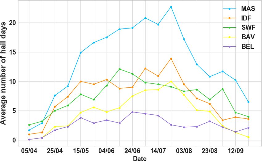
688                                                        E. Fluck et al.: Radar-based assessment of hail frequency in Europe

Table 1. Thresholds required in radar composites to identify poten-   within each ROIP, a value of 1Z = 10 dBZ is subtracted
tial convective cells with the CCTA2D algorithm.                      from Zmax to set the minimum threshold necessary to de-
                                                                      limit an single RC (Zrc ). Thus, the value of Zrc remains the
  Description                                     Value    Units      same for all identified RCs inside a ROIP. If Zrc is less than
  Minimum reflectivity of an ROIP                    35    dBZ        55 dBZ, the RC is rejected and not tracked by CCTA2D. Two
  Minimum reflectivity of an RC                      55    dBZ        additional conditions are required for an RC to be classified
  Reflectivity to subtract from ROIP maximum         10    dB         as a potential convective cell and to be tracked by CCTA2D:
  Minimum RC area                                     5    km2        a minimal area of 5 km2 is needed to define an RC with at
  Minimum number of pixels inside an RC               3    km2        least 3 px (pixels) (km2 ) of Z ≥ 55 dBZ. The thresholds de-
                                                                      tailed above to identify potential convective cells in CCTA2D
                                                                      are summarized in Table 1. The 55 dBZ threshold is referred
                                                                      to as the hail criterion according to Mason (1971) and was
ues and was not present in the scan before or afterward, the
                                                                      successfully used in several studies (e.g., Hohl, 2001; Hohl
reflectivity value is considered an artifact and set to zero.
                                                                      et al., 2002; Kunz and Kugel, 2015). Schuster et al. (2005),
3.2   Lightning filter                                                for example, found 55 dBZ to be a good indicator for dam-
                                                                      aging hail on the ground in eastern Australia. Puskeiler et al.
Although the radar tracking routine (see next paragraph)              (2016) estimated a slightly higher threshold of 56 dBZ to best
includes a clutter filter, several erroneous signals are still        differentiate between days with and without insured dam-
present in the radar data. For example, isolated nonmeteo-            age to buildings but confirmed that 55 dBZ best estimates
rological targets such as electronic signals or reflectivities        insured damage to crops. Categorical verification using in-
from wind turbines can emerge in radar scans (Steiner and             surance loss data over a 7 year period in southwest Germany
Smith, 2002). Since hail occurs only in association with thun-        for this threshold yields a Heidke skill score (HSS) of 0.6,
derstorms (Baughman and Fuquay, 1970; Changnon, 1999;                 a quite high value confirming the detection skill (it should
Wapler, 2017), lightning is expected near high reflectivity           be noted that this value increases to HSS = 0.71 when using
cores. In addition to the gradient filter described above, we         an adjusted version of the Waldvogel et al. (1979) criterion
used lightning detections to further remove artificial clut-          requiring 3D radar data). In the same study, Puskeiler et al.
ter. If high reflectivity values (Z ≥ 55 dBZ) occur during a          (2016) found that the probability of detection (POD) reached
24 h period without lightning, the values at the affected grid        0.65 and the false alarm ratio (FAR) was 0.4, indicating that
points are set to zero. A maximum distance of 10 km was               35 % of the observed hail events are missing while 40 % of
chosen between a lightning discharge location and the pixels          those predicted events are false alarms.
with high reflectivity. Distances of 5, 15 and 20 km were also           The second step of CCTA2D is the temporal and spatial
tested. A distance of 5 km led to the disruption of several hail      tracking of all detected convective cells. The algorithm asso-
tracks due to gaps in reflectivity values; the other two thresh-      ciates RCs between consecutive radar composites according
olds affected the results only marginally. An example of the          to the estimated propagation velocity and the position of the
lightning filter application during a hailstorm can be found in       RC. The prerequisite of the tracking is that an RC’s intensity
Fluck (2018) for the 27 July 2013 at 15:30 UTC.                       and size, from one time step to the next, must exist within a
                                                                      certain search radius for accurate RC assignment and track-
3.3   The convective cell tracking algorithm CCTA2D                   ing. The search radius is given by the estimated distance of
                                                                      an initial RC displaced during a time step of 5 min multiplied
The object-based Convective Cell Tracking Algorithm                   by a velocity factor of 0.6.
(CCTA2D) permits the reconstruction of tracks of individual              Special attention is given to cell splitting and merging. Cell
convective cells using 2D radar data. The algorithm is based          splitting is a prominent feature of supercells associated with
on the tracking algorithm TRACE3D (Handwerker, 2002),                 vertical pressure disturbances. In the Northern Hemisphere,
originally developed and optimized for 3D radar reflectiv-            where the hodograph is usually right-curved, right-moving
ity from a single radar in spherical coordinates. TRACE3D             storms tend to be favored compared to left-moving storms.
was further extended to radar reflectivity data in Cartesian          Cell splitting may also occur due to changes in storm inten-
coordinates such as those provided by the DWD radar net-              sity that cause a single RC to break up (or vice versa in the
work (Puskeiler et al., 2016). A second version was adapted           case of cell merging). In order to track both cells after they
to 2D terrain following near-ground reflectivity (CAPPI) us-          have split, a splitting (merging) option in the tracking algo-
ing both the RX product from the DWD and French mosaic                rithm is necessary. Furthermore, without splitting or merging
including France, Belgium and Luxembourg (Fluck, 2018).               options, the physical characteristics of SCS tracks such as
   The first step of CCTA2D is to identify regions of intense         their length or their angle of orientation could be incorrectly
precipitation (ROIP) delimited by Z ≥ 35 dBZ and to deter-            computed by CCTA2D. To detect cell splitting, the initial cell
mine the corresponding maximum reflectivity values (Zmax ).           (e.g., the “parent” cell) is first spatially displaced to the posi-
In order to distinguish individual reflectivity cores (RCs)           tion of the following cell (e.g., the successor, or “child” cell),

Nat. Hazards Earth Syst. Sci., 21, 683–701, 2021                                       https://doi.org/10.5194/nhess-21-683-2021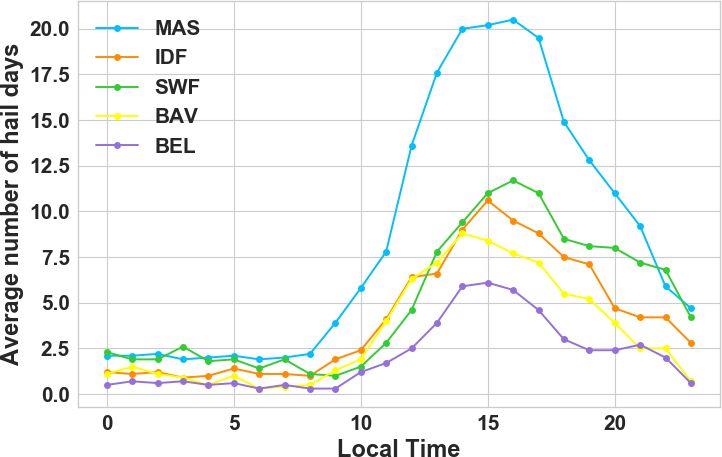
E. Fluck et al.: Radar-based assessment of hail frequency in Europe                                                                 689

and their respective areas are compared (Handwerker, 2002).           by assessing the presence of hail using ESWD reports in the
A split is defined when a cell at time t can be associated with       vicinity of SCS tracks. Out of 26 012 SCS events in total,
two cells at time t + δt. In this case the largest child cell in-     only 985 events could be confirmed by hail reports. The main
herits the history of the parent cell. Similarly, a merger is         reason for this significant reduction of confirmed hail events
defined when two cells at time t are associated with a single         is that ESWD reports are by far not complete. Whereas most
cell at time t +δt. In this case, the largest parent cell assigns a   of the reports are available for Germany, there are far fewer
history to the child cell. The maximum distance between two           hail reports in France, Belgium and Luxembourg.
RC centers that could merge is set to 10 km. Initial and suc-
cessor areas are then compared and the successor is placed
at the weighted center of all initially detected cores. Merging       4     Results
occurs when the successor area is larger than the initial RC.
To avoid reflectivity core crossings or overlapping, each RC          4.1    Spatial distribution of hail
is enumerated and recorded separately.
   After the construction of entire cell tracks, the composite        Figure 3 presents the hail probability map for the radar do-
of maximum reflectivity on a given day does not provide a             main (cf. Fig. 2) in terms of annual average hail days per
smooth result but a rather scattered product. This effect is          year during the period from 2005 to 2014 with a resolution of
most pronounced when the cells propagate further than their           1 × 1 km2 based on 2D radar reflectivity. A day is considered
horizontal extent during a measuring interval. The faster the         a hail day when the threshold of 55 dBZ is exceeded in the
storms move, the more scattered is the maximum reflectivity           daily maximum reflectivity composite after (i) data correc-
projected on a 2D plane. This can substantially reduce reflec-        tion, (ii) filtering with lightning data and (iii) tracking with
tivity values between two scans even though a high-intensity          the object-oriented algorithm CCTA2D as described in the
storm crossed the area. A gap of reflectivity values can also         previous section. If the hail criterion of Z ≥ 55 dBZ is ful-
appear on radar scans in regions with overlapping radar data,         filled on a specific day at a single grid point, this grid point is
especially on neighboring countries such as in the Rhine val-         set to 1, otherwise it is counted as zero. The total of all days
ley. To consider this effect, an advection correction was per-        with hail over the entire 10 year period divided by the num-
formed following Puskeiler et al. (2016). A translation of the        ber of years yields the radar-based “hail climatology”. In ac-
reflectivity cores is computed from one time step to the next         cordance with other hail frequency analyses (e.g., Puskeiler,
considering the horizontal wind field estimated by CCTA2D             2013; Nisi et al., 2016, 2018; Junghänel et al., 2016), the
along a track. The field of motion vectors are computed and           term climatology is used here even though our investigation
projected on the German and French grid. Each point along             refers to a period far below a climatological time scale of
a track includes a velocity shift vector in north-to-south dv         ≥ 30 years. Note that this climatology represents the spatial
and west-to-east du directions. The so-called shift vector U          distribution of convective cells with high reflectivity but not
is denoted as                                                         directly of hail as the 55 dBZ threshold does not guarantee
−
→
                                                                    hail on the ground. Similarly, the absence of high reflectivity
               du(x, y)
U (x, y) =                 .                                    (2)   does not ensure that hail did not occur (see Sect. 3.3). The
               dv(x, y)
                                                                      term hail days used in the following parts of this study refers
   A method is applied to obtain smoothed reflectivity values         to the exceedance of reflectivity but not to confirmed hail ob-
along the tracks detected by the algorithm CCTA2D. First,             servations.
a cluster or “cell” of reflectivity values is detected along the          As can be seen in Fig. 3, the spatial variability of hail days
track at a time t. This cell includes the maximum reflectivity        per year is very large, but some patterns with distinct min-
value at time t as well as its 40 km by 40 km surroundings            ima or maxima can be identified. The lowest number of hail
reflectivity values. After that, the cell is displaced along the      days per year is around the both the Atlantic and the Mediter-
track with a radius of 3 km (Puskeiler, 2013). Then, the first        ranean, with low frequency over northwestern France, Bel-
cell of reflectivity values is shifted forward in time and the        gium and northern Germany. Conversely, the highest number
second cell of reflectivity values is shifted backward in time.       of hail days per year is located towards the east of France,
After that, reflectivity values inside both cells are averaged.       with maxima present in contiguous area such as in central
This procedure is done for multiple intermediate time steps           France (area MAS) or in southwestern Germany. Besides the
in order to create a smooth track.                                    recognizable structures of maxima and minima, some very
   In our analysis, long-living SCS tracks were compared              patchy patterns appear, for example, in area ECG or LUX. As
with hail reports archived by the European Severe Weather             a result, an increasing gradient in the number of hail days per
Database (ESWD) operated by the European Severe Storms                year can be recognized from northwestern France towards
Laboratory (Dotzek et al., 2009) along the reconstructed              central France; a predominant gradient pointing from north-
storm tracks to assess the reliability of CCTA2D. In fact, in         ern towards southern Germany can also be mentioned.
the recent paper by Kunz et al. (2020), the authors separate              A detailed investigation of the hail hotspots is presented
all SCS events used in this study from the hailstorm events           here. Figure 4 represents the location of the mean hail days

https://doi.org/10.5194/nhess-21-683-2021                                       Nat. Hazards Earth Syst. Sci., 21, 683–701, 2021
690 E. Fluck et al.: Radar-based assessment of hail frequency in Europe Figure 3. Annual radar-derived hail frequencies for 1 × 1 km2 grid points in France, Germany, Belgium and Luxembourg between 2005 and 2014. Squares represent boundaries of subdomains further investigated in this study (see Sect. 4.3 for further details). The subdomains were named as follow: NWG (northwest Germany), NEG (northeast Germany), BEL (Belgium), WCG (west central Germany), ECG (east central Germany), NWF (northwest France), IDF (Île-de-France), LUX (Luxembourg), BAV (Bavaria), WCF (west central France), MAS (Massif Central), SWF (southwest France), MED (Mediterranean). Special emphasis is given for subdomains written in red. per year in the Massif Central region overlaid with the 10 m mean wind during hail days from 2005 to 2014 on the high- resolution global relief ETOPO1 having a 1 arc minute reso- lution (Amante and Eakins, 2009). The 10 m mean wind was computed using the hourly and 0.25◦ horizontal resolution ERA5 global analysis (Hersbach et al., 2020). The area with the highest average number of hail days per year during the 10 year investigation period is situated on the leeward side of the highest mountains of the Massif Central, averaging up to 4.6 hail days per year. This maximum ex- tends over the central part over a few kilometers of the Massif Central (Livradois region) composed of a plain and middle- range mountains measuring up to 1300 m high (Livradois mountains). During days with hail, a strong flow comes from the Mediterranean Sea with a southerly direction, thus im- pinging the southern and southeastern mountains of the Mas- sif Central at a sharp angle. Another general westerly flow reaches the western part of the Massif Central. Interestingly, it seems that not only the location of the Massif Central is responsible for the increased number of hail days down- stream, but also the flow convergence where the westerly flow meets with the flow coming from the Mediterranean. Figure 4. Contours of the average number of hail days per year from One may speculate that even without the Massif Central, hail 2005 to 2014 overlaid with the orography and the 10 m mean wind days might be increased in that area of low-level flow con- flow during hail days. vergence. The large valleys on the western side of the Mas- sif Central, oriented from southwest to northeast, facilitate Nat. Hazards Earth Syst. Sci., 21, 683–701, 2021 https://doi.org/10.5194/nhess-21-683-2021
E. Fluck et al.: Radar-based assessment of hail frequency in Europe                                                            691

the passage of the flow coming from the southwest into the         however, this is still a hypothesis that requires additional ob-
Livradois region. This region, with an average number of           servations and numerical simulations in this region to assess
3.2 hail days per year, is located in an area where the wind       convection initiation.
vectors converge both in the direction and velocity. In order         The northeastern part of France, including the regions of
to better understand the flow characteristics over the Massif      Burgundy (region 9 in Fig. 1), Champagne-Ardenne (region
Central shown in Fig. 4, we calculated the Froude number on        6), Alsace (region 8), Lorraine (region 7) and Franche-Comté
radar-derived hail days from ERA5 (Queney, 1948; Smith,            (region 10) are affected with a maximum of 3.1 hail days per
1979) for a region covering the Massif Central entirely and        year in the central part of Burgundy and more precisely on
ranging from 44.0 to 46.5◦ N and from 2.0 to 4.7◦ E. The           the eastern side of mountains ranging from approximately
Froude number is calculated as follows:                            300 to 900 m. In Champagne-Ardenne the number of hail
        U                                                          days per year reaches up to 2.9 d over the mainly rolling ter-
Fr =      ,                                                 (3)    rain. In Lorraine, where the terrain is almost flat and the cli-
       NH
                                                                   mate is more continental, an average of 2.7 hail days per year
where U represents the wind speed perpendicular to the             were counted in its central part. A local and lower maximum
mountain and was computed by applying a density-weighted           of 2.4 hail days per year can be recognized in South Alsace,
integration over the lowest 2000 m. H is a characteristic          representing an area with complex terrain with mountains up
mountain height set to 1300 m for the Massif Central region        to 1424 m a.g.l.
and N is the Brunt–Väisälä frequency. The Brunt–Väisälä               Another hail hotspot in the northeastern part of France is
frequency, N, is defined as                                        found along the northern ridge of the Jura Mountains (la-
     s                                                             beled E in Fig. 1) in Franche-Comté with 2.5 hail days per
         g ∂θv                                                     year. Note that the Jura mountains represent a natural ob-
N=             ,                                        (4)
        θv ∂z                                                      stacle frequently triggering thunderstorms (Piper and Kunz,
                                                                   2017) and hailstorms by orographical lifting (e.g., Langhans
where g is the gravitational acceleration equal to 9.8 m s−2 ,     et al., 2013; Schemm et al., 2016; Nisi et al., 2018).
θv is the virtual potential temperature and ∂θ  v
                                              ∂z represents the       The Rhône-Alpes (region 11 in Fig. 1) is a region like-
vertical gradient of the virtual potential temperature. In our     wise frequently affected by hail. This region contains the
analysis, we considered the root mean square of the Brunt–         large Rhône valley and is bordered by the Massif Central
Väisälä frequency, N, in order to exclude imaginary values.        in the west and by the Alps to the east. The southwestern
   The mean Froude number on hail days over the Massif             part as well as the southeastern edge of the region show a
Central from 2005 to 2014 is Fr = 0.39 ± 0.3. According            local hail maximum with up to 3.1 hail days per year. The
to Smith (1979) and Smolarkiewicz and Rotunno (1989), a            existence of these two hotspots may be explained by their
Froude number below 1 suggests a flow that goes around the         proximity to the Mediterranean as, during southerly flows,
mountain rather than directly over it. Thus, it can be assumed     warm and moist air is advected preferably through the Rhône
that the flow around the Massif Central is deviated by the         valley. The warm and moist air can then be lifted, for exam-
mountain peaks leading to convergence downstream at low            ple, near a front system crossing the country from northwest
levels on the leeward side of the Massif Central where the         to southeast, leading to forced convection. This effect was
hail hotspot is located. This deflection of the flow is unlikely   confirmed by Schemm et al. (2016), who analyzed the re-
to show up in Fig. 4 due to the fairly coarse resolution of the    lation between radar-based hailstreaks over Switzerland and
ERA5 reanalysis.                                                   adjacent regions and cold fronts identified in high-resolution
   Several authors have found an increased hail frequency          model data (COSMO-2; Steppeler et al., 2003; Jenkner et al.,
downstream rather than upstream or directly above the moun-        2010) during a 12 year period (2002 to 2013). The authors
tains. This is, for example, the case in the Pyrenean region       found that around 45 % of the detected hail cell initiations
(Vinet, 2001; Berthet et al., 2011; Hermida et al., 2013;          located on the windward side of the pre-Alps (in the Rhône
Merino et al., 2013) near the Black Forest in Germany (Kunz        valley) are associated with cold fronts coming from the west
and Puskeiler, 2010; Puskeiler et al., 2016) and in the vicinity   during the summer months (May to September).
of the Alps (Eccel et al., 2012; Nisi et al., 2018). By refer-        Southwestern France, including both the Aquitaine and
ring to the studies by Mass (1981) about leeward side con-         Midi-Pyrenees regions (regions 12 and 13 in Fig. 1), is also
vergence near the Olympic mountains in Washington State            frequently affected by hail with up to 2.6 hail days per year
and by Barthlott et al. (2016) on convection initiation near       in the southwest range of the Massif Central. The Aquitaine
the Corsica mountains during HyMeX (Hydrological cycle             and Midi-Pyrenees regions are the two regions well known
in the Mediterranean eXperiment), Kirshbaum et al. (2018)          in the literature for their high hail probability (Vinet, 2001;
found that leeward side convergence produces the ascent re-        Punge et al., 2014). Hermida et al. (2015) used data from the
quired for convective initiation on the leeward side of moun-      ANELFA (Association Nationale d’Etude et de Lutte con-
tains. Low-level flow convergence could explain the high fre-      tre les Fléaux Atmosphériques) hailpad network and found
quency of hail on the leeward side of the Massif Central;          that the Gers department, located on the west side of the

https://doi.org/10.5194/nhess-21-683-2021                                   Nat. Hazards Earth Syst. Sci., 21, 683–701, 2021
692 E. Fluck et al.: Radar-based assessment of hail frequency in Europe Midi-Pyrenees region, is the area the most affected by hail The northwestern part of Germany, including the states of in southwestern France. The western and northern sides of Hesse (region 2 in Fig. 1) and Rhineland-Palatinate (region 3 the Pyrenees are also frequently affected by hail with up to in Fig. 1), and the southern part of North Rhine-Westphalia 2.5 hail days per year. According to Berthet et al. (2011), hail (region 1 in Fig. 1) are regions affected by approximately in that region frequently occurs when a low-pressure system 1.4 hail days per year on average. The location of the hail is located over the western part of Spain leading to south- patterns show an association with the local orography with a westerly flow over France associated with the advection of pronounced maximum in north Hesse that lies directly on the warm and moist air over the Pyrenean mountain range. leeward side of the Westerwald low mountain range, which In Germany, the main hail hotspot is located in the south- is characterized by rolling terrain. west in the federal state of Baden-Württemberg (region 4 in Fig. 1), specifically over the Swabian Jura (B in Fig. 1), south 4.2 Annual variability of the city of Stuttgart, with a maximum of 3.1 hail days per year. This hotspot has already been identified in previ- The frequency of SCSs shows a very large annual and mul- ous studies by Puskeiler (2013) and Junghänel et al. (2016). tiannual variability (e.g., Nisi et al., 2018). This variabil- Using Eq. (3), we found a Froude number of Fr = 0.51 ± 0.6 ity is partly related to large-scale flow mechanisms such as for 207 hail days during the period 2005 to 2014 for a re- the presence of specific Northern Hemisphere teleconnection gion covering 48 to 49.2◦ N and 7.8 to 10.5◦ E, including patterns representing the low-frequency mode of the climate the Swabian Jura as well as the Black Forest and consid- system (e.g., North Atlantic Oscillation (NAO) or East At- ering a maximum elevation of 1400 m for the entire area. lantic (EA) pattern) or by variations in the sea surface tem- The Froude number found in our study in the southwestern perature (Piper et al., 2019). Having reconstructed a very part of Germany matches the results of Kunz and Puskeiler large event set of SCSs/hailstorms, as presented in the pre- (2010) who estimated a Froude number for a region cover- vious section, we are also interested in how the frequency of ing the Vosges mountains, the Rhine valley, the Black For- these events vary across the whole domain and regionally. est and the Swabian Jura of Fr = 0.32 ± 0.15 for 65 hail Averaged over the entire investigation area, the annual days (1997–2007) using radiosondes at 12:00 UTC. This low number of hail days is between 72 (2010) and 103 (2006) Froude number suggests a flow-around regime of the south- with a mean of 86 (Fig. 5). In 2006, large parts of Eu- ern and northern mountains of the Black Forest causing a rope, including Germany, Belgium, Luxembourg and north- zone of horizontal flow convergence downstream. This con- west France, experienced higher temperatures than on av- vergence zone coincides with the area of the highest num- erage, especially during the end of June and July (NOAA, ber of hail days (Kunz and Puskeiler, 2010; Koebele, 2014). 2007), when two (moderate) heat waves occurred (Fouillet Moreover, Kunz and Puskeiler (2010) hypothesized that the et al., 2008). As a result, the sea surface temperature over southwesterly flow meets the Swabian Jura at a very sharp the Mediterranean showed a positive anomaly (NOAA, 2007; angle, which reduces the Froude number considerably and Lenderink et al., 2009), leading to intense evaporation rates aligns the wind parallel to the mountain chain. This flow and, consequently, to an increase in the amount of water va- modification is assumed to be responsible for the flow con- por in the atmosphere (Chaboureau et al., 1998). The spatial vergence at low levels as was also found in model simulations distribution of hail days in 2006 (Fig. 6) strongly resembles using COSMO-DE by Koebele (2014). the climatology, with several maxima near hilly terrains and Another local maximum of up to 2.6 hail days per year is minima near the coastlines. Some hotspots can also be de- found north of the Alps, on the western part of the State of tected over the northwest part of France and in southwestern Bavaria (region 5 in Fig. 1). This result is in good agreement Germany. with the conclusion of Nisi et al. (2018) who found that this Even though the year of 2010, showing the lowest num- region can be affected by around 3 hail days per year (2002– ber of hail days, was very warm on the global scale (NOAA, 2014). 2011), summer temperatures over large parts of Europe in- In the northeast of Germany, a local maximum of up to 3.2 cluding Germany were below average. Furthermore, sev- hail days per year is positioned over the Saxon Ore Moun- eral persistent large-scale ridges occurred during the sum- tains (labeled A in Fig. 1) south of the city of Dresden. Note, mer, which may have suppressed the formation of SCSs however, that this maximum is mainly caused by a high num- (DeutscheRück, 2013). No clear spatial pattern can be found ber of SCSs in the year of 2007 (Piper, 2017), which was in this year with only a few hailstorms in central France. Al- characterized by frequent upper air troughs over western Eu- most no hailstorms could be detected in an arc spanning from rope and ridges over central Europe (Wernli et al., 2010), northwestern France to northern Germany. There are further leading to high-pressure gradients on the eastern part of regions where hail was less present compared to the mean of Germany in combination with a southeast-to-northeast flow 2010, including all of Belgium, Luxembourg and the north- regime from Czechia (note that the almost same situation oc- west of France, especially Normandy, Brittany and the coast- curred in 2019). lines. Nat. Hazards Earth Syst. Sci., 21, 683–701, 2021 https://doi.org/10.5194/nhess-21-683-2021
E. Fluck et al.: Radar-based assessment of hail frequency in Europe                                                           693

                                                                       The mountainous subdomain MAS shows the largest aver-
                                                                    age number of hail days and has the most pronounced annual
                                                                    cycle. Until the end of April, the average number of hail days
                                                                    for the 10 d running mean is below 10. During May and the
                                                                    beginning of June, the number increases substantially from
                                                                    9 d around 5 May up to 17 d on 4 June. The more pronounced
                                                                    diurnal temperature cycle for continental regions, associated
                                                                    with a higher lapse rate in combination with orographic lift-
                                                                    ing, may explain this increase (Berthet et al., 2011). After
                                                                    4 June, the average number of hail days increases steadily
                                                                    until reaching the overall maximum for the MAS region at
                                                                    the end of July with 23 d.
                                                                       Likewise, subdomain IDF shows a high hail frequency
                                                                    during the summer with up to 14 d, mainly at the end of July.
                                                                    This subdomain is under the influence of the Atlantic Ocean
Figure 5. Yearly number of hail days per year from 2005 to 2014.
The red line indicates the overall mean of hail days from 2005 to
                                                                    (Cantat, 2004), leading to an increased frequency of troughs
2014.                                                               (Vinet, 2001, Berthet et al., 2013).
                                                                       Within this subdomain, the number of hail days increases
                                                                    slightly until the peak with a first local maximum in the
4.3   Seasonal and diurnal development of SCSs                      beginning of June (around 10 hail days) and a second lo-
                                                                    cal maximum at the beginning of July with around 12 hail
The large spatiotemporal variability of hail discussed in the       days. Spring hailstorms may be associated with subtropical
previous sections leads us to the question of the seasonal          air masses coming from Spain, while summer storms prefer-
and diurnal development of SCSs at the regional level. For          ably form ahead of cold fronts (Berthet et al., 2011). The
this purpose, the entire study area is divided into 13 subdo-       number of hail days decreases sharply from the hail peak sea-
mains of similar size (around 75 000 km2 ) framed in Fig. 3.        son toward the end of September.
We selected five subdomains with different terrain and cli-            Subdomain SWF has a very broad hail peak in the middle
matological characteristics for further discussion: Belgium         of June with 12 hail days centered around 14 June. After-
(BEL), Ile-de-France (northern France; IDF), Bavaria (south-        wards, the number slightly decreases and reaches 4 hail days
eastern Germany, BAV), the Massif Central (central France;          at the end of September. This maximum found in June dif-
MAS) and southwest France (SWF). Subdomains BEL, SWF                fers from the analysis of Dessens et al. (2015), who found
and IDF have a climate strongly influenced by maritime air          that May is the most active month followed by July over the
masses. Among them, subdomains BEL and IDF represent                southwestern part of France and the Mediterranean area (sit-
flatlands, while subdomain SWF contains the high moun-              uated along the Rhône valley). Also, Fraile et al. (2003) and
tains of the Pyrenees. Subdomains BAV and MAS both have             Hermida et al. (2013) found that May is the month with the
a rather continental climate but have a different orography.        highest hail kinetic energy in southwestern France. Reasons
While mainly hilly terrain characterizes subdomain BAV,             for this discrepancy can be due to a longer period analyzed by
subdomain MAS comprises the higher mountains of the Mas-            Dessens et al. (2015), while Hermida et al. (2013) and Fraile
sif Central.                                                        et al. (2003) focused on a time range starting from the 1990s.
   To quantify the number of hail days in each subdomain,              Subdomain BAV, located in southeast Germany, has the
the average number of hail days for consecutive 10 d periods        maximum number of hail days at the end of July, later in the
was calculated for the period 2005 to 2014 (Fig. 7). Despite        year than the other subdomains. Kunz and Puskeiler (2010)
the large variability seen in the seasonal cycles of the subdo-     and Puskeiler (2013) also found that July is the month with
mains considered, some similarities can be recognized. All          the highest number of hail days in central and southern Ger-
time series of the different subdomains feature a clear annual      many.
cycle with a minimum number of hail days in spring and                 Subdomain BEL, covering the north of France as well as
autumn and a maximum number during the summer. This                 much of Belgium, peaks at the end of June. A 10 year radar-
characteristic cycle with a strong increase in the hail day         based climatology conducted for Belgium by Lukach and
frequency during April/May, a significant decrease around           Delobbe (2013) also found that May and June are the most
September and a maximum during the summer months was                favorable months for hail.
found by several other authors such as Dessens (1986) and              The development of hailstorms shown in Fig. 8 represents
Vinet (2002) for France, Belgium and Luxembourg, Gudd               the times where the CCTA2D detects the first radar reflec-
(2003), Deepen (2006), Mohr and Kunz (2013) and Puskeiler           tivity of 55 dBZ or more. Since the local time (LT) varies
et al. (2016) for Germany and Nisi et al. (2014, 2018) for          through Europe by approximately 1 h from Brittany in France
Switzerland and northern Italy.                                     to Saxony in Germany, all times originally given in UTC are

https://doi.org/10.5194/nhess-21-683-2021                                    Nat. Hazards Earth Syst. Sci., 21, 683–701, 2021
694 E. Fluck et al.: Radar-based assessment of hail frequency in Europe
Figure 6. Number of radar-derived hail days shown for the years with the highest (2006, left) and lowest (2010, right) hail day frequency.
Figure 7. Time-series of the mean number of radar-derived hail Figure 8. Hourly distribution of the mean number of radar-derived
days for consecutive 10 d periods for the subdomains BEL, IDF, hail days for each subdomain.
BAV, MAS and SWF shown in Fig. 3.
due to local orographic effects, such as slope or valley winds
converted to LT, representing 4 min per degree of longitude. (Nesbitt and Zipser, 2003).
In all subdomains, hail occurs most frequently in the after- For subdomain SWF, the average number of hail days re-
noon between 13:00 and 18:00 LT, while between midnight mains high in the late evening (20:00 to 22:00 LT).
and 10:00 LT the fewest events are detected (Fig. 8). A plausible effect is that severe storms may develop from
Some discrepancies appear in the daily cycle, mainly de- pre-existing scattered thunderstorms that form during the af-
pending on the location and characteristics of the respec- ternoon as was found by Nisi et al. (2016, 2018). This feature
tive subdomain. For example, the frequency of hailstorms in might be decisive for the hailstorm maximum in the evening
BEL reveals a large increase during the afternoon (14:00– in the canton of Ticino in southern Switzerland.
15:00 LT) and a slow but gradual decrease toward the morn- Some literature exists regarding the diurnal cycle of hail
ing. in Europe (Punge and Kunz, 2016). Bedka (2011), for exam-
In contrast to the subdomains located in the northern part ple, recognized a diurnal cycle of overshooting tops that is
of Europe, domains MAS over the Massif Central and SWF related to the presence of orography and/or to the distance to
slightly peak 1 h later at around 16:00 LT. The peak during the sea. Kaltenböck et al. (2009) found a peak in hail occur-
the late afternoon for more continental regions is presumably rence in the middle of the afternoon through Europe. Kunz
Nat. Hazards Earth Syst. Sci., 21, 683–701, 2021 https://doi.org/10.5194/nhess-21-683-2021You can also read