Towards an efficient storm surge and inundation forecasting system over the Bengal delta: chasing the Supercyclone Amphan - Natural Hazards and ...
←
→
Page content transcription
If your browser does not render page correctly, please read the page content below
Nat. Hazards Earth Syst. Sci., 21, 2523–2541, 2021
https://doi.org/10.5194/nhess-21-2523-2021
© Author(s) 2021. This work is distributed under
the Creative Commons Attribution 4.0 License.

Towards an efficient storm surge and inundation forecasting system
over the Bengal delta: chasing the Supercyclone Amphan
Md. Jamal Uddin Khan1 , Fabien Durand1,2 , Xavier Bertin3 , Laurent Testut1,3 , Yann Krien3,a , A. K. M. Saiful Islam4 ,
Marc Pezerat3 , and Sazzad Hossain5,6
1 LEGOS     UMR5566, CNRS/CNES/IRD/UPS, 31400 Toulouse, France
2 Laboratório   de Geoquímica, Instituto de Geociencias, Universidade de Brasilia, Brasília, Brazil
3 UMR 7266 LIENSs, CNRS – La Rochelle University, 17000 La Rochelle, France
4 Institute of Water and Flood Management (IWFM), Bangladesh University of Engineering and Technology (BUET),

Dhaka-1000, Bangladesh
5 Flood Forecasting and Warning Centre, BWDB, Dhaka, Bangladesh
6 Department of Geography and Environmental Science, University of Reading, Reading, UK
a currently at: SHOM (DOPS/STM/REC), Toulouse, France

Correspondence: Md. Jamal Uddin Khan (jamal.khan@legos.obs-mip.fr)

Received: 14 October 2020 – Discussion started: 30 October 2020
Revised: 15 March 2021 – Accepted: 17 June 2021 – Published: 25 August 2021

Abstract. The Bay of Bengal is a well-known breeding              1   Introduction
ground to some of the deadliest cyclones in history. Despite
recent advancements, the complex morphology and hydro-
dynamics of this large delta and the associated modelling         Storm surges and associated coastal flooding are one of the
complexity impede accurate storm surge forecasting in this        most dangerous natural hazards along the world coastlines.
highly vulnerable region. Here we present a proof of con-         Annually, storm surges have killed on average over 8000 peo-
cept of a physically consistent and computationally efficient     ple and affected 1.5 million people worldwide over the past
storm surge forecasting system tractable in real time with        century (Bouwer and Jonkman, 2018). Among the storm-
limited resources. With a state-of-the-art wave-coupled hy-       surge-prone basins, the Bay of Bengal in the northern In-
drodynamic numerical modelling system, we forecast the            dian Ocean is one of the deadliest. This basin has consis-
recent Supercyclone Amphan in real time. From the avail-          tently been home to the world’s highest surges, experiencing
able observations, we assessed the quality of our modelling       in each decade an average of five surge events exceeding 5 m
framework. We affirmed the evidence of the key ingredients        (Needham et al., 2015). On 18 May 2020, a supercyclone
needed for an efficient, real-time surge and inundation fore-     named Amphan was identified as the most powerful ever
cast along this active and complex coastal region. This article   recorded in the Bay of Bengal, with the highest sustained
shows the proof of the maturity of our framework for oper-        3 min wind speed exceeding 240 km/h (130 knots) and the
ational implementation, which can particularly improve the        highest 1 min wind gusts reaching 260 km/h (https://www.
quality of localized forecast for effective decision-making       metoc.navy.mil/jtwc/jtwc.html, last access: 30 May 2020).
over the Bengal delta shorelines as well as over other sim-       On 20 May, 2 d later, Amphan made landfall in West Bengal
ilar cyclone-prone regions.                                       (India), with a sustained wind speed of 112 km/h and gusts of
                                                                  190 km/h, causing massive damage in India and Bangladesh
                                                                  and claiming at least 116 lives (IFRC, 2020a, b).
                                                                     The cyclone activity in the Bay of Bengal is very dif-
                                                                  ferent from the other cyclone-prone oceanic basins (Need-
                                                                  ham et al., 2015). The basin experiences a distinct bi-modal
                                                                  distribution of cyclonic activity – one with a peak in the

Published by Copernicus Publications on behalf of the European Geosciences Union.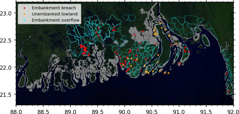
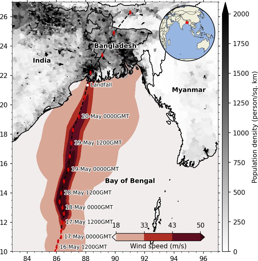
2524                                                               M. J. U. Khan et al.: Chasing the Supercyclone Amphan

pre-monsoon (April–May) and another during post-monsoon
(October–November) (Bhardwaj and Singh, 2019). The Bay
of Bengal is a small semi-enclosed basin (Fig. 1) which ac-
counts for only 6 % of cyclones worldwide. However, more
than 70 % of global casualties from the cyclones and associ-
ated storm surges over the last century occurred there (Ali,
1999). The number of fatalities concentrates in the Bengal
delta across Bangladesh and India (Ali, 1999; Murty et al.,
1986), where more than 150 million people live below 5 m
above mean sea level (a.m.s.l.) (Alam and Dominey-Howes,
2014). Seo and Bakkensen (2017) noted a statistically sig-
nificant correlation between storm surge height and the fa-
tality rate in this region. Two of the notable cyclones that
struck this delta include the 1970 Cyclone Bhola and 1991
Cyclone Gorky, which killed about 300 000 (Frank and Hu-
sain, 1971) and 150 000 (Khalil, 1993) people, respectively.
In recent decades, the death toll has reduced by orders of
magnitude. For example, Cyclone Sidr, a Category 5 equiv-
alent cyclone on the Saffir–Simpson scale that made land-
fall in 2007, claimed 3406 lives (Paul, 2009). At the same
time, the cost of material damages has significantly increased
(Alam and Dominey-Howes, 2014; Emanuel, 2005; Schmidt              Figure 1. The path of the Supercyclone Amphan of May 2020, over-
et al., 2009). During recent cyclones, government and vol-         laid on the population density (Center For International Earth Sci-
untary agencies of Bangladesh and India made a coordinated         ence Information Network (CIESIN), Columbia University, 2016).
effort to evacuate millions of people to safety at cyclone shel-   The footprint of 18 m/s (tropical storm), 33 m/s (Category 1), 43 m/s
ters before the cyclone landfall (Paul and Dutt, 2010). This       (Category 2), and 50 m/s (Category 3) wind speed area is shown
kind of informed coordination benefited from improved com-         with the red colour bar (classified as in the Saffir–Simpson scale).
munication; increased shelter infrastructure; and, most im-        Inset shows the location of the study area.
portantly, from the improvement of the numerical prediction
of storm track and intensity.
   Over the last decades, global weather and forecasting sys-      teorological Organization (WMO), the IIT-D model is also
tems have advanced significantly. Several global models now        implemented to run in the Bangladesh Meteorological De-
run multiple times a day, starting from multiple initial condi-    partment (BMD). Beside the IIT-D model, the BMD also
tions, with horizontal resolutions on the order of tens of kilo-   experimentally uses the Meteorological Research Institute
metres, providing forecasts with a range of hours to a week.       (MRI) storm surge model from the Japan Meteorological
These forecasts have proven useful during weather extremes         Agency (JMA) (http://bmd.gov.bd/p/Storm-Surge, last ac-
like tropical storms (Magnusson et al., 2019). Operational         cess: 30 May 2020). Storm surge forecasts have shown their
hurricane forecasting systems like Hurricane Weather Re-           potential to better target the evacuation decision, to optimize
search and Forecasting (HWRF) have emerged and reached a           early-engineering preparations, and to improve the efficiency
level of maturity to provide reliable cyclone forecasts several    of the allocation of the resources (Glahn et al., 2009; Lazo
days in advance throughout the tropics (Tallapragada et al.,       and Waldman, 2011; Munroe et al., 2018). Availability of a
2014).                                                             spatially distributed forecast of storm surge flooding can fur-
   Storm surge forecasting has been developed and imple-           ther increase the fluidity of communication toward the pub-
mented around the world along with the advancement of              lic (Lazo et al., 2015). Keeping in mind the cyclonic surge
the weather and storm forecasting (Bernier and Thompson,           hazards over the densely populated Bengal delta, having a
2015; Daniel et al., 2009; Flowerdew et al., 2012; Lane et al.,    reliable real-time operational forecast system in the region
2009; Verlaan et al., 2005). Nowadays, operational surge           would be extremely valuable and would address a societal
forecasting systems typically run on high-performance com-         demand (Ahsan et al., 2020). The major challenges in op-
puting systems, either on a scheduled basis or triggered on-       erating and maintaining such systems are manifold for the
demand during an event (Loftis et al., 2019; Oliveira et al.,      Bengal delta, including lack of expertise, limitations of fund-
2020; Khalid and Ferreira, 2020). In the Bay of Bengal re-         ing resources to operate and maintain necessary infrastruc-
gion, the Indian Institute of Technology-Delhi (IIT-D) storm       ture and datasets, and availability of reliable modelling sys-
surge model has been running operationally with a horizon-         tems in operational mode (Roy et al., 2015).
tal resolution of 3.7 km for 1 decade (Dube et al., 2009). Un-        Storm surge modelling is, however, computationally ex-
der the Tropical Cyclone Program (TCP) of the World Me-            pensive and has proven to be challenging in real-time-

Nat. Hazards Earth Syst. Sci., 21, 2523–2541, 2021                                  https://doi.org/10.5194/nhess-21-2523-2021
M. J. U. Khan et al.: Chasing the Supercyclone Amphan                                                                        2525

forecasting mode (Glahn et al., 2009; Murty et al., 2017).            Cyclone Amphan is not only the latest event on record in
Several practical solutions exist to curb the real-time con-       the Bay of Bengal but also the costliest event that struck
straints of cyclone forecasts, such as soft real-time compu-       this shoreline, with an estimated bill of over USD 14 bil-
tation based on looking up an extensive database of pre-           lion in West Bengal and Bangladesh (DhakaTribune, 2020;
computed cyclones (Condon et al., 2013; Yang et al., 2020),        IFRC, 2020a). During this cyclone, we have proactively fore-
coarse-resolution modelling (Suh et al., 2015), and mod-           cast storm surge in real time with common computational
elling without wave-coupling (Murty et al., 2017). Over the        resources using a high-resolution coupled modelling system
past decades, unstructured-grid modelling systems are get-         forced by a combination of freely available atmospheric fore-
ting more and more popular due to their efficiency in resolv-      casts. The general goal of this paper is to provide a proof
ing the topographic features and their reduced computational       of concept of a tractable operational storm surge forecasting
cost compared to structured-grid equivalents (Ji et al., 2009;     system over this key region of vulnerability, to identify the
Lane et al., 2009; Melton et al., 2009; Fortunato et al., 2017;    key ingredients of such a system, and to provide guidance in
Khalid and Ferreira, 2020).                                        the near-future initiatives of the operational forecasting com-
   The published history of storm surge modelling in the           munity. First, we present the various processes governing
northern Bay of Bengal goes hand in hand with the land-            the surge dynamics to illustrate the challenges of modelling
falling of very severe cyclones (Das, 1972; Flather, 1994;         storm surges in the Bay of Bengal in Sect. 2. Section 3 docu-
Dube et al., 2004; Murty et al., 2014; Krien et al., 2017).        ments the atmospheric forecasts that are required to generate
From the modelling of the historical storm events, previous        a surge forecast. In Sect. 4, we introduce our numerically effi-
studies have identified several ingredients as essential for ac-   cient hydrodynamics–waves coupled modelling platform and
curate modelling and forecasting of storm-surge-induced wa-        present its practical real-time computational set-up in Sect. 5.
ter level and associated flooding over the Bengal delta. The       Finally, we present the remaining modelling and forecast-
most important of these ingredients is an accurate bathymetry      ing issues in Sect. 6. Section 7 provides a conclusion to this
and topography (Krien et al., 2016, 2017; Murty et al., 1986).     study.
Second, it is required to have a large-scale modelling do-
main comprising the whole Ganges–Brahmaputra–Meghna
(GBM) estuarine network (Johns and Ali, 1980; Oliveira             2   Storm surge and inundation processes in the Bay of
et al., 2020) at a high-enough model resolution (Krien et al.,         Bengal
2017; Kuroda et al., 2010). The modelling framework is re-
quired to simulate tide and surge together to account for the      The Bay of Bengal is a macro-tidal region where peak tidal
tide–surge interactions (As-Salek and Yasuda, 2001; Johns          range reaches as high as 5 m over the north-eastern corner of
and Ali, 1980; Kuroda et al., 2010; Murty et al., 1986). Fur-      the bay (Krien et al., 2016; Tazkia et al., 2017). A large ge-
thermore, an online coupling of the hydrodynamics and the          ographical extent of the land–sea hydraulic continuum with
short waves is also necessary to account for the wave set-up       an intricate estuarine network complicates the water level dy-
(Deb and Ferreira, 2016; Krien et al., 2017). The capability       namics in this part of the coastal ocean. During a cyclone, the
of the model to simulate the wetting and drying is also neces-     dynamics get even more complicated due to wave-induced
sary to model the inundation (Madsen and Jakobsen, 2004).          set-up and tide–surge interaction. In Fig. 2, we illustrate a
   Fully coupled tide–surge–wave models have been recom-           simplified view of water level components – tide, surge, wave
mended for operational forecasting in the Bay of Bengal for        set-up – and their interactions with the topography in driving
years (Johns and Ali, 1980; Murty et al., 1986; As-Salek           inundation during a cyclone.
and Yasuda, 2001; Deb and Ferreira, 2016; Krien et al.,               During a cyclone, the atmospheric pressure drop and the
2017). Besides the development of the wave–ocean cou-              wind stress both generate the water level surge. This atmo-
pled hydrodynamic modelling tool itself, the main challenge        spheric storm surge is non-linearly dependent on the astro-
in implementing such a system is due to the high com-              nomical tide. The dependent nature of both tide and surge
putational requirements for the modelling systems (Murty           implies that the surge induced by a given meteorological
et al., 2014, 2016). Due to these constraints, operational sys-    condition differs at different stages of the tide, particularly
tems are commonly run with either only a surge or cou-             in the nearshore shallow zone. This departure from linearly
pled tide–surge model at kilometric resolution (Dube et al.,       added tide and surge component is known as tide–surge in-
2009). In recent years, higher resolution (100 m at the coast)     teraction. In a macro-tidal region like the Bengal delta, tide–
unstructured-grid models have been used for operational            surge interaction typically amounts to several tens of cen-
forecasts over part of Indian coastlines in the Bay of Bengal      timetres (Antony and Unnikrishnan, 2013; Idier et al., 2019).
but without wave-coupling (Murty et al., 2017). These limita-      Due to this interaction, the highest surge (water level – tide)
tions in operational forecasting systems can significantly im-     does not coincide with high tide as shown from observations
pede a proper interpretation during an actual cyclonic storm,      (Antony and Unnikrishnan, 2013) and numerical modelling
as discussed in the next section through a set of hindcast sen-    (Krien et al., 2017; Antony et al., 2020). The strong depen-
sitivity experiments of Cyclone Amphan.                            dence on tide reinforces the importance of having an accu-

https://doi.org/10.5194/nhess-21-2523-2021                                Nat. Hazards Earth Syst. Sci., 21, 2523–2541, 2021
2526                                                              M. J. U. Khan et al.: Chasing the Supercyclone Amphan

rate tidal model for the region and a reliable network of wa-     around 18:00 UTC, the maximum wind speed increased from
ter level gauge for validation (As-Salek and Yasuda, 2001;        140 to 215 km/h, making it an extremely severe cyclonic
Krien et al., 2017; Kumar et al., 2015; Murty et al., 2016).      storm (equivalent to Category 4 on the Saffir–Simpson scale).
   Wave set-up is another component that has a significant        Over the next 12 h, Amphan continued to intensify, reaching
impact on the nearshore sea level (Idier et al., 2019; Krien      a maximum of 260 km/h wind speed and 907 mbar central
et al., 2017; Murty et al., 2014). It manifests as an increase    pressure, making it the most intense event on record in the
in the sea level occurring in the nearshore zone that accom-      Bay of Bengal. During this time, it appeared to form two dis-
panies the dissipation of short waves by breaking (Longuet-       tinct eye walls, which is typical of intense cyclones. Over
Higgins and Stewart, 1962). During Cyclone Sidr, the mod-         the next 24 h, Amphan lost most of its strength due to the
elled wave set-up was around 30 cm (Krien et al., 2017).          eye wall replacement cycle in the presence of moderate ver-
This estimation would be potentially underestimated by up to      tical wind shear (30–40 km/h). The system continued to de-
100 % due to an early dissipation of wave energy by depth-        cay due to easterly shear and mid-level dry air. The vertical
induced breaking arising from usual parameterizations uti-        wind shear remained moderate during this period. The cy-
lized in spectral wave models (Pezerat et al., 2020, 2021).       clone made landfall between 08:00 and 10:00 UTC around
   At the seasonal scale, the mean sea level around the Ben-      88.35◦ N, 21.65◦ E (Fig. 1), at mid-tide. At landfall, the re-
gal delta also shows considerable evolution. The amplitude        ported central pressure amounted to 965 mbar, with a maxi-
of this variation can go as high as 40 cm due to freshwater       mum wind speed of 150–160 km/h. Afterwards, over its jour-
influxes during the monsoon from the GBM river system and         ney inland, the system further eroded and disappeared by 21
offshore-ocean steric variability (Durand et al., 2019; Tazkia    May. The black lines in Fig. 3 illustrate the evolution of Am-
et al., 2017). During the wintertime cyclone-prone season,        phan from the JTWC best track.
this steric variability can induce 10–15 cm variation in mean        The extended range outlook by the IMD published on 7
sea level of the bay.                                             May predicted cyclogenesis to occur between 8 and 14 May
   Except for the Sundarban mangrove forest, coastal              with low probability (IMD, 2021). Global and regional mod-
Bangladesh is mostly embanked through a network of 139            els started to predict that a significant storm would happen in
polders (Nowreen et al., 2013). These embanked areas can be       the Bay of Bengal as early as 12 May, 8 d before the cyclone
flooded in three ways: (a) by overflowing or overtopping, (b)     landfall and 4 d before the actual formation of the tropical
by breaching of the embankments or control structures, and        depression. The formation of the low-pressure system trig-
(c) by heavy rainfall inside the embanked area. The height of     gered the operational HWRF system of the NOAA (https:
these embankments plays the most vital role in actuating the      //www.emc.ncep.noaa.gov/gc_wmb/vxt/HWRF/, last access:
inundation from a storm surge (Krien et al., 2017). The per-      30 May 2020) on 14 May. Similarly, the operational system
formance of the embankments during the cyclone is another         of the IMD (https://nwp.imd.gov.in/hwrf/IMDHWRFv3.6)
crucial factor, depending on the composition (typically, earth    was also triggered a day later. For the rest of the paper,
vs. stones or concrete). During a cyclone, the wave action        we confine our analysis to the forecast disseminated by the
as well as overtopping and overflowing on the embankments         NOAA-HWRF only, relying on the Automated Tropical Cy-
can create breaches at a weak point, thus creating local inland   clone Forecasting System (ATCF) text output (Miller et al.,
flooding (Islam et al., 2011). Particularly for Bangladesh,       1990). Figure 3 illustrates a few of the selected forecast cy-
the consequence of such storm-surge-induced flooding can          clone tracks sequentially issued from the NOAA-HWRF.
be long-lasting as the topography inside polders is often be-        The forecasts illustrate the convergence of the location of
low the mean sea level due to ground compaction (Auerbach         the landfall. As early as 17 May, 3 d before the landfall, the
et al., 2015).                                                    forecast tracks had converged towards the observed track. On
                                                                  18 May, 1 d later, the forecast error in the storm track loca-
                                                                  tion had reduced to around 50 km. The forecast wind speed
3   Atmospheric evolution of Cyclone Amphan                       and central pressure did not show as much accuracy as the
                                                                  forecast trajectory. The initial forecasts captured the magni-
On 13 May 2020, a low-pressure area was persisting over           tude of the intensification. However, they failed to forecast
the northern Bay of Bengal about 300 km east of Sri Lanka.        the rapid intensification that occurred during 17–18 May. On
By the end of 15 May, the Joint Typhoon Warning Center            the other hand, the subsequent forecasts initiated during 17
(JTWC) upgraded the low-pressure system to a tropical de-         and 18 May failed to capture the rapid weakening of the sys-
pression. The Indian Meteorological Department (IMD) also         tem that occurred over 19–20 May, before landfall. Overall,
reported the same development on the next day. The trop-          in terms of wind speed, the forecast evolution was accurate
ical depression continued to move northward and intensi-          (within 5 m/s) only at a 24 h range.
fied into the cyclonic storm Amphan by 16 May 18:00 UTC.
During the following 12 h, the intensification of the sys-
tem was limited. However, starting from 12:00 UTC on 17
May, Amphan started to intensify very rapidly. In just 6 h,

Nat. Hazards Earth Syst. Sci., 21, 2523–2541, 2021                               https://doi.org/10.5194/nhess-21-2523-2021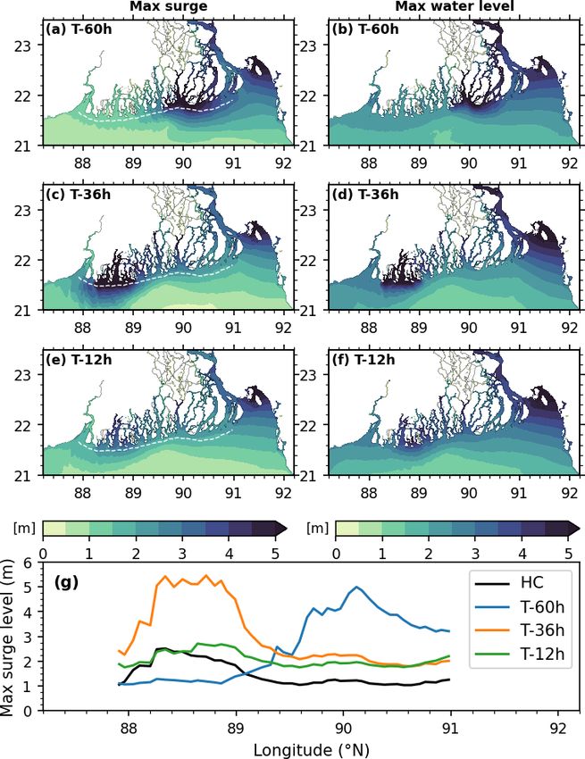
M. J. U. Khan et al.: Chasing the Supercyclone Amphan                                                                                 2527

Figure 2. Conceptual diagram of the involved processes that determine the water level evolution and its interaction with the controls deter-
mining the inland flooding.

Figure 3. Temporal evolution of the successive forecasts of Amphan cyclone wind and pressure. (a) Forecast track colour-coded with the
date (JTWC best track in black). (b) Wind speed forecast with each epoch. (c) Pressure forecast with each epoch. The vertical dashed red
line indicates the time of landfall.

4   Storm surge model and performance                                   as well as barotropic ocean circulation problems for a broad
                                                                        range of spatial scales, from the creek scale to the ocean
                                                                        basins (Ye et al., 2020; Zhang et al., 2020, 2016a). It has
We have developed our tide and storm surge model based
                                                                        already been shown to have an excellent performance in re-
on the community and open-source modelling platform
                                                                        producing shallow-water processes over the Bengal shoreline
SCHISM (Semi-implicit Cross-scale Hydroscience Inte-
                                                                        and elsewhere, including the coastal tide (Krien et al., 2016),
grated System Model) developed by Zhang et al. (2016b)
                                                                        wave set-up (Guérin et al., 2018), and storm surge flooding
– a derivative code of the SELFE (Semi-implicit Eulerian–
                                                                        (Bertin et al., 2014; Krien et al., 2017; Fernández-Montblanc
Lagrangian Finite Element) model, originally developed
                                                                        et al., 2019).
by Zhang and Baptista (2008). This model solves the
shallow-water equations using finite-element and finite-
volume schemes in an unstructured grid that can combine
tri- and quad-elements. The model is applicable in baroclinic

https://doi.org/10.5194/nhess-21-2523-2021                                      Nat. Hazards Earth Syst. Sci., 21, 2523–2541, 2021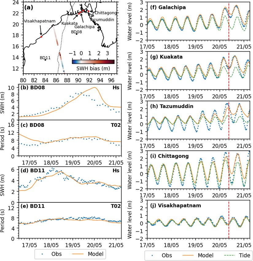
2528                                                              M. J. U. Khan et al.: Chasing the Supercyclone Amphan

4.1    Model implementation                                       slope, the value for the breaking coefficient α, which controls
                                                                  the rate of dissipation, was reduced from 1 to 0.1 to avoid
We have implemented our model on an updated bathymetry            over-dissipation (Pezerat et al., 2020, 2021). The WWMIII
of Krien et al. (2016) with the additional inclusion of 77 000    was also forced along the model’s southern open boundary
digitized sounding points from a set of 34 nautical charts        by time series of directional spectra, computed from a large-
published by the Bangladesh Navy (Khan et al., 2019) (See         scale application of the WaveWatch3 (hereafter WW3) model
Supplement Fig. S1). Our bathymetric dataset is a combina-        (WW3DG, 2019). The WW3 was implemented at the scale
tion of two digitized sounding datasets in the nearshore zone     of the whole Indian Ocean with a spatial resolution of 0.5◦
– one from navigational charts produced by the Bangladesh         and forced by the final analysis (FNL) reanalysis wind data
Navy and another being a bathymetry of the Hooghly es-            at a 3 h time step (National Centers for Environmental Pre-
tuary provided by the IWAI (Inland Waterways Author-              diction, National Weather Service, NOAA, U.S. Department
ity of India). Depending on the sounding points, these ob-        of Commerce, 2015).
servations are 7 to 20 years old. The river bathymetry
is composed of a set of cross-sections obtained from the          4.2   Model forcings
Bangladesh Water Development Board (BWDB), which is
further interpolated at about 300 m resolution using a dedi-      Our model is forced over the whole domain by the astro-
cated 1D river modelling tool and GIS techniques. The south-      nomical tidal potential for the 12 main constituents (2N2,
central part of the delta is composed of a high-resolution        K1, K2, M2, Mu2, N2, Nu2, O1, P1, Q1, S2, T2). At the
(50 m) inland topography (see Supplement Fig. S2). We             southern boundary, we have prescribed a boundary tidal wa-
considered the General Bathymetric Chart of the Oceans            ter level from 26 harmonic constituents (M2, M3, M4, M6,
(GEBCO) 2014 bathymetry to complement in the deeper               M8, Mf, Mm, MN4, MS4, Msf, Mu2, N2, Nu2, O1, P1, Q1,
part of the ocean (https://www.gebco.net/data_and_products/       R2, S1, S2, S4, Ssa, T2, K2, K1, J1, and 2N2) extracted
gridded_bathymetry_data/, last access: 20 June 2020) and the      from the FES2012 global tide model (Carrère et al., 2013). At
Shuttle Radar Topography Mission (SRTM) digital elevation         open upstream-river boundaries of the Ganges and Brahma-
model for the rest of the inland topography as appearing in       putra, a discharge time series from the BWDB is forced
the GEBCO 2014 dataset (https://www2.jpl.nasa.gov/srtm/           for the benchmark tidal simulation, and a climatologic dis-
cbanddataproducts.html, last access: 20 June 2020). Our un-       charge time series is applied for storm surge simulations dur-
structured model mesh was developed based on this blended         ing Amphan. A discharge climatology is applied at Hooghly
bathymetry, covering the northern Bay of Bengal (11 to            (Mukhopadhyay et al., 2006) and Karnaphuli (Chowdhury
24◦ N) with a variable resolution based on the shallow-water      and Al Rahim, 2012). At Meghna and Rupnarayan open river
wave propagation and bottom slope criteria. Our model grid        boundaries, we implemented a radiating Flather boundary
consists of about 600 000 nodes and 1 million elements in         condition. From a year-long tidal simulation, we found that
total. The resulting grid resolution ranges from 250 m in the     the updated version of the bathymetry performs 2–4 times
estuaries and the delta to 15 km in the deeper part of the cen-   better at key locations compared to the global tidal mod-
tral Bay of Bengal. The model domain and mesh are identical       els, which include Finite Element Solution (FES; Carrère
to those presented in Khan et al. (2019) (Fig. 4).                et al., 2013), Goddard Ocean Tide (GOT; Ray, 1999), and
   To account for the effect of short waves on the mean           TOPEX/POSEIDON (TPXO; Egbert and Erofeeva, 2002)
circulation, the Wind Wave Model III (WWMIII), a third-           (see Supplement Table S1).
generation spectral wave model, is coupled at source code            We derived the atmospheric wind and pressure fields for
level with SCHISM in our modelling framework (Roland              SCHISM from a blending of analytical wind field inferred
et al., 2012). In our configuration, the WWMIII solves the        from a parametric wind model (close to the cyclone track)
wave action equation on the native SCHISM grid using a            and background atmospheric field from the Global Forecast
fully implicit scheme. The source terms in our model com-         System (GFS; https://www.ncdc.noaa.gov/data-access/
prise the energy input due to wind (Ardhuin et al., 2010), the    model-data/model-datasets/global-forcast-system-gfs, last
non-linear interaction in deep and shallow water, energy dis-     access: 30 May 2020) reanalysis (farther away) following
sipation in deep and shallow water due to white capping and       Krien et al. (2017, 2018). We used the best-track data of the
wave breaking, and energy dissipation due to bottom friction.     JTWC provided at a 6 h time step as input for the analytical
We run the WWMIII with 12 directional and 12 frequency            wind and pressure field. Here we choose the analytical wind
bins. Every 30 min of SCHISM runtime, water level and cur-        profile of Emanuel and Rotunno (2011) and the analytical
rents are passed to the WWM for calculating the evolution of      pressure field profile of Holland (1980). To be consistent
the wave fields. Calculated wave radiation stress, total sur-     with our forecast described in Sect. 5, the background wind
face stress, and the wave orbital velocity are passed back to     field was generated incrementally from an accumulative
SCHISM before computing the next time step. Wave break-           merging of GFS forecasts for each 6 h forecast window, with
ing is modelled according to Battjes and Janssen (1978). As       a 1 h time step. The analytical and background wind fields
the nearshore region of the Bengal delta has a very mild          were first temporally interpolated every 15 min and overlaid

Nat. Hazards Earth Syst. Sci., 21, 2523–2541, 2021                               https://doi.org/10.5194/nhess-21-2523-2021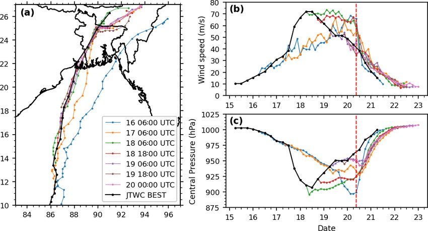
M. J. U. Khan et al.: Chasing the Supercyclone Amphan                                                                           2529

Figure 4. Computational domains and model mesh for SCHISM–WWMIII as well as model boundary conditions. White arrows on the
southern boundary show the forcing with the tidal solution provided by FES2012, and on the northern boundary they show the river dis-
charges. For a hindcast experiment, wave spectra from WW3 are imposed on the southern boundary. The background is taken from Blue
Marble: Next Generation, credited to NASA Earth Observatory.

on the background GFS fields using a distance-varying                on 18 May 2020 at 16:03 GMT. For each altimetric data point
weighting coefficient for the cyclone centre to ensure a             inside our domain, we interpolated the model output using a
smooth transition (Fig. 7b). We took into account the asym-          nearest-neighbour approach, both spatially and temporally.
metry of the cyclonic wind field following Lin and Chavas            This comparison shows that SWH is reasonably reproduced,
(2012). The final resolution after merging the analytical            with RMSE typically within 1 m (within 18 % of the mean
wind field with the interpolated background GFS fields is            value). However, we observed an overestimation of SWH of
0.025◦ . For all storm surge simulations, a spinup time of 2 d       about 2.5 m near the cyclone centre. One of the reasons for
is considered in this study.                                         such a difference is a limitation of analytical wind field mod-
                                                                     els, as discussed by Krien et al. (2017).
4.3   Predictive skills                                                 We present an in-situ-observed time series of SWH and
                                                                     mean wave period during the life cycle of Amphan in Fig. 5
With the above-described model set-up, we ran our model              for BD08 (Fig. 5b–c) and BD11 (Fig. 5d–e) oceanographic
to calculate the water level and sea state evolution during          buoys (the dataset is collected from the Indian National
Amphan. The simulation was done a posteriori once the cy-            Centre for Ocean Information Services (INCOIS) data por-
clone had passed and with JTWC and GFS hindcasts be-                 tal at https://incois.gov.in/portal/datainfo/mb.jsp, last access:
ing already available throughout the cyclone lifetime. Fig-          30 May 2020). The two buoys are located on either side of
ure 5 shows comparisons between observed and modelled                the Amphan track, 250 km to its east and 230 km to its west,
significant wave height (SWH), peak wave period, and wa-             respectively. We can see that at both locations, the model re-
ter level. First, we compare the significant wave height de-         produces the SWH well. The match is particularly good at
rived from the altimetric estimate of Sentinel-3B processed          BD11, consistently within 1 m of the observed evolution. At
by the Wave Thematic Assembly Center from the Coperni-               BD08, SWH is found to be overestimated by about 2 m at
cus Marine Environment Monitoring Service (https://scihub.           its peak, with a 12 h lead shift in time. Such a difference can
copernicus.eu/, last access: 18 June 2020), which overpassed

https://doi.org/10.5194/nhess-21-2523-2021                                  Nat. Hazards Earth Syst. Sci., 21, 2523–2541, 2021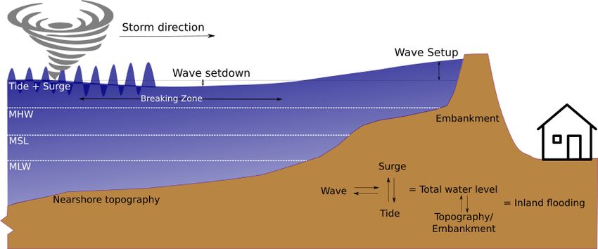
2530                                                                     M. J. U. Khan et al.: Chasing the Supercyclone Amphan

Figure 5. Comparison of simulated (in orange) and observed (in blue) water level, significant wave height (SWH), and mean wave period. (a)
The map shows the along-track bias in SWH compared to the one calculated from Sentinel-3B altimeter overpass at 18 May 2020 16:03 Z.
The bottom panel shows the modelled SWH and mean wave period (orange line) compared to buoy observations (blue dots) at BD08 (b–
c) and BD11 (d–e) provided by INCOIS. Comparison between observed (blue dots) and modelled (orange line) water level at the station
locations – (f) Galachipa, (g) Kuakata, (h) Tazumuddin, (i) Chittagong, and (j) Visakhapatnam. Green dashed lines in (f)–(k) indicate the
modelled tidal water level. Locations of the buoys and the water level gauges are shown in (a). The vertical red lines in water level plots
indicate the time of landfall.

come from positional and timing uncertainties in JTWC best-             of capturing the general features of the sea state, both sig-
track data, from our assumption of a constant translational             nificant wave height (SWH) and period, relatively well. The
velocity in between each 6-hourly JTWC time step, and fi-               overall predictive skills of the model in terms of short waves
nally from the intrinsic uncertainty in the analytical wind             are only slightly below those from hindcast exercises typi-
field itself, as shown in Fig. 3b. Despite multiple sources of          cally conducted over other ocean basins using similar mod-
potential errors and uncertainties, our model appears capable           elling strategies (Bertin et al., 2014; Krien et al., 2018).

Nat. Hazards Earth Syst. Sci., 21, 2523–2541, 2021                                      https://doi.org/10.5194/nhess-21-2523-2021
M. J. U. Khan et al.: Chasing the Supercyclone Amphan                                                                              2531

   The real-time availability of observed water level time se-
ries in this region is relatively scanty. We were able to ac-
cess only a handful of coastal water level records, most of
them located eastward of the landfall location. The right pan-
els of Fig. 5f–j illustrated the comparison of the recorded
water level and modelled storm surge. Among these tide
gauges, Chittagong (Fig. 5i) and Visakhapatnam (Fig. 5j)
time series are retrieved from the UNESCO Intergovern-
mental Oceanographic Commission (IOC) sea level moni-
toring service (http://www.ioc-sealevelmonitoring.org/map.
php, last access: 18 June 2020), and the rest are provided by
the Bangladesh Inland Water Transport Authority (BIWTA;
http://www.biwta.gov.bd/, last access: 18 June 2020). The
datum for water level time series at Chittagong and Visakha-
patnam is changed from in situ datum to MSL by removing
long-term mean. The time series provided by the BIWTA are
already referenced to MSL and thus kept unchanged. We also
plotted the reconstructed tidal water level from the tidal atlas
derived from our model. The overall tidal propagation is well
simulated in Galachipa and Kuakata, while at Tazumuddin
the simulation tidal range is found to be underestimated. The
local bathymetric error and friction parameterization might
be the source of the discrepancy. Tide gauge at Tazumuddin
is situated at the mouth of the Meghna, where bathymetry
is rapidly changing (Khan et al., 2019). However, our model
correctly reproduces the peak of the water level at all loca-
tions. The maximum recorded water level at these stations
is around 2–2.5 m a.m.s.l., with a storm surge (water level –
tide) of the same order of magnitude.
   To spatially assess the storm surge generated by Cyclone
Amphan, we first take a look into the temporal maximum wa-
ter level in Fig. 6a. We can see that the whole coastal region
experienced a high water level ranging from 2–5 m for Am-
phan. To quantify the contribution of the cyclone, we have
looked in the surge component, defined as the difference be-
tween the total modelled water level and a tide-only simu-
lation. Figure 6b illustrates the temporal maximum of surge
over the delta region. The highest surge level is 5 m around
the location of the landfall (21.6◦ N, 88.3◦ E). The maxi-
mum non-linear interaction between tide and surge amounts          Figure 6. Hindcast of (a) maximum water level, (b) maximum
to about 30 cm in the nearshore domain (Fig. 6d).                  surge, wave set-up and set-down, and (d) maximum non-linear
   To quantify the contribution of the wave set-up, we re-         interaction between tide and surge. For (a), for the areas above
calculated the storm surge without the coupling with the           mean sea level, the water level is converted to water level above
wave model. Figure 6c shows the maximum of the difference          the topography for consistency. The inset maps show a close-up
between the two simulated water levels. In general, wave set-      (75 km × 45 km) of the landfall region. The dashed black line shown
                                                                   in (b) is the segment for error analysis of the forecast experiment in
up contributes to the Amphan storm surge by about 20 cm all
                                                                   Sect. 5.
along the Bengal shoreline and locally over 30 cm close to
the cyclone landfall. Nevertheless, the spatial resolution at
the nearshore region employed in this study (250 m) is still
too coarse for capturing the maximum wave set-up that de-          over large estuaries (Bertin et al., 2015; Fortunato et al.,
velops along the shoreline, where a resolution of a few tens       2017).
of metres should be employed (Guérin et al., 2018). Nonethe-          Our findings reaffirm the necessity of a proper coupling
less, this comparison shows that wave set-up not only is de-       between tide, surge, and wave to forecast the water level
veloped along the shoreline exposed to waves but affects the       evolution. For Amphan, the magnitude of tide–surge interac-
whole delta up to far upstream, a process already observed         tion amounts to about 10 % of the maximum total water level

https://doi.org/10.5194/nhess-21-2523-2021                                Nat. Hazards Earth Syst. Sci., 21, 2523–2541, 2021
2532 M. J. U. Khan et al.: Chasing the Supercyclone Amphan
Table 1. Data sources for the model forcings.
Name Data type Time step Resolution Source
JTWC advisory Text Variable n/a https://www.metoc.navy.mil/jtwc/jtwc.html∗
(6–24 h)
HWRF forecast Text 3h n/a https://www.emc.ncep.noaa.gov/gc_wmb/vxt/HWRF/index.php∗
GFS 4D array (via data 1h 0.25◦ https://nomads.ncep.noaa.gov/dods/gfs_0p25_1hr∗
access protocol, DAP)
FNL netCDF 3h 0.25◦ https://rda.ucar.edu/datasets/ds083.3/∗
n/a: not applicable. ∗ Last access: 30 May 2020.
with spatial variation. Similarly, the magnitude of wave set- The NOAA published their HWRF model advisory for each
up is also spatially varying, with a typical amplitude of 10 %– GFS forecast cycle at 3 h time steps. The GFS provides the
15 % of the maximum total water level. This non-negligible, wind and pressure fields in hourly time steps at a 0.25◦ reg-
non-linear dependency shows the importance of a fully cou- ular spatial grid. The GFS model is initialized 6-hourly at
pled hydrodynamics–wave modelling system for a success- 00:00, 06:00, 12:00, and 18:00 UTC, and the data are avail-
ful forecast of the water levels in the hydrodynamic setting able 3 h after the initialized period.
of the Bengal delta. Our modelling framework showed rea- The wind and pressure fields around the centre of the
sonable accuracy in reproducing observed storm surge water storm are derived analytically from a concatenated JTWC
level along the Bengal coastline. The accuracy is in line with and HWRF. We used GFS data as the background wind and
the typical level of performance of similar systems applied pressure on the outer region of the analytical fields.
elsewhere in the world ocean (Bertin et al., 2015; Fernández- We initiated our forecast cycles on 16 March 2020 at
Montblanc et al., 2019; Suh et al., 2015). The hindcast ex- 06:00 UTC, utilizing the first advisory from the JTWC pub-
periment thus shows the viability of our model for a proof of lished at 03:00 UTC merged with the forecast from the
concept of a real-time forecasting exercise. HWRF issued at 18:00 UTC of the preceding day. We took
the background wind and pressure field from the GFS fore-
cast published at 00:00 UTC. In the subsequent forecast cy-
5 Near-real-time storm surge forecasting cles, we updated the previous track file by first replacing the
past time steps with the analysis from the latest JTWC ad-
The current state of maturity of atmospheric real-time cy-
visory, then appending the forecasts from the HWRF again.
clone forecast products allows their application to real-time
For the background wind and pressure fields from the GFS,
surge forecasting, as discussed in Sect. 3. As explained in
we retained the first 6 h of forecasts from the previous cycles
Sect. 2, the storm surge generated from cyclones depends on
and updated the remainder of the time series from the latest
the atmospheric pressure, wind, and background (typically
forecast with new initialization. For each forecast cycle, we
tidal) water level. In this section, a near-real-time storm surge
kept the starting time of our model the same, on 16 May at
forecasting scheme is presented using a publicly available at-
00:00 UTC, and ran it until 1 d after the landfall for a consis-
mospheric forcing dataset.
tent initial condition. This approach is feasible as the storms
5.1 Forecast strategy and forcing products in the Bay of Bengal typically form, grow, and dissipate in
about a week. A graphical representation of our strategy to
During Cyclone Amphan, we performed near-real-time temporally concatenate JTWC, GFS, and HWRF forecasts
storm surge forecasts based on our model. In our forecasts, over a forecast cycle is shown in Fig. 7a. The spatial blend-
we relied on the outputs of global models (GFS and HWRF) ing of the analytical and GFS wind and pressure field is il-
and advisories (JTWC) for the estimates of the atmospheric lustrated in Fig. 7b.
forcing. These advisories and global models are updated ev-
ery 6 h. Similar to the GFS forecast cycle, we updated our 5.2 Real-time computation and results
forecasts at every 00:00, 06:00, 12:00, and 18:00 UTC.
For each forecast, we derived the atmospheric forcing Since our forecast is contingent on the JTWC advisory of
from a blend of JTWC, HWRF, and GFS data (Table 1). The 3 h before, we only had a 3-hour-long window to achieve the
JTWC publishes storm advisories at 03:00, 09:00, 15:00, and pre-processing of the forcing files, to run the model, and to
21:00 UTC. The advisory includes an analysis of the storm complete the necessary post-processing of the model outputs.
intensity and position from a satellite fix 3 h prior, followed The numerical efficiency of our model made it possible to
by a forecast for the following 72 h, with 6 to 12 h time steps. cope with this time constraint of the forecast, using a modest
Nat. Hazards Earth Syst. Sci., 21, 2523–2541, 2021 https://doi.org/10.5194/nhess-21-2523-2021M. J. U. Khan et al.: Chasing the Supercyclone Amphan 2533
Figure 7. (a) Temporal combination scheme of the JTWC, GFS, and HWRF forecasts for each 6-hourly storm surge forecast epoch. (b)
Spatial blending of the analytical and GFS wind and pressure field.
Table 2. Computing environment used during the forecast. the forecast range is notable here. At T − 36 h, the maximum
water level pattern is similar to the hindcast shown in Fig. 6.
Model simulation duration 5.5 d By T − 12 h, the magnitude of the forecast maximum water
Model time step 5 min level corresponds well with the hindcast estimate.
WWM coupling timestamp 30 min To substantiate the gradual increase in the quality of the
Processor clock speed 2.8 GHz forecasts, we compared the maximum surge level predicted
Number of parallel processes 20 at the various forecast ranges (T − 60 h, T − 36 h, T − 12 h)
Wall clock time (pre-processing) 10 min
with the hindcast experiment along a line encompassing the
Wall clock time (model integration) 1 h 45 min
Wall clock time (post-processing) 5 min
nearshore delta (segment displayed in Fig. 6). The results
Disk storage (each simulation) 8 GB show that, in the T − 60 h forecast, the location of maximum
Memory usage 18 GB surge appears offset eastward by as much as 150 km. The
magnitude of the maximum surge is also poorly predicted,
with an overestimation of about 3 m. In the T − 36 h fore-
cast, the location of the maximum surge appears largely cor-
computing resource. The computing environment we used rected, but the magnitude of the peak remains overestimated
is detailed in Table 2, which essentially amounts to a sin- by about 3 m. In the T − 12 h forecast, both the location and
gle desktop computer fitted with a high-end consumer-grade magnitude of the peak surge are in relatively good agreement
processor. with the hindcast. Overall, along this landfalling coastal sec-
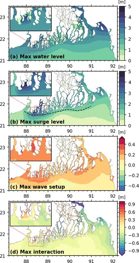
Figure 8 illustrates the evolution of the maximum total wa- tion, the standard error in the maximum surge level amounts
ter level and surge for the corresponding forecasts issued at to 2.06, 1.73, and 0.66 m for the T − 60 h, T − 36 h, and
T −60 h, T −36 h, and T −12 h, where T is the time of land- T − 12 h forecast, respectively.
fall (20 May 2020 at 08:00 to 10:00 UTC). For the forecast
issued at T − 60 h, the cyclone landfall is located near 90◦ E,
associated with the strong surge simulated over the surround-
ing area. As the atmospheric cyclone forecasts gradually con-
verge towards the actual landfall location more than 100 km
westward, so do our storm surge forecasts at T − 36 h and
T − 12 h. The dependency of the timing of the landfall on
https://doi.org/10.5194/nhess-21-2523-2021 Nat. Hazards Earth Syst. Sci., 21, 2523–2541, 20212534 M. J. U. Khan et al.: Chasing the Supercyclone Amphan Figure 8. Maximum surge (a, c, e) and elevation (b, d, f) evolution for forecast initiated at (a–b) T − 60 h (18 May 2020 00:00 Z), (c–d) T − 36 h (19 May 2020 00:00 Z), and (e–f) T − 12 (20 May 2020 00:00 Z) hours before landfall. (g) Comparison of maximum surge level extracted along the section shown by the white line in (a), (c), and (e). Hindcast results (HC) is extracted along the same line shown in Fig. 6b. Nat. Hazards Earth Syst. Sci., 21, 2523–2541, 2021 https://doi.org/10.5194/nhess-21-2523-2021
M. J. U. Khan et al.: Chasing the Supercyclone Amphan                                                                      2535

6     Discussion                                                  of the model to reproduce the water level on the western side
                                                                  of the landfall location due to data unavailability. The proper
6.1    Coupled tide–surge–wave dynamics                           reproduction of the maximum water level by the model gives
                                                                  strong confidence in the formulation as well as in the cou-
The water level dynamics over the Bay of Bengal and par-          pling strategy of our modelling framework.
ticularly around the Bengal delta is complex, and the various
components of water level have different relative contribu-       6.3   Inundation
tions depending on the location. Due to tide–surge interac-
tion, the maximum water level can be lower or higher de-          One of the potential, but challenging, outcomes of storm
pending on the tidal phase in a fully non-linear tide–surge       surge forecasting is the prediction of inundation. Particularly
coupled simulation compared to its linear counterpart. Dur-       in the northern Bay of Bengal, the existing modelling stud-
ing Amphan the tide–surge interaction was mostly negative,        ies do not generally consider the inundation process (Dube
except within about 10 km of the landfall location. The posi-     et al., 2004; Murty et al., 2014). Some modelling systems
tive interaction near the landfall location means that the cou-   take advantage of simplified inundation modelling schemes
pled tide–surge estimate was higher than the linearly added       to tackle this problem (Lewis et al., 2013). In our modelling
tide and surge. In this case, the typical magnitude of tide–      framework, the inland inundation is calculated seamlessly by
surge interaction ranged from −30 to +30 cm. The contri-          SCHISM, solving the same hydrodynamics over the model
bution from the wave-induced set-up along the shoreline in-       domain, thanks to the combination of a cross-scale unstruc-
creases the maximum water level estimation throughout the         tured grid and an efficient wetting–drying algorithm. While
coast by about 10 %–15 % during Amphan.                           the recent improvements in model bathymetry and the de-
                                                                  tailed accounting of dikes and coastal defences improved
6.2    Performance of storm surge forecasting                     the overall modelling of the inundation, the associated er-
                                                                  ror remains large (Krien et al., 2017). As an update to Krien
Aside from the necessary inclusion of relevant physical pro-      et al. (2017), in our model we have incorporated a novel dike
cesses – tide, surge, waves, and their non-linear interactions    height dataset bearing varying dike crest heights for the nu-
– the performance of storm surge forecasting depends on           merous polders scattered around the Bengal delta. The as-
the wind and pressure forcings. The errors in the wind forc-      sessment of the impact of the updated embankment heights
ing and in the atmospheric pressure forcing are typically the     is, however, hard to quantify and validate.
most important ones among the various sources of error in            In the absence of any operational network of inundation
storm surge modelling (Krien et al., 2017). In our forecast       monitoring, to understand and better characterize the inunda-
environment, the source of this error is twofold – the ana-       tion dynamics, we systematically skimmed the Bengal delta
lytical model used to synthesize the fields from the storm        local newspapers on the day of Amphan landfall and on
parameters and the numerical weather model used to fore-          the few subsequent days to achieve an as-comprehensive-
cast the storm wind and pressure fields to derive the storm       as-possible mapping of the inundation extent observed in
parameters themselves. There have been attempts to find a         situ. We digitized the reported flooded locations through
more accurate formulation from recent satellite scatterome-       © Google Earth and categorized the inundation mechanism.
ter missions (Krien et al., 2018). However, not one formula-      We digitized 88 such locations over the Bangladeshi part of
tion works best in all radial distances from the storm centre.    the Bengal delta, as shown in Fig. 9 (Khan, 2020). Over the
Despite the well-known error associated with the paramet-         Indian side of the delta, the news reporting of inland flood-
ric wind field, they are widely used in applications due to       ing from dike breaching was not accurate enough for us to
their computational simplicity and lightweight data require-      be able to geotag the locations. We overlaid the inundated
ments (Lin and Chavas, 2012). The best way to avoid the           locations over the inundation predicted by the model on a
error from the analytical wind field might be not using these     false-colour image derived from the Sentinel-2 satellite using
formulations and relying instead on the full-fledged atmo-        © Google Earth Engine (https://earthengine.google.com, last
spheric forecasts. However, atmospheric models are costly         access: 25 June 2020). Three categories of inundation mech-
in terms of computation. It is particularly true for cyclonic     anism are typically observed – inundation by breaching of
storms where high spatial resolution (typically kilometric) is    the dikes (labelled as “embankment breach”), inundation of
required (Tallapragada et al., 2014).                             unprotected low land by increased water level (“unembanked
   From the validation of water level at a few tide gauge lo-     lowland”), and flooding by overflowing of the dikes (“em-
cations for our hindcast simulation, it appears that the mod-     bankment overflow”). From the reported news, it is clear that
elling framework proposed here could capture the maximum          the major part of the inundation results from the breaching
surge level successfully throughout the coast. Our tide gauge     of dikes. We also note two breaching instances in the south-
sites were limited to the eastern side of the Amphan landfall     eastern corner of our domain, very far from the cyclone land-
location and were operational throughout the life cycle of the    fall. On the other hand, the flooding from merely increased
cyclone. However, it was not possible to confirm the ability      water level in non-diked areas is mostly concentrated along

https://doi.org/10.5194/nhess-21-2523-2021                               Nat. Hazards Earth Syst. Sci., 21, 2523–2541, 2021
2536 M. J. U. Khan et al.: Chasing the Supercyclone Amphan
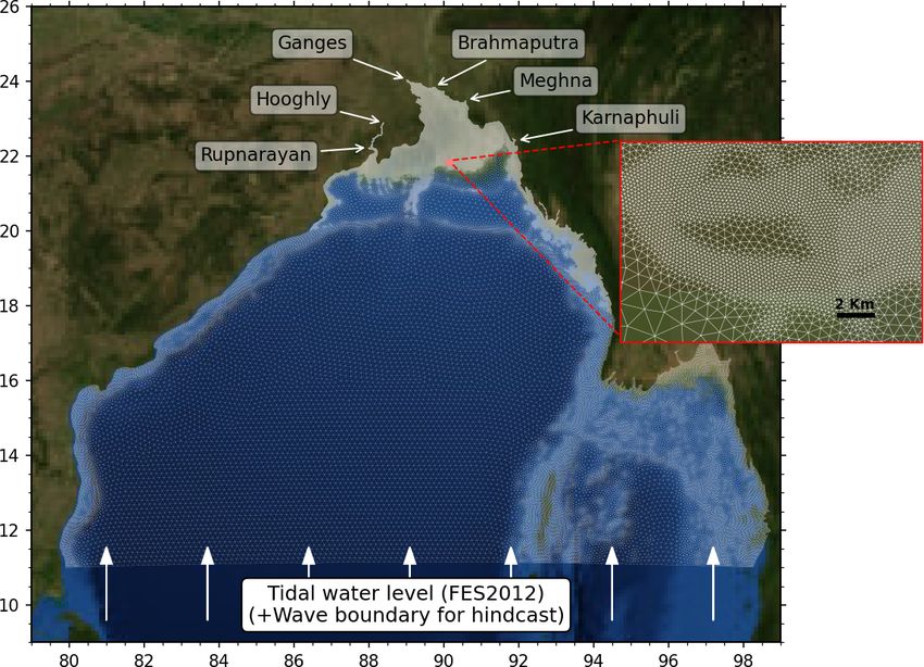
Figure 9. Digitized location of inundation resulting from embankment breaching (red), flooding of low-lying unembanked area (orange),
and embankment overflow (cyan) overlaid on a false-colour image composite derived from B12, B11, and B4 channels of Sentinel-2 during
April 2020. The grey patches are the inundated regions predicted by the model, as shown in the hindcast experiment. The polders are shown
with cyan outlines.
the Meghna estuary. Along the estuary, designed embank- ish waters, which favoured agricultural production by reduc-
ments probably do not exist to protect many populated low- ing the soil salinity (Nowreen et al., 2013). On the other hand,
lying char areas (land or island formed though accretion). these embankments have restricted fresh water and sediment
We could find only one report of the occurrence of overflow- supply, causing significant subsidence inside the embanked
ing of an embankment, in Maheshwaripur of Koyra Upazila areas due to sediment compaction (Auerbach et al., 2015).
(22.45◦ N, 89.30◦ E). Around 22.4–22.6◦ N, 90.1–90.5◦ E, in Over time, the land use inside these polders has also changed
Barishal district, our model predicted an extended inundated from agriculture to aquaculture (namely shrimp and crab
area, which is known to not be polderized. While we could farming). Although the embankments were not built to pro-
find some reports of flooding around that region from our tect from the cyclonic surges, in many instances they func-
newspaper survey, the widespread inundation predicted by tioned as such. The presence of these protective structures
our model in this region probably did not occur in reality due also contributed to a false sense of security among the resi-
to the presence of levees and city protection embankments. dents living inside (Paul and Dutt, 2010). Embankments have
Indeed, this kind of small-scale geographic information, to become part and parcel of survival in this low-lying region.
the best of our knowledge, is not systematically available It has now become essential to monitor the condition and to-
publicly and thus could not be incorporated in our model to- pography of the embankments for efficient management and
pography, despite being of utmost importance for localized maintenance. From a forecasting point of view, embankment
inundation forecasting. The forecast flooded vs. non-flooded breaching is extremely hard to model in the state-of-the-art
areas show a wealth of spatial scales, demonstrating that our hydrodynamic modelling frameworks. However, consistent
unstructured modelling framework has the intrinsic capabil- periodic monitoring of the embankment conditions can im-
ity to model the small-scale hydrodynamic gradients. In our prove the forecast by providing a more objective view of the
modelled forecasts, the contrast between the well-predicted associated inundation hazard.
water level temporal evolution and the comparatively limited
predictive skills of inundated locations points out the neces- 6.4 Prospects in operational forecasting
sity of accurate knowledge and incorporation of reliable to-
pographic and embankment information at the local scale.
Throughout our forecast and hindcast experiments, we have
Our modelling system has the ability and appropriate resolu-
relied on freely available forecast products as the forcing
tion to ingest such topographic information efficiently due to
for our storm surge model. These forecasts data are pub-
its unstructured nature.
licly available within 3 h of their initialization time through
The coastal polder management has long been a boon and
online portals. The primary input to generate the forcing is
a bane (Warner et al., 2018). On one side, the polders have
the forecast storm track distributed as a text file, which is
protected the fertile areas from daily tidal flooding of brack-
very lightweight even for a limited internet connection. We
Nat. Hazards Earth Syst. Sci., 21, 2523–2541, 2021 https://doi.org/10.5194/nhess-21-2523-2021M. J. U. Khan et al.: Chasing the Supercyclone Amphan 2537
have implemented our storm surge model on a freely avail- modelled in our hydrodynamic framework. These two fac-
able open-source framework. The model code is already op- tors call for routine monitoring of embankment topography
erationally used in regional forecasting systems and services and condition.
(Fortunato et al., 2017; Oliveira et al., 2020). Cyclone and storm surge warning has always been a com-
As we have demonstrated, the modelling set-up presented munication and trust issue in the Bay of Bengal (Paul and
here is tractable in an operational, real-time forecasting sce- Dutt, 2010; Roy et al., 2015). It is thus necessary to commu-
nario. Thanks to advanced and efficient numerics, one can nicate well-grounded storm and surge forecasts to the com-
deploy such a system in a consumer-grade computing envi- munity for coordinated and informed decision-making dur-
ronment. The computing set-up we have deliberately used ing a storm surge (Morss et al., 2018). The forecasting sys-
(see Table 2) essentially amounts to a high-end x86-64 per- tem we implemented and assessed in the present case study
sonal desktop computer (e.g. Intel® Core™ i9-10900 or sim- provides the proof of feasibility and opens short-term opera-
ilar). This computing requirement takes only a portion of the tional prospects to fill a gap in the existing disaster manage-
available computing capacity of an institute such as the BMD ment tools in this part of the world.
(15×4 cores at 2.8 GHz) (Roy et al., 2015). Furthermore, the
model is easily deployable in a cloud computing infrastruc-
ture (Oliveira et al., 2020), which could provide additional Code and data availability. The instructions to download and in-
reliability and cost savings for an event-driven operational stall the model used in this study can be accessed freely
forecasting system. at https://github.com/schism-dev/schism (SCHISM development
team, 2020). The sources of the data used in this study are described
in Sects. 4 and 5 of the article. The data should be requested through
the mentioned institutions or downloaded from the provided web-
7 Conclusions sites. The geolocation of inundation mapping from newspapers can
be found at https://doi.org/10.5281/zenodo.4086102 (Khan, 2020).
In this study, we present a retrospective evaluation of storm
surge prediction during Supercyclone Amphan using an effi-
cient, state-of-the-art coupled hydrodynamics–wave numeri- Supplement. The supplement related to this article is available on-
cal model. During Cyclone Amphan, the predicted maximum line at: https://doi.org/10.5194/nhess-21-2523-2021-supplement.
water level ranges from 2 to 5 m along the coastline. Com-
parison with in situ measurements revealed that the water
level could be modelled with high accuracy on the condition Author contributions. MJUK and FD formulated the study. MJUK
that all the relevant mechanisms are considered. Notably, we did the numerical simulations and analysis and wrote the first draft.
demonstrated the necessity of considering a coupled hydro- XB computed the simulation for the WW3 boundary used in the
dynamic tide–surge–wave modelling framework for the head hindcast. All co-authors contributed to this study through multiple
of the Bay of Bengal for effective forecasting. For Amphan, discussions. MP provided help with the WWM formulation. SH dis-
the contribution from tide–surge interaction and wave set-up seminated the forecasts to the local government of Bangladesh and
AKMSI to the scientific community during Cyclone Amphan.
typically amounts to 10 % and 10 %–15 % of the total water
level, respectively.
From our proactive forecast initiative during Cyclone Am-
Competing interests. The authors declare that they have no conflict
phan, we showed that with publicly available storm fore-
of interest.
cast products and easily accessible computing resources, it
is feasible to forecast the evolution of water level through-
out the vast coastline of the Bengal delta in real time. Dur- Disclaimer. Publisher’s note: Copernicus Publications remains
ing Amphan, a sufficiently skilful storm surge forecast was neutral with regard to jurisdictional claims in published maps and
achieved as early as 36–48 h before landfall. The forecast institutional affiliations.
water level with 36 h lead time seemed quite similar to our
hindcast (HC) simulation in terms of maximum water level
as well as the spatial pattern. We communicated the results Acknowledgements. We are thankful to the LIENSs Laboratory
to the Bangladesh local government authority through per- (University of La Rochelle, France) for hosting Md. Jamal Uddin
sonal communications as well as to the scientific community Khan and Laurent Testut during this study.
through social media.
From a secondary post-disaster news survey, we have iden-
tified the limiting factors for location-specific inundation Financial support. This research has been supported by the Centre
forecasts. The main limiting factor is due to limited and National d’Etudes Spatiales (TOSCA BANDINO grant), the em-
outdated topographic information of the existing coastal de- bassy of France in Bangladesh, and the Agence Nationale de la
Recherche (DELTA grant no. ANR-17-CE03-0001).
fences. Also, dike breaching, which was the prevalent pro-
cess of inland inundation during Amphan, is not explicitly
https://doi.org/10.5194/nhess-21-2523-2021 Nat. Hazards Earth Syst. Sci., 21, 2523–2541, 2021You can also read