Constraints on global aerosol number concentration, SO2 and condensation sink in UKESM1 using ATom measurements
←
→
Page content transcription
If your browser does not render page correctly, please read the page content below
Atmos. Chem. Phys., 21, 4979–5014, 2021
https://doi.org/10.5194/acp-21-4979-2021
© Author(s) 2021. This work is distributed under
the Creative Commons Attribution 4.0 License.

Constraints on global aerosol number concentration, SO2 and
condensation sink in UKESM1 using ATom measurements
Ananth Ranjithkumar1 , Hamish Gordon2,1 , Christina Williamson3,4 , Andrew Rollins3 , Kirsty Pringle1 ,
Agnieszka Kupc4,5 , Nathan Luke Abraham6,7 , Charles Brock4 , and Ken Carslaw1
1 School of Earth and Environment, University of Leeds, LS2 9JT, United Kingdom
2 Engineering  Research Accelerator and Centre for Atmospheric Particle Studies, Carnegie Mellon University,
Pittsburgh, PA 15213, USA
3 Cooperative Institute for Research in Environmental Sciences, University of Colorado, Boulder, CO 80309, USA
4 NOAA Chemical Sciences Laboratory, Boulder, CO 80305, USA
5 Faculty of Physics, Aerosol Physics and Environmental Physics, University of Vienna, 1090 Vienna, Austria
6 NCAS-Climate, University of Cambridge, CB2 1EW, UK
7 Department of Chemistry, University of Cambridge, Cambridge, CB2 1EW, UK

Correspondence: Ananth Ranjithkumar (eeara@leeds.ac.uk) and Hamish Gordon (hamish.gordon@cern.ch)

Received: 14 October 2020 – Discussion started: 3 November 2020
Revised: 7 February 2021 – Accepted: 8 February 2021 – Published: 31 March 2021

Abstract. Understanding the vertical distribution of aerosol       boundary layer nucleation scheme. In the boundary layer (be-
helps to reduce the uncertainty in the aerosol life cycle and      low 1 km altitude) and lower troposphere (1–4 km), inclu-
therefore in the estimation of the direct and indirect aerosol     sion of a boundary layer nucleation scheme (Metzger et al.,
forcing. To improve our understanding, we use measure-             2010) is critical to obtaining better agreement with observa-
ments from four deployments of the Atmospheric Tomog-              tions. However, in the mid (4–8 km) and upper troposphere
raphy (ATom) field campaign (ATom1–4) which systemati-             (> 8 km), sub-3 nm particle growth, pH of cloud droplets,
cally sampled aerosol and trace gases over the Pacific and         dimethyl sulfide (DMS) emissions, upper-tropospheric nu-
Atlantic oceans with near pole-to-pole coverage. We evaluate       cleation rate, SO2 gas-scavenging rate and cloud erosion rate
the UK Earth System Model (UKESM1) against ATom ob-                play a more dominant role. We find that perturbations to
servations in terms of joint biases in the vertical profile of     boundary layer nucleation, sub-3 nm growth, cloud droplet
three variables related to new particle formation: total parti-    pH and DMS emissions reduce the boundary layer and up-
cle number concentration (NTotal ), sulfur dioxide (SO2 ) mix-     per tropospheric model bias simultaneously. In a combined
ing ratio and the condensation sink. The NTotal , SO2 and con-     simulation with all four perturbations, the SO2 and conden-
densation sink are interdependent quantities and have a con-       sation sink profiles are in much better agreement with ob-
trolling influence on the vertical profile of each other; there-   servations, but the NTotal profile still shows large deviations,
fore, analysing them simultaneously helps to avoid getting         which suggests a possible structural issue with how nucle-
the right answer for the wrong reasons. The simulated con-         ation or gas/particle transport or aerosol scavenging is han-
densation sink in the baseline model is within a factor of 2       dled in the model. These perturbations are well-motivated in
of observations, but the NTotal and SO2 show much larger bi-       that they improve the physical basis of the model and are
ases mainly in the tropics and high latitudes. We performed a      suitable for implementation in future versions of UKESM.
series of model sensitivity tests to identify atmospheric pro-
cesses that have the strongest influence on overall model per-
formance. The perturbations take the form of global scal-
ing factors or improvements to the representation of atmo-
spheric processes in the model, for example by adding a new

Published by Copernicus Publications on behalf of the European Geosciences Union.
4980                                          A. Ranjithkumar et al.: Constraints on global aerosol number concentration

1   Introduction                                                  CAM3 (Ekman et al., 2012) and ECHAM-HAM (Watson-
                                                                  Parris et al., 2019) with observations.
Aerosols affect the global energy balance directly by scatter-       In this work, we compare in situ aircraft observations con-
ing and absorbing solar radiation and indirectly by their abil-   ducted as part of the NASA Atmospheric Tomography Mis-
ity to act as cloud condensation nuclei (CCN), which changes      sion (ATom) (Wofsy et al., 2018) to a global climate model
the microphysical properties of clouds (Albrecht, 1989;           (UK Earth System Model, UKESM1) to better quantify the
Twomey, 1977). The direct and indirect effects aerosols have      model biases in particle number concentration, SO2 and the
on climate have been identified as the largest source of uncer-   condensation sink. The ATom campaigns provide a represen-
tainty in the assessment of anthropogenic forcing (Bellouin       tative continuous dataset of daytime aerosol, gas and radical
et al., 2020; Carslaw et al., 2013; Myhre et al., 2013). The      concentrations and properties by continuously sampling the
direct radiative forcing by aerosol particles is dependent on     atmosphere vertically and spatially over a vast region of the
the scattering and absorption of solar radiation, which in turn   marine-free troposphere. This single global dataset was ob-
is dependent on aerosol properties like their size, shape and     tained between 2016 and 2018 during four campaigns sam-
refractive index. The indirect radiative forcing is dependent     pling each of the four seasons. During these campaigns, a
on aerosol particles forming or behaving as CCN (or ice nu-       large aerosol and gas instrument payload was deployed on
clei), which is controlled by the hygroscopicity and aerosol      the NASA DC-8 aircraft for systematic sampling of the atmo-
size distribution at cloud base (1–3 km). There are still gaps    sphere spanning altitudes between 0.2 and 12 km, and spa-
in our knowledge of atmospheric processes that control the        tially it encompasses the Pacific and Atlantic oceans with
spatial, temporal and size distribution of aerosols in the at-    near pole-to-pole coverage. These data have been used re-
mosphere. Atmospheric aerosol concentrations depend on            cently (Williamson et al., 2019) to highlight the importance
their sources; primary (emissions) and secondary (new par-        of new particle formation to CCN concentration in the upper
ticle formation and particle growth), their sinks (scavenging,    and free troposphere and to highlight severe deficiencies in
wet and dry deposition) and transport through the atmosphere      the ability of state-of-the-art global chemistry climate mod-
(Merikanto et al., 2009). Thus, the different atmospheric pro-    els to capture new particle formation, particle growth and
cesses that have a controlling influence on the aerosol distri-   aerosol vertical transport accurately.
bution throughout the atmosphere must be better understood.          The ATom data have also been used in previous work to
   Global-scale measurements of aerosol microphysical             address biases in the vertical profile of sea salt and black car-
properties are needed to evaluate general circulation mod-        bon in the Community Earth System Model (CESM) and to
els (GCMs). Satellite measurements have extensive global          better understand the in-cloud removal of aerosols by deep
coverage, but they cannot detect particles smaller than about     convection (Yu et al., 2019). Black carbon lifetime and dif-
100 nm diameter. In situ aircraft measurements give more          ferences in black carbon loading between the Pacific and At-
detailed information about the full size distribution, chem-      lantic basins have also been researched using ATom measure-
ical composition and radiative properties of aerosol parti-       ments (Katich et al., 2018; Lund et al., 2018). Other studies
cles. In past studies (Dunne et al., 2016; Ekman et al., 2012;    used the measurements to address uncertainties associated
Watson-Parris et al., 2019) global models have been com-          with the life cycle of organic aerosol in the remote tropo-
pared against measurement campaigns such as CARIBIC               sphere (Hodzic et al., 2020) and to investigate the mecha-
(Civil Aircraft for Regular Investigation of the Atmosphere       nisms of new particle formation in the tropical upper tropo-
Based on an Instrument) (Heintzenberg et al., 2011), ACE1         sphere (Kupc et al., 2020). The measurements have also shed
(First Aerosol Characterization Experiment) (Clarke et al.,       light on the global distribution of biomass-burning aerosol
1998), PEM Tropics (Pacific Exploratory missions – Trop-          (Schill et al., 2020), brown carbon (Zeng et al., 2020) and
ics) (Clarke et al., 1999), ARCTAS (Arctic Research of the        DMS oxidation chemistry (Veres et al., 2020).
Composition of the Troposphere from Aircraft and Satel-              Although the ATom dataset is extensive and provides im-
lites) (Jacob et al., 2010), PASE (Pacific Atmosphere Sul-        portant information about aerosol number and gas concen-
phur Experiment) (Faloona et al., 2009), INTEX-A (Inter-          trations (Williamson et al., 2019; Wofsy et al., 2018), there
continental chemistry transport experiment – North America)       are some challenges when comparing it to a GCM. A sin-
(Singh et al., 2006) and VOCALS (VAMOS Ocean-Cloud-               gle data point sampled represents a point in the atmosphere
Atmosphere-Land Study) (Wood et al., 2011). Each of these         defined by the latitude, longitude, altitude and time the data
campaigns had goals to help us understand particle size dis-      were collected. The UKESM output is, however, an average
tribution in the upper troposphere, the particle production       over a broad horizontal grid box of ∼ 135 km across, and it is
rate in cloud outflow regions, Arctic atmospheric composi-        usually temporally averaged over a month. In previous stud-
tion, sulfur processing, tropospheric composition over land       ies (Lund et al., 2018; Samset et al., 2018; Schutgens et al.,
and clouds/precipitation in the south-eastern Pacific respec-     2016) it has been shown that sampling errors can be min-
tively. The measurements from these campaigns were used           imised by averaging the observations over time, and model
to identify atmospheric processes that help constrain the par-    errors can be reduced by using 4D model fields with high
ticle size distribution in global climate models like MIT-        temporal resolution. In the first part of this paper, we evalu-

Atmos. Chem. Phys., 21, 4979–5014, 2021                                             https://doi.org/10.5194/acp-21-4979-2021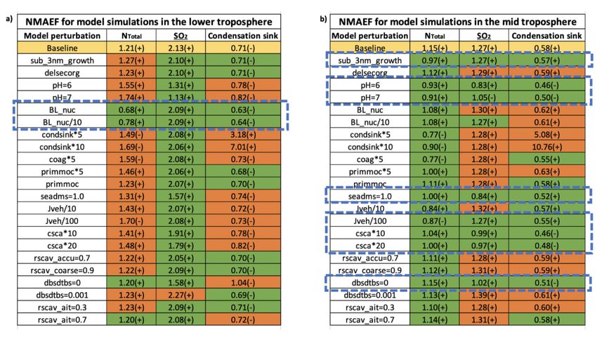
A. Ranjithkumar et al.: Constraints on global aerosol number concentration 4981
ate UKESM at 3-hourly time resolution against observations distribution, composition and optical properties of aerosol
and highlight some of the biases that exist in the model in particles in the remote atmosphere. This can help determine
different regions of Earth. the source of these particles and evaluate the mechanism for
In the second part of this paper, we focus on trying to formation and growth of new particles to form CCN. The
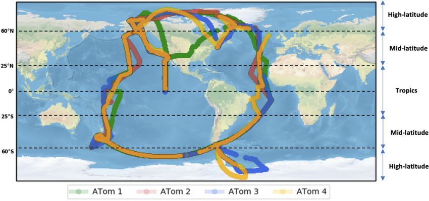
understand and reduce these biases. We focus on processes whole campaign used the NASA DC-8 research aircraft and
related to new particle formation, as this is the dominant was subdivided into four series of flights, ATom1 (August–
source of aerosol number concentration globally (Gordon et September 2016), ATom2 (January–February 2017), ATom3
al., 2017; Yu and Luo, 2009). Some model developments and (September–October 2017) and ATom4 (April–May 2018).
a series of sensitivity simulations are performed to determine The flight path for each of the ATom deployments is shown
the source of the model–measurement bias. As well as re- in Fig. 1. Measurements were made between ∼ 0.18 and
solving a bug in the model, we also address some of the defi- ∼ 12 km altitude, from the Antarctic to the Arctic, over the
ciencies in the nucleation-mode microphysics and the depen- Atlantic and Pacific oceans. All of the data are publicly avail-
dence of coagulation sink on particle diameter. The sensitiv- able (Wofsy et al., 2018).
ity tests comprise model simulations in which we perturb var- We used the SO2 data from ATom4 (the SO2 data from
ious parameters that control different atmospheric processes, ATom1 to 3 were not sensitive at concentrations less than
one at a time. 100 ppt) and the particle number concentration data from
In order to obtain physically motivated reductions in ATom1, ATom2, ATom3 and ATom4. The instruments used
model bias, we evaluate the model simultaneously against to measure the aerosol size distribution from 2.7 nm to
three observed quantities related to new particle formation: 4.8 µm are a nucleation-mode aerosol size spectrometer
total particle number concentration (NTotal ), SO2 mixing (NMASS) (Williamson et al., 2018), an ultra-high-sensitivity
ratio and condensation sink. The condensation sink is a aerosol size spectrometer (UHSAS) and a laser aerosol spec-
measure of how rapidly condensable vapour molecules (in trometer (LAS). The NMASS consists of five continuous
UKESM, sulfuric acid and secondary organic aerosol mate- laminar flow condensation particle counters (CPCs) in par-
rial) and newly formed molecular clusters are removed by allel, with each CPC operated at different settings so as to
the existing aerosol surface area. It is a loss term for new detect different size classes (Brock et al., 2019; Williamson
particles, while SO2 is effectively a production term because et al., 2018). During ATom1, the cut-off sizes (the probabil-
it controls sulfuric acid vapour concentrations. Assessing the ity of the particles at cut-off size of being detected is greater
influence of model processes on only one of these quantities than 50 %) for each of the CPCs were 3.2, 8.3, 14, 27 and
in one-at-a-time sensitivity tests can result in misleading or 59 nm. From ATom2 to ATom4 (more CPCs were present in
incomplete conclusions about model performance, because addition to the CPCs from ATom1), additional cut-off sizes
different atmospheric processes affect NTotal , SO2 and the of 5.2, 6.9, 11, 20 and 38 nm were present. This setup helps
condensation sink to varying degrees and can be indepen- establish the aerosol size distribution for particles smaller
dent of each other. As an example, an atmospheric process than 59 nm. The UHSAS measures particle number concen-
like in-cloud production of sulfate aerosol can increase the trations for particles with diameter between 63 and 1000 nm
condensation sink, which will decrease the gas concentration (Kupc et al., 2018). The LAS efficiently measures particles
of precursors such as sulfuric acid, H2 SO4 , for new particle between 120 nm and 4.8 µm. The POPS instrument was oper-
formation and then in turn decrease NTotal . Perturbing atmo- ated as a backup to detect coarse-mode particles (Gao et al.,
spheric processes can also have a direct effect on the SO2 2016).
mixing ratio and affect H2 SO4 concentration, which controls The SO2 measurements were obtained using the laser-
new particle formation (NPF), and we know from past stud- induced fluorescence instrument (Rollins et al., 2016). SO2
ies (Gordon et al., 2017) that new particle formation is the mixing ratios at high altitudes are quite low (between 1 and
source of about half of the CCN in the atmosphere. Improv- 10 parts per trillion). It is difficult to measure the SO2 mixing
ing the model–observation match to only one of NTotal , SO2 ratio at low pressure with high precision. This instrument is
and the condensation sink can result in a poorer match for capable of retrieving precise measurements of SO2 concen-
the other two quantities. Therefore, it is important to identify tration at pressures as low as 35 hPa, making this instrument
atmospheric processes that reduce NTotal , SO2 and conden- operable up to altitudes of 20 km. The instrument has a de-
sation sink biases simultaneously. tection limit of 2 ppt (at a 10 s measurement interval) and an
overall uncertainty of ± (16 % + 0.9 ppt).
2 The ATom dataset
3 Model description
The main goal of the ATom campaign was to improve our sci-
entific understanding of the chemistry and climate processes The model used in this work is UKESM1 (Mulcahy et al.,
in the remote atmosphere over marine regions. In relation 2020; Sellar et al., 2019) in its atmosphere-only configuration
to aerosols, the campaign helps to quantify the abundance, (with fixed sea surface temperatures and prescribed biogenic
https://doi.org/10.5194/acp-21-4979-2021 Atmos. Chem. Phys., 21, 4979–5014, 2021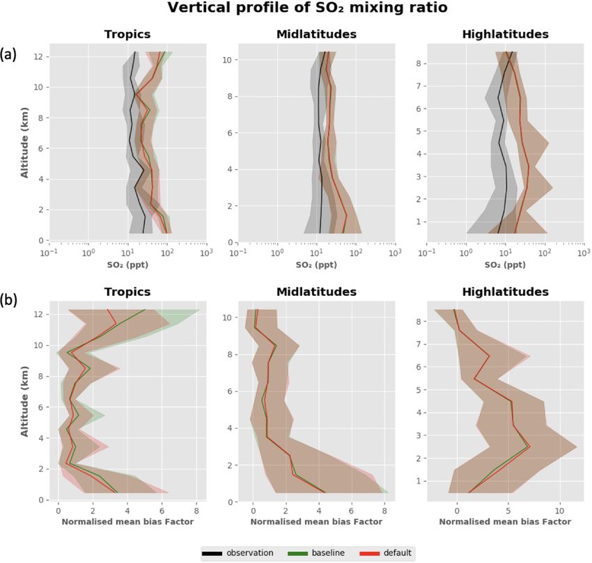
4982                                           A. Ranjithkumar et al.: Constraints on global aerosol number concentration

Figure 1. Flight tracks for NASA DC-8 for the four ATom campaigns: ATom1 (August–September 2016, green), ATom2 (January–
February 2017, red), ATom3 (September–October 2017, blue) and ATom4 (April–May 2018, yellow).

emissions from a fully coupled model simulation). The lat-          al., 2010). However, in this study the UKCA chemistry and
est HadGEM3 global coupled (GC) climate configuration of            aerosol modules are fully coupled (Mulcahy et al., 2020).
the UK Met Office was used to develop UKESM. HadGEM3                   The model can be run in different configurations (Walters
consists of the core physical dynamical processes of the at-        et al., 2017): in this work we use the N96L85 configuration,
mosphere, land, ocean and sea ice systems (Ridley et al.,           which is 1.875◦ × 1.25◦ longitude–latitude, corresponding to
2018; Storkey et al., 2018; Walters et al., 2017). The UK’s         a horizontal resolution of approximately 135 km. The model
contribution to the Coupled Model Intercomparison Project           has 85 vertical levels up to an altitude of 85 km from the
Phase 6 (CMIP 6) (Eyring et al., 2016) is comprised of model        Earth’s surface, with 50 levels between 0 and 18 km and 35
simulations from the HadGEM3 and UKESM1 models.                     levels between 18 and 85 km. To compare the model against
   Atmospheric composition is simulated with the chemistry-         observations, we run the model in a nudged configuration
aerosol component of UKESM, which is the UK Chem-                   over the period during which the ATom campaigns took place
istry and Aerosol model (UKCA) (Morgenstern et al., 2009;           (2016–2018). In this configuration, horizontal winds and po-
O’Connor et al., 2014; Archibald et al., 2020). The anthro-         tential temperature in the model are relaxed towards fields
pogenic, biomass-burning, biogenic and DMS land emis-               from the ERA-Interim reanalysis fields (Dee et al., 2011;
sions used by the model are taken from Hoesly et al. (2018),        Telford et al., 2008). This helps to reproduce the same mete-
van Marle et al. (2017), Sindelarova et al. (2014) and Spiro        orological conditions at the exact time and location the mea-
et al. (1992) respectively. The aerosol scheme within UKCA          surements were performed and to reduce model biases com-
is referred to as the Global Model of Aerosol Processes,            pared to free-running configurations (Kipling et al., 2013;
GLOMAP mode (Mann et al., 2010; Mulcahy et al., 2020).              Zhang et al., 2014). A relaxation time constant of 6 h is cho-
It uses a two-moment pseudo-modal approach and simu-                sen (equal to the temporal resolution of the reanalysis fields),
lates multicomponent global aerosol, which includes sul-            and the nudging is applied between model levels 12 and 80.
fate, black carbon, organic matter and sea spray. Dust is           When comparing the model data to observations, the output
simulated separately using a difference scheme (Woodward,           fields from the model are retrieved at high temporal resolu-
2001). GLOMAP mode includes aerosol microphysical pro-              tion (3-hourly output) at the same times as the observations.
cesses of new particle formation, condensation, coagulation,        This is done to reduce model sampling errors (Schutgens et
wet scavenging, dry deposition and cloud processing. The            al., 2016). The diagnostics fields that we use for our anal-
aerosol particle size distribution is represented using five log-   ysis are total particle number concentration (NTotal ), sulfur
normal modes, nucleation soluble, Aitken soluble, accumu-           dioxide (SO2 ) mixing ratio and condensation sink. These 4D
lation soluble, coarse soluble and Aitken insoluble, with their     diagnostics fields occupy significant disk space, and due to
size ranges shown in Table A1 (Appendix A). UKCA is cou-            storage space constraints, we developed an online interpola-
pled to other modules in UKESM to handle tracer trans-              tor to process the model fields as and when they are output
port by convection, advection and boundary layer mixing.            to give the value of the required diagnostics at the exact time
Originally in GLOMAP mode, sulfate and secondary organic            and location where the measurement was obtained. To reduce
formation was driven by prescribed oxidant fields (Mann et          sampling errors, 5 min averages of the measurements were
                                                                    used in this study. The interpolated diagnostic fields occupy

Atmos. Chem. Phys., 21, 4979–5014, 2021                                               https://doi.org/10.5194/acp-21-4979-2021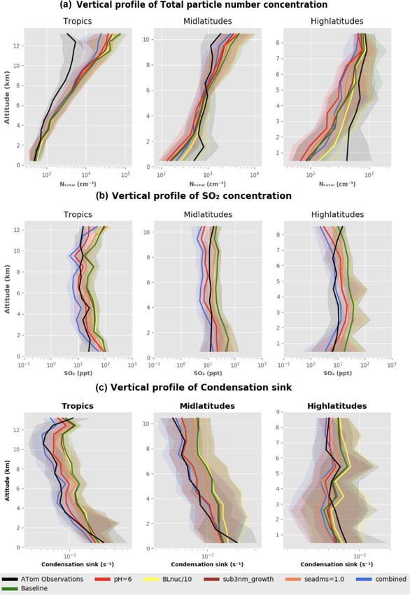
A. Ranjithkumar et al.: Constraints on global aerosol number concentration 4983
less storage space and are retained for our analysis, while the every microphysics timestep, and this was incorrectly imple-
original large model field file is erased. mented: the production of sulfuric acid from SO2 on the mi-
crophysics timestep was missing and the sulfuric acid was
being produced only at the beginning of every chemistry
4 Evaluation of the baseline model timestep. This resulted in an excess H2 SO4 concentration at
the beginning of every chemistry timestep but no production
Figure 2 shows the simulated longitudinal mean fields of to- of H2 SO4 later in the timestep. Nucleation is a very non-
tal particle number concentration (NTotal ), SO2 mixing ra- linear process, and so the high initial H2 SO4 concentration
tio and condensation sink from the atmosphere-only config- resulted in an excessive number of small particles being pro-
uration of UKESM. The particle number concentrations are duced via nucleation. We resolved this bug and used this cor-
much lower at the surface than the free and upper tropo- rected version, which we refer to as the “baseline” version, as
sphere, mainly due to the stronger production rate of new par- the starting point for our sensitivity analysis in Sect. 6. The
ticles via binary homogenous nucleation at higher altitudes. released version of UKESM, which we started with, does
The highest zonal mean NTotal concentration (8 × 10⁴ par- not contain the bug fix and was used in CMIP6 experiments
ticles cm−3 at STP) occurs at an altitude range of 12 to (Eyring et al., 2016). In this study we refer to this version of
16 km. At an altitude of 15 km, most of the particles are the model as the “default” version. Figures 3, 4 and 5 focus
present in the intertropical latitude band (25◦ N–25◦ S). The exclusively on how the baseline version of the model per-
SO2 mixing ratio is maximum (> 1000 ppt) at the surface in forms against observations, and a comparison of how the de-
the Northern Hemisphere because there are significant SO2 fault and baseline versions perform against observations is
sources from land as a consequence of industrial activity. In shown in Appendix Figs. A1, A2 and A3.
the Southern Hemisphere, the SO2 source is mainly from the The SO2 instrument was only flown on the ATom4 cam-
oxidation of dimethyl sulfide emitted from the ocean. The paign, in spring 2018, while the vertical profiles of NTotal and
SO2 mixing ratio at high altitudes is substantial, with a sim- condensation sink are produced using all of the ATom cam-
ulated mixing ratio of ∼ 50 pptv (at 15 km) in the tropics. A paigns, in all four seasons. However, we compare like with
secondary peak in the mixing ratio of SO2 occurs at 30 km like, in that, for example, SO2 observations in spring are
altitude from the oxidation of carbonyl sulfide (we include compared only with SO2 model data at 3-hourly time res-
the stratosphere up to 30 km altitude in Fig. 2 for complete- olution in spring. We perform our analysis using the avail-
ness and the troposphere is the main focus of this study). The able data; however, our analysis could benefit from more SO2
condensation sink is directly related to the number of large data. We can also see that the vertical profiles of NTotal and
particles present in the atmosphere, which provides a surface condensation sink for just ATom4 (Appendix Fig. A4) show
for the condensation of condensable vapours like H2 SO4 . similar biases to Figs. 3 and 5, which have data from all the
Large particles are typically present at a lower altitude; this ATom campaigns aggregated together.
leads to a higher condensation sink close to the surface, Figure 3 compares the simulated and measured vertical
where its maximum value (when longitudinally averaged) is profile of NTotal and the model–measurement normalised
∼ 0.01 s−1 (i.e. the lifetime of condensable vapours before mean bias factor (NMBF) (defined in Eq. 1) (Yu et al., 2006)
condensation is ∼ 100 s). The minimum in the condensation for the baseline simulation. The global data are divided into
sink is around 5 × 10⁻⁵ s−1 , in the upper troposphere. A low three regions: the tropics (25◦ N–25◦ S), mid latitudes (25–
condensation sink at a higher altitude increases the lifetime 60◦ N, 25–60◦ S) and high latitudes (60–90◦ N, 60–90◦ S).
and mixing ratio of condensable vapours like H2 SO4 , which The baseline version of UKESM is shown in green and the
is an important factor in the rapid formation of new particles ATom measurements in black. The magnitude of the model
at these altitudes. bias is quantified by the value 1 + |NMBF|, which is the fac-
To compare the model with ATom data, we use high tem- tor by which the model overestimates or underestimates the
poral resolution 4D model output data along the flight track. observations.
The default version of the model shows substantial biases P
P Mi − 1 = M − 1, if M ≥ O
when compared to observations (Appendix Figs. A1, A2 and OiP O
NMBF = , (1)
A3). On investigating these biases, we discovered a bug in 1 − P Oi = 1 − O , if M < O
Mi M
the subroutine in which the tendency in H2 SO4 concentra-
tion in the chemistry scheme was calculated. The chem- where M indicates the model and O is the observation. A
istry and aerosol processes in the model are handled using positive NMBF indicates that the model prediction is higher
the operator-splitting technique, where the usual timestep for than the measurements and a negative value indicates that the
chemical reactions is 1 h and the algorithm that handles the model is lower than the measurements.
chemistry introduces sub-steps where necessary. Microphys- The default model substantially overpredicts NTotal
ical processes (nucleation, condensation and coagulation) are (Fig. A1) in the upper troposphere (> 8 km), with a factor
treated on a separate 4 min-long sub-timestep within the 1 h of 10–15 overestimate at an altitude of 12 km in the trop-
chemistry timestep. The H2 SO4 concentration is updated on ics. In the lower free troposphere (between 1 and 3 km) and
https://doi.org/10.5194/acp-21-4979-2021 Atmos. Chem. Phys., 21, 4979–5014, 2021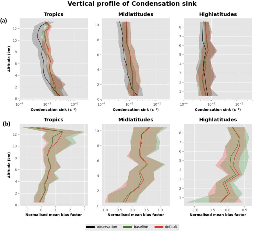
4984                                             A. Ranjithkumar et al.: Constraints on global aerosol number concentration

Figure 2. Global longitudinal mean vertical profile of the simulated (a) total particle number concentration (NTotal ), (b) SO2 mixing ratio
and (c) condensation sink from the default version of our model. In this figure, we show altitudes up to 30 km, and our model top is 85 km,
but our analysis focuses on the troposphere. The black dashed line represents the tropopause height.

boundary layer (< 1 km), the model agrees well (NMBF ∼ 0)               higher concentration of these large particles would result in
with observations in the tropics. However, the model under-             more available surface area for condensable vapours to con-
estimates the observations by a factor of 3 in the mid and              dense. The bias when comparing the model to observations
high latitudes. The baseline (bug-fixed) version of the model           can be explained by uncertainties in primary aerosol/gas
shows biases a factor 5–10 lower in the upper troposphere               emissions or other atmospheric processes. From the verti-
than the default version, for the reasons explained above.              cal profile it appears that the model either transports larger
   Figure 4 shows the vertical profile of the SO2 mixing ratio          aerosol particles to the free troposphere or removes too little
in the model. The baseline model is positively biased by ap-            in precipitation.
proximately a factor 2–6 in the boundary layer regions of the              To explore any longitudinal differences, we also plotted
tropics and mid latitudes. In the tropical upper troposphere,           the observations and model data in the Pacific and Atlantic
the model overpredicts SO2 by up to a factor 2–6, while the             oceans to briefly explore whether the model shows differing
biases in the upper-tropospheric mid and high latitudes are             trends in these regions (Appendix Fig. A5). From the figure
negligible. We speculate that the small differences in biases           we can see that the model shows biases of similar magni-
we see between the baseline and default version (Fig. A2)               tude in the Pacific and Atlantic when compared to observa-
are due to cloud adjustments, which can affect the SO2 con-             tions. The model shows biases of up to 10, 5 and 2 for the
centration and condensation sink. Adjustments arise because             NTotal , SO2 and condensation sink respectively in the Pacific
changes in NTotal can affect cloud drop concentration and liq-          and Atlantic. We also note that we have lumped Northern
uid water path and can therefore change the SO2 lost in aque-           Hemisphere and Southern Hemisphere data for the mid and
ous chemical processing in clouds.                                      high latitudes. The magnitudes of NTotal , SO2 and condensa-
   Figure 5 shows the vertical profile of the condensation sink         tion sink are different in both hemispheres, and we illustrate
in the atmosphere. The condensation sink simulated by the               that in Appendix Fig. A6. The vertical profiles of all three
baseline version of the model shows positive and negative bi-           variables show similar biases in both the northern and south-
ases within a factor of 2 of the observations. Larger particles         ern mid latitudes. In the high latitudes we see more substan-
in the atmosphere contribute to the condensation sink, and a            tial interhemispheric differences. The most notable are that

Atmos. Chem. Phys., 21, 4979–5014, 2021                                                    https://doi.org/10.5194/acp-21-4979-2021
A. Ranjithkumar et al.: Constraints on global aerosol number concentration                                                    4985

(a) NTotal shows a factor of 5 underprediction in the northern      sulfuric acid in the atmosphere, which affects new particle
high-latitude boundary layer, with the southern high-latitude       formation). It should be noted that the H2 SO4 –H2 O nucle-
boundary layer showing good agreement with observations,            ation scheme (Vehkamäki et al., 2002) is an old scheme
and that (b) the model predicts a less than 1 pptv SO2 mixing       and the parameterised nucleation rates are valid only for a
ratio in the southern high latitudes, with observation showing      limited temperature range (230–305 K). A new nucleation
a mixing ratio of ∼ 10 ppt. We explore ways to reduce these         scheme (Määttänen et al., 2018) for the H2 SO4 –H2 O sys-
biases in Sects. 6 and 7.                                           tem extended the validity range to lower temperatures and
   From Figs. 3, 4 and 5, an immediate result of the baseline       a wider range of environmental conditions. Global particle
model evaluation is that the too-high particle number con-          number concentrations for both schemes were compared in
centration in the free and upper troposphere at tropical and        that study (Määttänen et al., 2018), and the vertical profile
mid latitudes is qualitatively consistent with too-high SO2         of particle number concentration was found to be slightly
mixing ratios but inconsistent with the too-high condensa-          higher (by ∼ 100 particles cm−3 ) at lower altitude (between
tion sink. The possible reasons for the biases in NTotal , SO2      300 and 800 hPa), with particle number concentrations in the
and condensation sink are explored later in Sect. 5.                upper troposphere (> 300 hPa) being almost identical. This
                                                                    addresses the uncertainty associated with the Vehkamaki nu-
                                                                    cleation scheme for the H2 SO4 –H2 O system at low temper-
5     Model sensitivity simulations and improvements to             atures in the upper troposphere. However, this perturbation
      model microphysics                                            is not well-motivated by available nucleation parameterisa-
                                                                    tions but is intended only as a candidate for crude tuning to
To investigate the potential causes of the model biases, we         compensate for model biases.
have identified several atmospheric processes that are ex-             Boundary layer nucleation. We incorporated a boundary
pected to influence the vertical profile of the NTotal , SO2 and    layer nucleation (BLN) scheme (Metzger et al., 2010) to ac-
condensation sink. The model simulations that we performed          count for a source of new particles in the boundary layer to
include a combination of direct perturbations to atmospheric        address the model’s boundary layer negative bias (Fig. 5).
processes and changes in model microphysics. The pertur-            Most of our measurements are over the remote ocean, and
bations were applied globally, and we analyse model perfor-         the scheme we use is dependent on oxidation products from
mance at different regions in the troposphere. A more com-          organics which, in our model, originate only from terres-
plete method of sensitivity analysis is to consider the joint ef-   trial vegetation. However, these organic vapours or the nu-
fect of a combination of parameters on model performance,           cleated particles are transported to the remote ocean and
which has been done in the past with perturbed parameter en-        thereby affect the vertical profile. The condensation sink is
semble studies (Lee et al., 2013; Regayre et al., 2018). The        also affected by BLN since the new particles that are formed
one-at-a time sensitivity tests that we carry out here help to      can grow to larger particles by condensation of sulfuric acid
determine which processes have the largest effect on model          and volatile organic compounds onto their surface (Pierce et
biases, and this information can be used in ensemble stud-          al., 2012). We perform one model simulation with boundary
ies in the future. The atmospheric processes which we have          layer nucleation included and then one where the boundary
selected for this study along with the motivation for why we        layer nucleation rate is reduced by a factor of 10. All of the
picked them are described from Sect. 5.1 to 5.5 and also sum-       oxidation products of volatile organic compounds (VOCs)
marised in Table 1. A more detailed analysis of the effect          are treated similarly in the model and have been lumped into
of these model simulations on model biases is described in          a tracer called “Sec_org”. This could lead to biases in the
Sect. 6, and a three-way comparison of NTotal , SO2 and con-        BLN rate and condensational particle growth rate since in re-
densation sink biases is explored in Sect. 7.                       ality the oxidation products of VOCs have different volatili-
                                                                    ties which can nucleate and condense at different rates. Re-
5.1    Nucleation rate and nucleation-mode microphysics             ducing this nucleation rate by a factor of 10 (Regayre et al.,
                                                                    2018; Yoshioka et al., 2019) was found to match better with
Binary homogeneous nucleation. UKESM uses a bi-                     observations.
nary neutral homogeneous H2 SO4 –H2 O nucleation scheme                New particle growth. We improved the handling of the
(Vehkamäki et al., 2002) throughout the atmosphere. The             growth of newly formed clusters in the model because the
upper-tropospheric positive biases in NTotal which we see           initial stage of particle growth up to about 3 nm diameter is
from Fig. 3 could be because of a high nucleation rate. There-      crucial to global CCN concentrations (Gordon et al., 2017;
fore, we perform simulations where we reduce the nucle-             Tröstl et al., 2016) and can affect the vertical profile of par-
ation rate by factors of 10 and 100 to assess its influence         ticle number concentration. Measurement of particle growth
on the large bias in upper-tropospheric particle number con-        rate at diameters smaller than 3 nm is difficult for most at-
centration. These perturbations to the nucleation rate could        mospheric instrumentation. This growth of small particles is
indirectly compensate for the biases in the production rate         determined by competing processes where particles grow by
of H2 SO4 from SO2 (which can affect the concentration of           condensation of vapour onto the particle surface and are lost

https://doi.org/10.5194/acp-21-4979-2021                                             Atmos. Chem. Phys., 21, 4979–5014, 2021
4986                                              A. Ranjithkumar et al.: Constraints on global aerosol number concentration

Figure 3. The first three columns show the vertical profile of the total particle number concentration (at standard temperature and pressure
– STP) as observed (ATom1–4) and in the simulated data from the baseline (bug-fixed) configuration of UKESM in the tropics (25◦ N–
25◦ S), mid latitudes (25–60◦ N and 25–60◦ S) and high latitudes (60–90◦ N and 60–90◦ S). The fourth column shows the NMBF of the
baseline simulation in the tropics, mid latitudes and high latitudes. The bold line represents the median and the shaded region represents the
corresponding interquartile range (25th and 75th percentiles) in a 1 km altitude bin.

Figure 4. The first three columns show the vertical profile of the SO2 (at STP) as observed (ATom4, April–May 2018) and the simulated data
from the baseline (bug-fixed) configuration of UKESM in the tropics (25◦ N–25◦ S), mid latitudes (25–60◦ N and 25–60◦ S) and high latitudes
(60–90◦ N and 60–90◦ S). The fourth column shows the NMBF of the baseline simulation in the tropics, mid latitudes and high latitudes.
The bold line represents the median and the shaded region represents the corresponding interquartile range (25th and 75th percentiles) in a
1 km altitude bin.

Atmos. Chem. Phys., 21, 4979–5014, 2021                                                     https://doi.org/10.5194/acp-21-4979-2021
A. Ranjithkumar et al.: Constraints on global aerosol number concentration                                                             4987

Figure 5. The first three columns show the vertical profile of the condensation sink (at STP) as observed (ATom1–4) and in the simulated data
from the baseline (bug-fixed) configuration of UKESM in the tropics (25◦ N–25◦ S), mid latitudes (25–60◦ N and 25–60◦ S) and high latitudes
(60–90◦ N and 60–90◦ S). The fourth column shows the NMBF of the baseline simulation in the tropics, mid latitudes and high latitudes.
The bold line represents the median and the shaded region represents the corresponding interquartile range (25th and 75th percentiles) in a
1 km altitude bin.

Table 1. Overview of the atmospheric processes that we have chosen for one-at-a-time sensitivity tests and the magnitude of the perturba-
tion/scaling applied.

                             Atmospheric process/parameter           Perturbation to parameter in UKESM
                             pH of cloud droplets                    pH = 6 and 7 (default pH = 5)
                             Boundary layer nucleation               BL_nuc and BL_nuc/10
                             (Metzger et al., 2010)
                             Condensation sink                       condsink × 5 & condsink × 10
                             Primary marine organic emissions        primmoc and primmoc × 5
                             Coagulation sink dependence on          Sub-3 nm growth represented using
                             particle diameter                       Lehtinen et al. (2007)
                             DMS emissions                           Seadms = 1.0 (default = 1.7)
                             Binary H2 SO4 –H2 O nucleation rate     Jveh/10 and Jveh/100
                             SO2 wet-scavenging rate                 csca × 10 and csca × 20
                             Cloud erosion rate                      dbsdtbs = 0 and 10−3
                             Aerosol wet-scavenging efficiency       rscav_ait = 0.3 and 0.7, rscav_accu = 0.7,
                                                                     rscav_coarse = 0.9
                             Coagulation kernel                      coag × 5

https://doi.org/10.5194/acp-21-4979-2021                                                    Atmos. Chem. Phys., 21, 4979–5014, 2021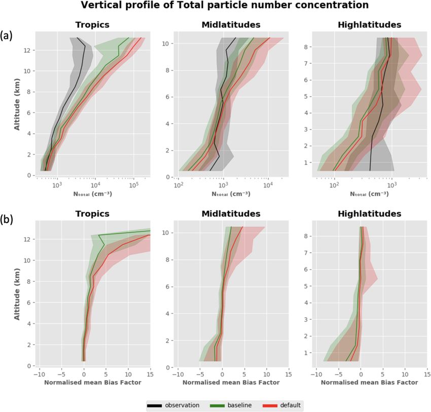
4988                                               A. Ranjithkumar et al.: Constraints on global aerosol number concentration

by coagulation with larger pre-existing particles (Pierce and            densable gases condense onto P aerosol particles in the atmo-
Adams, 2007). Particle growth is simulated explicitly for par-           sphere. It is equal to 2π D j βj dj Nj , where D is the diffu-
ticle sizes larger than 3 nm. However, for the sub-3 nm size             sion coefficient, βj is the transition regime correction factor
range, the growth is represented implicitly by defining an ef-           (Fuchs and Sutugin, 1971), dj is the particle diameter and
fective rate of production of particles at 3 nm (accounting for          Nj is the particle number concentration for the jth aerosol
competing growth and loss processes). This rate is calculated            mode. It is conceivable that the presence of too much sulfu-
using a parametrisation (Kerminen and Kulmala, 2002):                    ric acid in the atmosphere results in the formation of excess
                                                                     new particles, which could explain the bias in NTotal . There-
                   CS(dc ) 2 1       1                                   fore, having a stronger condensation sink could help reduce
J3 nm = Jdc exp            dc    −          ,               (2)
                     GR         3 dc                                     the bias. The model also handles the condensation of H2 SO4
                                                                         and Sec_org differently in that the sulfuric acid concentra-
where J3 nm and Jdc refer to the particle production rate at
                                                                         tion is updated every microphysics timestep (4 min), while
3 nm and the critical size (dc ) respectively, CS (dc ) is the co-
                                                                         the Sec_org concentration is updated only on every chem-
agulation sink for particles of diameter dc onto pre-existing
                                                                         istry timestep (1 h). Since condensation in the atmosphere
aerosol and GR is the growth rate of the particles. The co-
                                                                         can happen on very short timescales, the Sec_org concen-
agulation    sink for a particle of diameter dp is CS(dp ) =
P                                                                        tration may need to be updated at the end of every micro-
   j K(d p , d j ) · Nj , where K(dp dj ) is the coagulation coef-
                                                                         physics timestep as well. We perform model runs after in-
ficient for particles of diameter dp coagulating onto particles
                                                                         corporating this change into the frequency at which Sec_org
of diameter dj . An assumption made to derive Eq. (2) was
                                                                         is updated and also perform simulations where we manually
that the coagulation coefficient for particles was proportional
                                                                         increase the condensation sink by factors of 5 and 10 to see
to the inverse of the square of the particle diameter (∝ dp−2 ).
                                                                         how sensitive the vertical profiles are to this perturbation (the
This is not always a sufficiently good approximation, and the
                                                                         condensation sink can also be indirectly affected by pertur-
power dependency of the coagulation coefficient can vary de-
                                                                         bations to other atmospheric processes). The motivation for
pending on the ambient particle size distribution which varies
                                                                         increasing the condensation sink by large factors was to test
from one location on the planet to another (Kürten et al.,
                                                                         the magnitude of the condensation sink required to reduce
2015). For example, observations at Hyytiala in the Finnish
                                                                         the large biases in NTotal . We only perturb the condensation
boreal forest (Dal Maso et al., 2005) reveal that the power
                                                                         sink directly and not the SO2 or particle number concentra-
law dependency of the coagulation sink with particle diam-
                                                                         tion, because perturbing the condensation sink is technically
eter is not −2: it was in a range between −1.5 and −1.75.
                                                                         more straightforward.
In a previous study (Lehtinen et al., 2007) a new analytical
expression for J3 nm was derived as shown in Eq. (3).
                                                                         5.2   DMS and primary marine organic emissions

                                CS (dc )
J3 nm = Jdc exp −γ · dc ·                  ,                       (3)   There is a significant uncertainty in gas-phase DMS emission
                                  GR
                                                                     from the ocean, because the DMS emission fields are derived
                            s+1                                          from a small set of ocean cruise measurements. Interpola-
where γ = s+1    1       3
                         dc     − 1   and s = log(CS(3 nm)/CS(dc ))
                                                    log(3/dc )      .
                                                                         tion of this small dataset (Kettle and Andreae, 2000; Lana
   We have incorporated this new expression into the model,              et al., 2011) is used to obtain a global DMS emission field
and we show (Sect. 6) that this affects the concentration of             which is used by global models. This results in a large un-
smaller particles in the atmosphere by more correctly ac-                certainty range in the DMS annual budget that lies between
counting for their losses due to coagulation.                            17.6 and 34.4 Tg[S] (Lana et al., 2011). From past studies
   Coagulation sink. The GLOMAP coagulation scheme (Ja-                  (McCoy et al., 2015; O’Dowd et al., 2004) we know that
cobson et al., 1994) includes both inter-modal (collision be-            over marine regions, gas-phase volatile organic compounds
tween particles that belong to different modes) and intra-               emitted from the ocean surface layer are a source of organic-
modal (collision between particles in the same mode) coag-               enriched sea-spray aerosol. We also note that the DMS ox-
ulation. The estimation of the coagulation kernel has uncer-             idation chemistry is also quite uncertain (Hoffmann et al.,
tainties in the effect of Van der Waals forces and charge on             2016; Veres et al., 2020), and this can lead to biases as well.
the particles (Nadykto and Yu, 2003). In this study we are               Our default model version included an emission parametri-
focused only on the overall uncertainty of atmospheric pro-              sation with the DMS field scaled up by a factor of 1.7 to
cesses, so we perturbed the model by scaling up the whole                account for neglecting primary organic aerosol emissions in
coagulation kernel by a factor of 5 to observe its impact on             the model (Mulcahy et al., 2018). This simplified approach
the model–observation comparison.                                        may not be realistic because scaling up DMS emissions will
   Condensation sink. The two condensable species present                result in a larger production of SO2 and H2 SO4 via DMS and
in the model are H2 SO4 (formed from the oxidation of SO2 )              SO2 oxidation. Since our goal is to reduce biases in SO2 and
and Sec_org (formed from the oxidation of monoterpenes).                 particle number, we ran a simulation without the scale fac-
The condensation sink refers to the rate at which these con-             tor of 1.7. More recent versions of the model also include

Atmos. Chem. Phys., 21, 4979–5014, 2021                                                    https://doi.org/10.5194/acp-21-4979-2021
A. Ranjithkumar et al.: Constraints on global aerosol number concentration 4989
an emission parametrisation to estimate the primary marine operator splitting between scavenging and convective trans-
organic aerosol flux, which is significantly correlated with port and simulation of activation above cloud base, which
the chlorophyll concentration (Gantt et al., 2012). Without were subsequently highlighted in other models (Yu et al.,
removing the scale factor of DMS, we tested the sensitivity 2019). As a plume rises through the atmosphere, the change
of aerosol number concentration to this parametrisation by in aerosol number and mass mixing ratios is dependent on
running model simulations with the primary marine organic the precipitation rate, convective updraught mass flux, mass
emissions switched on and also running simulations in which mixing ratio of ice and liquid water, and the scavenging co-
the emissions are scaled up by a factor of 5. efficients (“rscav”) assigned to each mode. The nucleation
mode is not scavenged and is assigned a scavenging coeffi-
5.3 Cloud pH cient of 0; the Aitken, accumulation and coarse modes are
assigned scavenging coefficients of 0.5, 1 and 1 respectively.
Cloud droplet pH is an important parameter in the model be- We assess the sensitivity of the model–observation compar-
cause the aqueous-phase oxidation of SO2 by O3 (to form ison to perturbations in these values. These scavenging co-
sulfate) (Kreidenweis et al., 2003) is very sensitive to the pH efficients used are consistent with convective cloud models
of the cloud droplet. It is assumed in the model that this re- which show that the aerosol in-cloud scavenging is close to
action occurs in all clouds, but the model only tracks the sul- the water-scavenging efficiency (less than 1) (Flossmann and
fate produced in shallow clouds and not in deep convective Wobrock, 2010).
clouds, since most of the sulfate formed would be scavenged We also scale up the convective rain-scavenging rate for all
from the atmosphere by precipitation in convective clouds gases (denoted by the parameter “csca”) by factors of 10 and
but not in non-precipitating or lightly precipitating shallow 20. These have higher uncertainty than aerosol-scavenging
clouds. The rate of this reaction increases by a factor of 105 coefficients because gas uptake into droplets and subsequent
for a pH change from 3 to 6 (Seinfeld and Pandis, 2016). removal depends on gas solubility, temperature, ice forma-
Droplet pH is important because the consumption of SO2 in a tion (and gas retention during freezing), and aqueous-phase
cloud droplet affects the mixing ratio of gas-phase SO2 avail- chemistry (Yin et al., 2002).
able in the atmosphere, thereby reducing the gas-phase con-
centration of H2 SO4 (which can form particles). The cloud 5.5 Cloud erosion rate
pH depends on the thermodynamic and kinetic processes in a
changing cloud droplet distribution, which are not explicitly The cloud erosion rate is an important tuning parameter (rep-
simulated in our model; instead a constant cloud pH of 5 is resented by UKESM parameter “dbsdtbs”) (Yoshioka et al.,
assumed. This assumption could lead to significant errors in 2019) for the prognostic cloud fraction and prognostic con-
regions of the planet where the pH is higher or lower than 5, densate scheme (PC2) used in the model (Wilson et al.,
owing to the regional variability in the amount of acidic and 2008). This parameter determines the rate at which unre-
basic material present in the particles. Since we overestimate solved subgrid motions mix the clear and cloudy air, thereby
SO2 compared to ATom observations, we performed pertur- removing liquid condensate, and it changes the cloud liquid
bations by increasing the pH to 6 and 7 so as to lower the fraction for shallow clouds. Changing this parameter should
SO2 and NTotal bias. This parameter has also been identified have an effect on SO2 lifetime as a result of its uptake into
in previous studies as one of the most important parameters cloud droplets. Its effect on the fraction of cloud in each grid
for global CCN uncertainty (Lee et al., 2013). box will also change the amount of shortwave radiation re-
ceived by the Earth’s surface, which in turn can have feed-
5.4 Scavenging of aerosol particles and gases back effects on aerosol processes. This parameter is usually
tuned so that the outgoing shortwave radiation the model pre-
The removal of aerosol particles and gases in convective dicts matches observations. The default value of “dbsdtbs” in
clouds is an important atmospheric process that can control the model is 1.5 × 10⁻⁴ . We perform two perturbation sim-
the vertical profiles of NTotal , SO2 and condensation sink. ulations with this value set to 0 and another with a value of
Convection in the model is represented using a mass flux 10−3 .
scheme (Gregory and Rowntree, 1990) which is responsible
for the vertical transport of aerosol and gases. Understand-
ing the effect of the removal mechanism for aerosol par- 6 Results
ticles and gases during their vertical transport is crucial in
quantifying their vertical distribution. In the model, aerosol The goal of the model one-at-a-time sensitivity tests is to un-
particles are scavenged using a convective plume-scavenging derstand the causes of biases in the model. Since we are in-
scheme (Kipling et al., 2013), where scavenging coefficients terested in reducing the absolute magnitude of the biases, we
for aerosol particles are assigned for each mode (denoted by use the normalised mean absolute error factor (NMAEF) (Yu
the parameter “rscav”). This convective plume-scavenging et al., 2006) defined in Eq. (4) instead of NMBF to char-
scheme addresses, albeit crudely, biases that resulted from acterise the bias. This new equation allows us to calculate
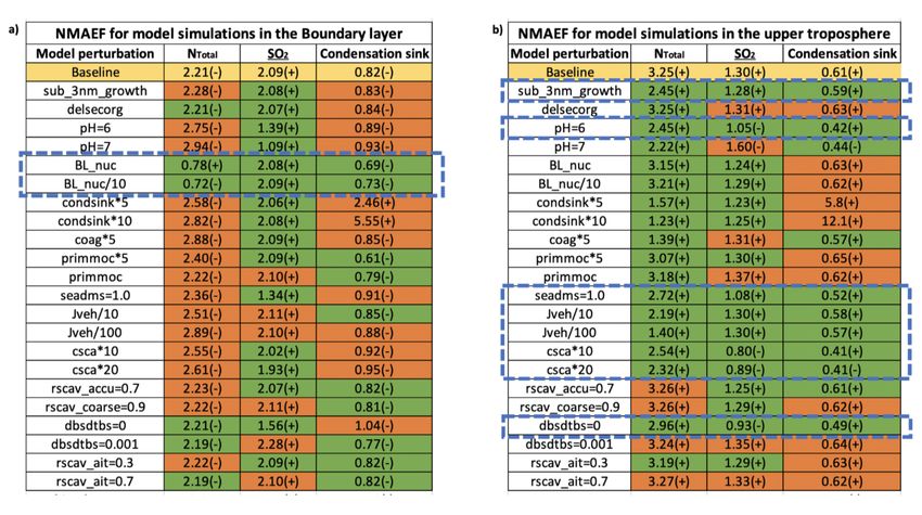
https://doi.org/10.5194/acp-21-4979-2021 Atmos. Chem. Phys., 21, 4979–5014, 20214990 A. Ranjithkumar et al.: Constraints on global aerosol number concentration
the percentage change in model performance as the relative to a simulation with the same nucleation mechanism but with
change in NMAEF of a model experiment with respect to the the nucleation rate reduced by a factor of 10. Including this
baseline version of UKESM as shown in Eq. (5). nucleation mechanism substantially improves model perfor-
P mance by 63 % (NMAEF = 0.78) for “BL_nuc” and 68 %
|M Pi −Oi | , if M ≥ O (NMAEF = 0.72) for “BL_nuc/10”. This is an indication that
NMAEF = P Oi , (4)
|M P i −Oi | , if M < O
the negative model bias in the boundary layer (Fig. 3) could
Mi be explained by a missing boundary layer nucleation mecha-
nism in the model, even though this mechanism depends on
where Mi represents model data, Oi represents observations,
terrestrial emissions of short-lived organic compounds (typi-
M represents the model mean and O represents the mean of cally not found in large concentrations over marine regions).
the observations. A nucleation mechanism other than the Metzger mechanism
Percentage change in model performance (Metzger et al., 2010), which could be a scheme controlled
by chemical species found in the marine boundary layer like
NMAEFsimulation
= 1− × 100 (5) methane sulfonic acid (MSA) (Pham et al., 2005), iodine
NMAEFUKESM_baseline (Cuevas et al., 2018) or ammonia (Dunne et al., 2016), could
The percentage change is zero when the sensitivity test has help reduce model biases even more but is not the focus of
no effect on mean model bias, positive when there is an this work. All the other perturbation simulations either have
reduction in bias, and negative when the bias increases. A no significant effect or decrease NTotal model performance in
model that is in agreement with observations will have an the boundary layer. The perturbation simulations that stand
NMAEF of zero and a percentage improvement of 100 %. out as performing the poorest in the boundary layer are when
Different simulations have varying effects on the vertical pro- we increase the pH (denoted by “pH = 6”, NMAEF = 2.75,
files at different altitudes in the troposphere, and we have and “pH = 7”, NMAEF = 2.94), condensation sink (denoted
therefore split our analysis to study model performance with by “condsink*5”, NMAEF = 2.58, and “condsink*10”,
altitude. The real boundary layer height varies with latitude, NMAEF = 2.89) and scavenging of SO2 (“csca*10”,
but for the purposes of this study we assume it is 1 km ev- NMAEF = 2.55, and “csca*20”, NMAEF = 2.61). These
erywhere. Our results are similar for the boundary layer and perturbations show (Fig. 6a) an approximate decrease of
lower troposphere, suggesting that our analysis is not sen- 25 % in NTotal model performance.
sitive to this assumed boundary layer height. In Sect. 6.1 Secondly, we look at the parameters that significantly im-
we look closely at the model’s performance in the bound- prove the ability of the model to reproduce SO2 mixing
ary layer (which we define here as altitudes below 1 km) and ratios in the boundary layer (Fig. 6b), where the model
lower troposphere (1 km < altitude < 4 km), and in Sect. 6.2 is biased high (NMAEF = 2.09). Figure 6b shows that
we study the mid (4 km < altitude < 8 km) and upper tropo- perturbations to cloud pH, DMS emissions (denoted by
sphere (> 8 km). “seadms = 1.0”), convective rain-scavenging rate (denoted
by “csca*10” and “csca*20”) and the cloud erosion rate (de-
6.1 Boundary layer and lower troposphere noted by “dbsdtbs=0”) all improve model performance. The
DMS emission perturbation, where we removed the artifi-
The performance for the different perturbation simulations cial scaling factor of 1.7 that was used to compensate for
in the boundary layer (altitude < 1 km) can be assessed from the lack of primary marine organics, was also found to im-
Fig. 6. The NMAEF values for the simulations in the bound- prove the model performance by 36 % (NMAEF = 1.34). In-
ary layer are provided in Table 2a. The percentage change in creases in cloud pH from the default value of 5 to 6 or 7 (de-
the bias of NTotal , SO2 mixing ratio, and condensation sink noted in the figure as “pH = 6” and “pH = 7”) improve the
from each of these perturbation simulations is calculated rel- model by 34 % (NMAEF = 1.39) and 48 % (NMAEF = 1.09)
ative to the baseline version of UKESM and is represented respectively. In the atmosphere, a lower cloud pH is typi-
by bar plots. cally associated with polluted environments where particles
Firstly, we look at the model performance with respect to are sulfate-rich, and higher cloud pH is associated with ma-
NTotal in the altitude range 0–1 km, where the model is bi- rine regions where particles are larger and contain carbonates
ased low (Fig. 6a). The baseline version of the model pro- from sea spray (Gurciullo and Pandis, 1997). Therefore, per-
duces boundary layer NTotal values that are negatively bi- turbations to cloud pH by increasing it to 6 or 7 are plausible
ased (NMAEF = 2.21). To reduce the bias in particle num- explanations for the improved model skill since the obser-
ber concentration near the surface, the model perturbation vations are primarily over the remote ocean. Increasing the
simulations (denoted as “BL_nuc” and “BL_nuc/10”) that in- pH increases the rate of the reaction SO2 + O3 → SO2− 4 in
clude a boundary layer nucleation mechanism show the best a cloud droplet, thereby resulting in a larger consumption of
improvement in performance. “BL_nuc” refers to the simu- aqueous SO2 . This drives more SO2 from the gas phase to the
lation that includes the Metzger boundary layer nucleation aqueous phase, thereby reducing the gas-phase SO2 model
mechanism (Metzger et al., 2010), and “BL_nuc/10” refers bias. Increasing the pH can also compensate for the oxida-
Atmos. Chem. Phys., 21, 4979–5014, 2021 https://doi.org/10.5194/acp-21-4979-2021You can also read