PLANT PHENOLOGY EVALUATION OF CRESCENDO LAND SURFACE MODELS - PART 1: START AND END OF THE GROWING SEASON - MPG.PURE
←
→
Page content transcription
If your browser does not render page correctly, please read the page content below
Biogeosciences, 18, 2405–2428, 2021
https://doi.org/10.5194/bg-18-2405-2021
© Author(s) 2021. This work is distributed under
the Creative Commons Attribution 4.0 License.

Plant phenology evaluation of CRESCENDO land surface models –
Part 1: Start and end of the growing season
Daniele Peano1 , Deborah Hemming2 , Stefano Materia1 , Christine Delire3 , Yuanchao Fan4,5 , Emilie Joetzjer3 ,
Hanna Lee4 , Julia E. M. S. Nabel6 , Taejin Park7,8 , Philippe Peylin9 , David Wårlind10 , Andy Wiltshire2,11 , and
Sönke Zaehle12
1 Fondazione   Centro Euro-Mediterraneo sui Cambiamenti Climatici, CSP, Bologna, Italy
2 Met Office Hadley Centre, Exeter, UK
3 Centre National de Recherches Météorologiques, UMR3589, Université de Toulouse/Météo-France/CNRS, Toulouse, France
4 NORCE Norwegian Research Centre AS, Bjerknes Centre for Climate Research, Bergen, Norway
5 Center for the Environment, Harvard University, Cambridge, USA
6 Max Planck Institute for Meteorology, Hamburg, Germany
7 NASA Ames Research Centre, Moffett Field, CA, USA
8 Bay Area Environmental Research Institute, Moffett Field, CA, USA
9 Laboratoire des Sciences du Climat et l’Environnement, Gif-sur-Yvette, France
10 Department of Physical Geography and Ecosystem Science, Faculty of Science, Lund University, Lund, Sweden
11 Global Systems Institute, University of Exeter, Exeter, UK
12 Max Planck Institute for Biogeochemistry, Jena, Germany

Correspondence: Daniele Peano (daniele.peano@cmcc.it)

Received: 26 August 2020 – Discussion started: 4 September 2020
Revised: 15 February 2021 – Accepted: 2 March 2021 – Published: 16 April 2021

Abstract. Plant phenology plays a fundamental role in land–       the timing of the growing season end is accurately simu-
atmosphere interactions, and its variability and variations are   lated in about 25 % of global land grid points versus 16 %
an indicator of climate and environmental changes. For this       in the timing of growing season start. The refinement of phe-
reason, current land surface models include phenology pa-         nology parameterization can lead to better representation of
rameterizations and related biophysical and biogeochemical        vegetation-related energy, water, and carbon cycles in land
processes. In this work, the climatology of the beginning and     surface models, but plant phenology is also affected by plant
end of the growing season, simulated by the land compo-           physiology and soil hydrology processes. Consequently, phe-
nent of seven state-of-the-art European Earth system mod-         nology representation and, in general, vegetation modelling
els participating in the CMIP6, is evaluated globally against     is a complex task, which still needs further improvement,
satellite observations. The assessment is performed using the     evaluation, and multi-model comparison.
vegetation metric leaf area index and a recently developed
approach, named four growing season types. On average, the
land surface models show a 0.6-month delay in the growing
season start, while they are about 0.5 months earlier in the      1   Introduction
growing season end. The difference with observation tends
to be higher in the Southern Hemisphere compared to the           Plant phenology and its variability have a substantial influ-
Northern Hemisphere. High agreement between land surface          ence on the terrestrial ecosystem (e.g. Churkina et al., 2005;
models and observations is exhibited in areas dominated by        Kucharik et al., 2006; Berdanier and Klein, 2011) and land–
broadleaf deciduous trees, while high variability is noted in     atmosphere interactions (e.g. Cleland et al., 2007; Richard-
regions dominated by broadleaf deciduous shrubs. Generally,       son et al., 2013; Keenan et al., 2014). Moreover, recent
                                                                  decades observations show modifications in both spring and

Published by Copernicus Publications on behalf of the European Geosciences Union.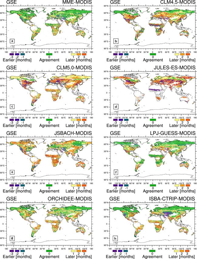
2406                                           D. Peano et al.: Plant phenology evaluation of CRESCENDO LSMs – Part 1

autumn phenology under global warming (e.g. Menzel et al.,         Dubayah, 2017). Besides, some LSMs use satellite-based
2006; Richardson et al., 2013; Park et al., 2016; Zhu et al.,      data assimilation as a tool to constrain the parameters of phe-
2016; Chen et al., 2020; Zhang et al., 2020). For these rea-       nology schemes (e.g. Knorr et al., 2010; Stöckli et al., 2011;
sons, phenology variability is one of the indicators of cli-       MacBean et al., 2015).
mate change (e.g. Schwartz et al., 2006; Soudani et al., 2008;        In this framework, the European CRESCENDO project
Jeong et al., 2011).                                               (https://www.crescendoproject.eu/, last access: 7 June 2020)
   Given the influence of plant phenology on vegetation pro-       fostered the development of a new generation of LSMs to be
ductivity, and since green leaves are the primary interface        used as the land component of the Earth system models (e.g.
for the exchange of energy, mass (e.g. water, nutrient, and        Smith et al., 2014; Olin et al., 2015; Cherchi et al., 2019;
CO2 ), and momentum between the terrestrial surface and the        Mauritsen et al., 2019; Sellar et al., 2020; Seland et al., 2020;
planetary boundary layer (Richardson et al., 2012), land sur-      Yool et al., 2020; Boucher et al., 2020) employed in the Cou-
face models (LSMs) need to accurately simulate plant grow-         pled Model Intercomparison Project Phase 6 (CMIP6, Eyring
ing season cycles. Limitations may result in biases and un-        et al., 2016). In particular, seven novel LSMs, which are part
certainties in representing the vegetation productivity and        of the CRESCENDO effort, are used in this work, namely the
carbon cycle (e.g. Churkina et al., 2005; Kucharik et al.,         Community Land Model (CLM) version 4.5 (Oleson et al.,
2006; Berdanier and Klein, 2011; Richardson et al., 2012;          2013) and version 5.0 (Lawrence et al., 2019), JULES-ES
Friedlingstein et al., 2014; Savoy and Mackay, 2015; Buer-         (Wiltshire et al., 2020a), JSBACH (Mauritsen et al., 2019),
mann et al., 2018). For example, Kucharik et al. (2006)            LPJ-GUESS (Lindeskog et al., 2013; Smith et al., 2014; Olin
show an overestimated April–May net ecosystem produc-              et al., 2015), ORCHIDEE (Krinner et al., 2005), and ISBA-
tion triggered by biases in plant budburst. Berdanier and          CTRIP (Decharme et al., 2019).
Klein (2011) describe a link between above-ground net pri-            Given the relevance of plant phenology and its changing
mary production, growing season length, and soil moisture          variability related to climate, LSMs need routine evaluation
in high-elevation meadows. They show that the potential im-        against observations (e.g. Jolly et al., 2005; Richardson et al.,
pact of changes in active growing season length on biomass         2012; Dalmonech and Zaehle, 2013; Kelley et al., 2013;
production accounts for about 3–4 g m−2 d−1 . The work by          Murray-Tortarolo et al., 2013; Anav et al., 2013; Forkel et al.,
Richardson et al. (2012) is an example of a systematic eval-       2015; Peano et al., 2019). This study aims to evaluate the
uation of LSMs’ phenology representation. They evaluate 14         ability and limits of the novel CRESCENDO LSMs to rep-
models participating in the North American Carbon Program          resent the global climatology of the start and end of growing
Site Synthesis against 10 forested sites, within the AmeriFlux     season timings. The CRESCENDO LSMs cover a wide range
and FLUXNET Canada networks. Their assessment reveals              of phenology schemes and vegetation descriptions. This se-
a typical bias of about 2 weeks in LSM representation of the       lection may therefore help understand the sources of differ-
beginning and end of the growing season. They also show a          ences between LSMs’ representation of phenology and the
low skill in LSMs’ reproduction of the observed inter-annual       regions where plant phenology simulations remain difficult.
phenology variability. These biases lead to an overestima-            Vegetation phenology can be assessed by considering dif-
tion of about 235 gC m−2 yr−1 in the gross ecosystem photo-        ferent plant features and indices, such as leaf colour (e.g. nor-
synthesis of deciduous forest sites. However, uncertainties in     malized difference vegetation index, NDVI, Churkina et al.,
simulated maximum production partially balance this overes-        2005; Keenan et al., 2014), the fraction of absorbed photo-
timation. The work by Buermann et al. (2018) is another ex-        synthetically active radiation (e.g. Kelley et al., 2013; Forkel
ample of a multi-LSM evaluation. They observe widespread           et al., 2015), or canopy density (e.g. LAI, Murray-Tortarolo
lagged plant productivity responses across northern ecosys-        et al., 2013; Peano et al., 2019). Each methodology presents
tems associated with warmer and earlier springs, which is          skills and limitations (e.g Forkel et al., 2015). In this work,
weakly captured by 10 evaluated TRENDYv6 current LSMs.             the novel four growing season types (4GST) methodology
Consequently, current LSMs still present biases in simulating      developed by Peano et al. (2019) is used to evaluate phenol-
timings and the magnitude of the vegetation active season.         ogy. This method proved good skill in capturing the principal
   The latest generation of LSMs have started including a          global phenology cycles (Peano et al., 2019) and integrates
more detailed description of land biophysical and biogeo-          a broader spectrum of growing season modes compared to
chemical processes, and they have become able to explic-           previous techniques (e.g. Murray-Tortarolo et al., 2013). The
itly represent carbon and nitrogen land cycles, as well as         set of growing season modes investigated in 4GST are (1) ev-
plant phenology and related water and energy cycling on            ergreen phenology, (2) single growing season with summer
a global scale (e.g. Oleson et al., 2013; Lawrence et al.,         LAI peak, (3) single growing season with summer dormancy,
2018). In particular, current LSMs link leaf area index (LAI)      and (4) two growing seasons. 4GST uses LAI data to evalu-
and plant phenology to changes in temperature, precipita-          ate phenology. Most ecosystem and climate models introduce
tion, soil moisture, and light availability (e.g. Oleson et al.,   leaf area as a fundamental state parameter describing the in-
2013; Lawrence et al., 2018), as displayed in observations         teractions between the biosphere and the atmosphere. The
(e.g. Caldararu et al., 2012; Zeng et al., 2013; Tang and          most common measure of the area of leaves is the LAI, which

Biogeosciences, 18, 2405–2428, 2021                                                   https://doi.org/10.5194/bg-18-2405-2021
D. Peano et al.: Plant phenology evaluation of CRESCENDO LSMs – Part 1                                                        2407

is generally defined as the one-sided leaf surface area divided             temporal frequency and a 1 km spatial resolution. Note
by the ground area in m2 m−2 (Chen and Black, 1992). In ad-                 that CGLS has a reduced latitudinal coverage compared
dition, LAI is the key variable by which LSMs scale up leaf-                to MODIS and LAI3g since it covers up to 75◦ N versus
level processes to canopy and ecosystem scale exchanges of                  the 90◦ N of the other two products.
carbon, energy, and water. This makes the LAI a reasonable
choice for the evaluation of the LSMs’ phenology (Murray-              The 2000–2011 period is common to the three satellite
Tortarolo et al., 2013; Peano et al., 2019).                        datasets, and it is used in the present analysis. The satel-
   In this paper, we present a brief description of the methods,    lite observations are aggregated into monthly values and re-
LSMs, and satellite data used (Sect. 2). Next, we present the       gridded, by means of a first-order conservative remapping
main results of the satellite data comparison and evaluation        scheme (Jones, 1999), to a regular 0.5◦ × 0.5◦ grid for con-
of LSMs against observations (Sect. 3). Finally, we discuss         sistency with the LSMs’ output. The regridding operation is
the methodology, data, and results (Sect. 4), followed by con-      directly applied to the gap-filled satellite data. Note that re-
cluding remarks (Sect. 5).                                          gridding does not employ any specific treatment for differ-
                                                                    ences in land cover.
                                                                       To perform biome-level analysis, the observed ESA CCI
2     Method, models, and data                                      land cover map (https://www.esa-landcover-cci.org/, last ac-
                                                                    cess: 10 December 2019) has been used to define a stan-
2.1    Satellite observation
                                                                    dard regional vegetation distribution. In particular, Li et al.
To perform a comprehensive global phenology evaluation, a           (2018) aggregated the original 37 ESA CCI land cover
satellite-based observational dataset is required. LAI satel-       classes into 0.5◦ spatial resolution and translated them into
lite observations present uncertainties and limitations related     14 plant functional types (PFTs) based on an adjusted cross-
to the assumptions and algorithms applied in the LAI calcu-         walking table. These data have been used to obtain an ob-
lation (Sect. 4.2, e.g. Fang et al., 2013; Forkel et al., 2015;     served dominant PFT map for the 2000–2011 period. Based
Jiang et al., 2017). For this reason, three different satellite     on Li et al. (2018), all vegetation types are classified into
observational products are considered in this work.                 10 categories: broadleaf evergreen tree (BET), broadleaf
                                                                    deciduous tree (BDT), needle-leaf evergreen tree (NET),
    1. The full time series of LAI3g data is generated by an ar-    needle-leaf deciduous tree (NDT), broadleaf evergreen shrub
       tificial neural network (ANN) algorithm that is trained      (BES), broadleaf deciduous shrub (BDS), needle-leaf ev-
       with the overlapping data of the third-generation Global     ergreen shrub (NES), needle-leaf deciduous shrub (NDS),
       Inventory Modeling and Mapping Studies (GIMMS)               grass-covered areas (Grass), and crop-covered areas (Crop).
       NDVI3g and Terra Moderate Resolution Imaging Spec-
       troradiometer (MODIS) LAI products (see Zhu et al.,          2.2     Land surface models
       2013). It covers the 1982–2011 period with a 15 d tem-
       poral frequency and a 1/12◦ spatial resolution.              Seven European LSMs, which are part of the CRESCENDO
    2. The MODIS (MOD15A2H and MYD15A2H ver-                        project, are evaluated in this study. Further details on each of
       sion 6, https://lpdaac.usgs.gov/, last access: 13 Novem-     these LSMs are provided in the following sections and briefly
       ber 2019; Myneni et al., 2015a, b) LAI algorithm is          summarized in Table 1.
       based on a three-dimensional radiative transfer equation
       that links surface spectral bidirectional reflectance fac-   2.2.1     Community Land Model version 4.5
       tors to vegetation canopy structural parameters (see Yan
       et al., 2016a). It covers the 2000–2017 period with a 4 or   The Community Land Model (CLM) is the terrestrial com-
       8 d temporal frequency and a 500 m spatial resolution.       ponent of the Community Earth System Model version 1.2
                                                                    (CESM1.2, http://www.cesm.ucar.edu/models/cesm1.2/, last
    3. The Copernicus Global Land Service (CGLS, LAI 1 km           access: 1 June 2019). In its version 4.5 (CLM4.5, Oleson
       version 2, https://land.copernicus.eu/global/products/       et al., 2013) and biogeochemical configuration (i.e. BGC
       LAI, last access: 11 March 2020; Maisongrande et al.,        compset, Koven et al., 2013), it is the land component of
       2004; Drusch et al., 2012) LAI dataset is obtained           the CMCC coupled model version 2 (CMCC-CM2, Cher-
       through a neural network applied on top-of-atmosphere        chi et al., 2019). CLM4.5-BGC features 15 PFTs, in which
       input reflectances in red and near-infrared bands de-        crop is represented as a generic C3 crop. The PFTs time
       rived from SPOT and PROBA-V. The instantaneous               evolution follows the area changes described in the Land
       LAI estimates obtained in this way go through a tempo-       Use Harmonization version 2 dataset (LUH2, Hurtt et al.,
       ral smoothing and small gap filling, which discriminate      2020). CLM4.5-BGC resolves explicitly plant phenology
       between evergreen broadleaf forest and no-evergreen          (Oleson et al., 2013; Koven et al., 2013), which is de-
       broadleaf forest pixels (see Verger et al., 2019; Verger     scribed by means of three specific parameterizations: (1) ev-
       et al., 2011). It covers the 1999–2019 period with a 10 d    ergreen plant phenology, (2) seasonal-deciduous plant phe-

https://doi.org/10.5194/bg-18-2405-2021                                                     Biogeosciences, 18, 2405–2428, 2021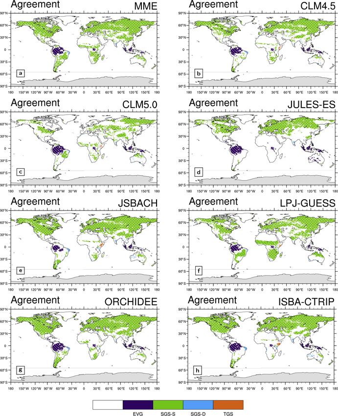
D. Peano et al.: Plant phenology evaluation of CRESCENDO LSMs – Part 1
https://doi.org/10.5194/bg-18-2405-2021
Table 1. (a) Grid spatial resolution used for each land surface model (LSM) and brief summary of their main features. PFT stands for plant functional type and CFT stands for crop
functional type. Part (b) gives further details on the temperature and moisture thresholds for the start (S) and end (E) of the growing season in the phenology schemes.
(a) LSM Original resolution PFT Soil level CFT Phenology scheme Phenology drivers Root zone
CLM 4.5 1.25◦ × 0.9375◦ 15 15 1 C3 evergreen; seasonal deciduous; soil temperature; Zeng (2001)
stress deciduous soil moisture; day length
CLM 5.0 0.5◦ × 0.5◦ 15 20 2 C3 evergreen; seasonal deciduous; soil temperature; moisture Jackson et al. (1996)
stress deciduous day length; precipitation
JULES-ES 1.875◦ × 1.25◦ 13 4 1 C3 , 1 C4 deciduous trees surface temperature Wiltshire et al. (2020a)
JSBACH 1.9◦ × 1.9◦ 12 5 1 C3 , 1 C4 evergreen; summergreen; air temperature; Kleidon (2004)
raingreen; grasses; tropical soil temperature;
crops; extratropical crops soil moisture; NPP
LPJ-GUESS 0.5◦ × 0.5◦ 25 2 3 C3 , 2 C4 evergreen; seasonal deciduous; air temperature; root in top soil layera :
stress deciduous soil moisture Herbaceous PFTs 90 %,
Woody PFTs 60 %
ORCHIDEE 0.5◦ × 0.5◦ 15 11 1 C3 , 1 C4 deciduous; dry and semi-arid; air temperature; exponential profile
grasses and crops soil moisture within the 2 m soil
Krinner et al. (2005)
ISBA-CTRIP 1◦ × 1◦ 16 14 1 C3 , 1 C4 leaf biomass leaf biomass Canadell et al. (1996)
(b) LSM Temperature variable Temperature threshold Moisture variable Moisture threshold Reference
CLM 4.5 third soil layerb temperature 0 ◦ C (S, E) third soil layerb water potential −2 MPa (S, E) Oleson et al. (2013)
CLM 5.0 third soil layerc temperature 0 ◦ C (S, E) third soil layerc water potential −0.6 MPa (S), −2 MPa (E) Lawrence et al. (2018)
JULES-ES mean daily surface temperature depending on PFT and whether none n/a Clark et al. (2011)
S/E: 5 ◦ C, 6.85 ◦ C (S, E)
Biogeosciences, 18, 2405–2428, 2021
JSBACH depending on the phenology: depending on the phenology soil moisture wilting point of Mauritsen et al. (2019)
air, pseudo-soil temperature and whether S/E: 4 ◦ C, 10 ◦ C, in the root zone 0.35 m m−1 (S, E)a Reick et al. (2021)
or critical heat sum (S, E)
LPJ-GUESS mean daily air temperature sum above 5 ◦ C (S) water stress scalar (ω) minimum of ω (ωmin ) (S, E) Smith et al. (2014)
ORCHIDEE mean daily air temperature sum above −5 ◦ C, 0 ◦ C (S) soil moisture in root zone 5 d moisture increase (S) Botta et al. (2000)
weekly temperature depending on PFT: 2, 5, 7, weekly relative soil depending on PFT: Krinner et al. (2005)
10, 12 ◦ C (E) moisture 0.2, 0.3 m3 m−3 (E)
ISBA-CTRIP no phenology model: LAI is deduced from leaf biomass through specific leaf area, which depends on nitrogen content Delire et al. (2020)
a Relative soil moisture content above which growth is possible and below which growth stops and shedding sets in. b About 6 cm depth. c 9 cm depth. n/a – not applicable.
2408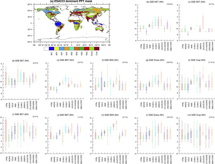
D. Peano et al.: Plant phenology evaluation of CRESCENDO LSMs – Part 1                                                      2409

nology, and (3) stress-deciduous plant phenology (Oleson           2.2.3   JULES-ES
et al., 2013).
   The CLM4.5 representation of phenology is based on soil         JULES-ES is the Earth System configuration of the Joint
temperature, soil moisture, and day length. In particular, the     UK Land Environment Simulator (JULES). JULES-ES is
leaf onset in the seasonal-deciduous plant phenology starts        the terrestrial component of the new UK community ESM,
when the soil temperature of accumulated growing degree            UKESM1 (Sellar et al., 2020). It is based on the core physi-
day (GDD) passes a critical threshold. The leaf litterfall, in-    cal land configuration of JULES (JULES-GL7) as described
stead, starts when the day length exceeds another specific         in Wiltshire et al. (2020a). The simulations described here
threshold (Oleson et al., 2013). In the stress-deciduous plant     used a near-final configuration of JULES-ES prior to the fi-
phenology, soil moisture and soil temperature drive the start      nal tuning performed as part of UKESM1 (Yool et al., 2020).
and end of the growing season. For example, the leaf onset         JULES-ES is run offline forced by global historic meteoro-
is soil-moisture-driven in areas characterized by year-round       logical data as described in Sect. 2.3.
warm conditions. Finally, the evergreen plant phenology is            JULES-ES includes a full carbon and nitrogen cycle with
characterized by a background litterfall, which is a contin-       dynamic vegetation (Wiltshire et al., 2020b), 13 plant func-
uous leaf fall and fine root turnover distributed throughout       tional types with trait-based physiology (Harper et al., 2016),
the year. A PFT-specific leaf longevity parameter drives this      and a representation of crop harvest and land-use change. In
mechanism. Further details can be found in Oleson et al.           JULES-ES, the allometrically defined maximum LAI varies
(2013).                                                            with the carbon status (Clark et al., 2011) and extent of the
                                                                   underlying vegetation. In the case of natural grasses, max-
2.2.2   Community Land Model version 5.0                           imum LAI can vary rapidly sub-seasonally, whereas tree
                                                                   PFTs have a smaller variation. Phenology operates on top of
CLM version 5.0 (CLM5.0) is the terrestrial component of           this variation for deciduous broadleaf and needle-leaf PFTs
the Community Earth System Model version 2 (CESM2,                 based on an accumulated thermal time model. Consequently,
http://www.cesm.ucar.edu/models/cesm2/) and of the Nor-            JULES-ES features one phenology scheme, which relies on
wegian Earth System Model version 2 (NorESM2, Seland               thermal conditions.
et al., 2020).
   CLM5.0 uses the same number of default PFTs, while the          2.2.4   JSBACH
crop module uses two C3 crop configurations: C3 rainfed and
C3 irrigated. The irrigation area is based on crop type and re-    JSBACH3.2 is the land component of MPI-ESM1.2 (Mau-
gion, and the irrigation triggers for crop phenology are newly     ritsen et al., 2019). For the simulations described here, JS-
updated from the CLM4.5.                                           BACH3.2 is run offline at T63 (∼ 1.9◦ ) resolution. Simu-
   CLM5.0 uses the same three specific plant phenology pa-         lations were conducted without natural changes in the land
rameterizations applied in CLM4.5 (Lawrence et al., 2018).         cover; instead, a static map of natural land cover based on
Differently from CLM4.5, CLM5.0 includes also precipita-           Pongratz et al. (2008) was used. Anthropogenic land cover
tion in the stress-deciduous phenology scheme. In particular,      changes were applied using land-use transitions (see Reick
antecedent rain is required to start leaf onset; this is done to   et al., 2013) derived from the LUH2 forcing, whereby range-
reduce the occurrence of anomalous green-up during the dry         lands were treated as natural vegetation (see also Mauritsen
season driven by upwards water movement from wet to dry            et al., 2019). Simulations were conducted according to the
soil layers (Dahlin et al., 2015).                                 common CRESCENDO protocol as described in Sect. 2.3,
   Several major changes have been made in CLM5.0. One of          with the only difference being that land-use change was al-
the physiological changes includes maximum stomatal con-           ready simulated starting at 1700 to avoid a cold start problem
ductance, which now uses the Medlyn conductance model              when applying land-use transitions. JSBACH3.2 contains a
(Medlyn et al., 2011) rather than the previously used Ball–        multilayer hydrology model (Hagemann and Stacke, 2015)
Berry stomatal conductance model. In CLM5.0, the Jack-             and a representation of the terrestrial nitrogen cycle (Goll
son et al. (1996) rooting profiles are used for both water         et al., 2017).
and carbon, where the rooting depths were increased for               JSBACH3.2 is run with its default phenology model,
broadleaf evergreen and broadleaf deciduous tropical tree          called LoGro-P, as evaluated in Böttcher et al. (2016) and
PFTs. These features impact on soil moisture and plant hy-         Dalmonech et al. (2015). This phenology is based on a logis-
drology that control stress-deciduous plant phenology. Other       tic equation for the temporal development of the LAI. Under
modifications that might influence phenology include nu-           ideal environmental conditions, the LAI approaches a max-
trient dynamics, hydrological and snow parameterizations,          imum value representing a prescribed PFT-specific physio-
plant hydraulic functions, revised nitrogen cycling with flex-     logical limit. Growth and leaf shedding rates of the logistic
ible leaf stoichiometry, leaf N optimization for photosynthe-      equation are functions of environmental conditions, chosen
sis, and carbon costs for plant nitrogen uptake (Lawrence          differently according to the phenology type (see e.g. Böttcher
et al., 2019).                                                     et al., 2016). JSBACH3.2 distinguishes the following phe-

https://doi.org/10.5194/bg-18-2405-2021                                                   Biogeosciences, 18, 2405–2428, 2021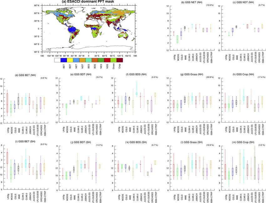
2410                                           D. Peano et al.: Plant phenology evaluation of CRESCENDO LSMs – Part 1

nology types: (1) evergreen, (2) summergreen, (3) raingreen,       (Smith et al., 2014). An explicit phenological cycle is sim-
(4) grasses, and (5) tropical and extratropical crops.             ulated only for leaves and fine roots in seasonal-deciduous
   In general, JSBACH3.2 features a higher amount of phe-          and stress-deciduous PFTs, whereas evergreen PFTs have a
nology schemes (i.e. five) compared to the other LSMs,             prescribed background litterfall for leaves, fine roots, and
which are driven by soil temperature, air temperature, soil        sapwood. Seasonal-deciduous plant phenology is based on a
moisture, and net primary productivity (NPP). In particular,       PFT-dependent accumulated GDD sum threshold for leaf on-
the phase changes in evergreen and summergreen phenolo-            set, with leaf area rising from 0 to the pre-determined annual
gies are determined by temperature thresholds calculated by        maximum leaf area linearly with an additional 200 (100 for
the alternating model of Murray et al. (1989) from heat sums,      herbaceous and needle-leaved tree PFTs) degree days above
chill days, and critical soil temperatures. The raingreen phe-     a threshold of 5 ◦ C. For seasonal-deciduous PFTs, growing
nology has a non-zero growth rate whenever the soil mois-          season length is fixed, with all leaves being shed after the
ture exceeds the wilting point and the NPP is positive. The        equivalent of 210 d with full leaf cover. Stress-deciduous
shedding rate depends on the relative soil water content. The      plant phenology PFTs shed their leaves whenever the water
grass phenology resembles the raingreen phenology but fur-         stress scalar ω drops below a threshold, ωmin , signifying the
ther requires the air temperature and soil moisture to exceed a    onset of a drought period or dry season. New leaves are pro-
critical value for a non-zero growth rate. Because grass roots     duced after a prescribed minimum dormancy period, when ω
are less deep than tree roots, the soil moisture is taken from     again rises above ωmin (Smith et al., 2014). Crop PFT sowing
the upper soil layer for the grass phenology. The crop phenol-     and harvest decisions are modelled based on climate variabil-
ogy is modelled as a function of NPP and distinguishes trop-       ity (Waha et al., 2011; Lindeskog et al., 2013) and climatic
ical and extratropical crops in order to reflect different farm-   thresholds (Bondeau et al., 2007).
ing practices in dependence of the prevailing climatic condi-
tions. The vegetation in the conducted JSBACH3.2 simula-           2.2.6   ORCHIDEE
tions was represented by 12 PFTs, each of which is linked to
one of the phenology types: one forest type with evergreen         The ORCHIDEE model used for the CRESCENDO simula-
phenology, one forest and one shrub type with summergreen          tions is the land component of the IPSL (Institut Pierre Simon
phenology, two forest types and one shrub type with rain-          Laplace) ESM used for the CMIP6 simulations (Boucher
green phenology, C3 and C4 grasses as well as C3 and C4            et al., 2020). The surface heterogeneity is described with 15
pastures with grass phenology, and C3 and C4 crops with ex-        different PFTs that can be mixed in each grid cell. The an-
tratropical and tropical crop phenology, respectively.             nual evolution of the PFT distribution is derived from the
                                                                   LUH2 database as described in more detail in Lurton et al.
2.2.5   LPJ-GUESS                                                  (2019). In each grid cell, the PFTs are grouped into three soil
                                                                   tiles according to their physiological behaviour: high vege-
The Lund–Potsdam–Jena General Ecosystem Simulator ver-             tation (forests) with eight PFTs, low vegetation (grasses and
sion 4.0 (LPJ-GUESS; Lindeskog et al., 2013; Smith et al.,         crops) with six PFTs, and bare soil with one PFT. An inde-
2014; Olin et al., 2015), a process-based second-generation        pendent hydrological budget is calculated for each soil tile
dynamic vegetation and biogeochemistry model, is the ter-          to prevent forests from exhausting all soil moisture. In con-
restrial biosphere component used in the European com-             trast, only one energy budget (and snow budget) is calculated
munity Earth-System Model (EC-Earth-Veg, http://www.               for the whole grid cell. Note that since its first description in
ec-earth.org/, last access: 1 June 2019; Hazeleger and Bin-        Krinner et al. (2005), the model has substantially evolved; we
tanja, 2012; Döscher et al., 2021; Miller et al., 2021). It sim-   describe below only the main features relevant for this study.
ulates vegetation dynamics, land use, and land management             A Phenology module describes leaf onset and leaf senes-
following LUH2 (Hurtt et al., 2020). LPJ-GUESS features            cence for deciduous PFTs based on temperature and soil
25 PFTs, and 10 woody and 2 herbaceous PFTs compete in             moisture. In temperate and boreal regions, leaf onset is driven
the natural stand fractions, whereas two herbaceous species,       by an accumulation of warm temperature in spring, follow-
C3 and C4 photosynthesis pathways, compete in pasture, ur-         ing the concept of GDD. In addition, a minimum period of
ban, and peatland fractions. Crop stands have each five crop       cold temperature, based on a number of chilling days (NCD),
functional types representing the properties of global crop        is used to avoid buds dying with late frosts. Both criteria are
types and correspond to the classes found in LUH2, namely          combined, with PFT-specific GDD and NCD thresholds to be
both annual and perennial C3 and C4 crops, and C3 N fixers,        met before leaves can start growing (see Botta et al., 2000 for
and two herbaceous cover crops (C3 and C4 ) that are grown         more details). For the dry tropics and semi-arid ecosystems,
in between the main agricultural growing seasons.                  a moisture availability criterion is used based on water accu-
   Similar to CLM4.5 and CLM5.0, LPJ-GUESS plant phe-              mulated in the soil. A minimum of 5 consecutive days with
nology is described by means of three specific parameteriza-       soil moisture increase (root zone) should occur after 1 Jan-
tions: (1) evergreen plant phenology, (2) seasonal-deciduous       uary for the Northern Hemisphere and 1 July for the South-
plant phenology, and (3) stress-deciduous plant phenology          ern Hemisphere, with the addition of a filter for small rises

Biogeosciences, 18, 2405–2428, 2021                                                   https://doi.org/10.5194/bg-18-2405-2021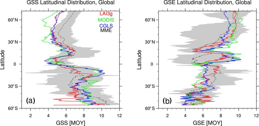
D. Peano et al.: Plant phenology evaluation of CRESCENDO LSMs – Part 1                                                     2411

in soil moisture (see model 4b in Botta et al., 2000). Both        perature, precipitation, wind, surface pressure, shortwave ra-
temperature and moisture criteria are combined for grasses         diation, long-wave radiation, and air humidity.
and crops, and the different parameters of the leaf onset pa-         Each LSM is run on different spatial resolutions (Table 1),
rameterization have been calibrated with satellite data (Botta     but the outputs of these simulations are provided on a regu-
et al., 2000). Leaves are then further separated into four age     lar 0.5◦ × 0.5◦ grid, over which simulations and observations
classes with different photosynthetic efficiency. Leaf fall is     are compared. CLM4.5, JULES-ES, JSBACH, and ISBA-
controlled by different turnover processes. The first one is       CTRIP perform their simulations at a coarser resolution.
a simple ageing process, and a second senescence process           Their output is regridded by applying a first-order conser-
based on climatic conditions (either based on air temperature      vative remapping method (Jones, 1999). The LAI monthly
or soil moisture conditions) is applied.                           mean output from these simulations is used in the present
                                                                   analysis.
2.2.7    ISBA-CTRIP
                                                                   2.4   Growing season analysis
ISBA-CTRIP is the land surface model of CNRM-ESM2-1                The times of the start and end of the growing season (GSS
(http://www.umr-cnrm.fr/spip.php?article1092, last access:         and GSE, respectively) are evaluated using the four grow-
1 June 2019). It is used within the SURFEX version 8               ing season types (4GST) method introduced by Peano et al.
modelling platform representing surface exchanges between          (2019). The 4GST method has been shown to adequately
ocean, lakes, and land. It solves the energy, carbon, and water    capture the main global phenology cycles for evaluation of
budgets at the land surface and was recently thoroughly up-        LSMs.
graded (Decharme et al., 2019). The model distinguishes 16            The 4GST method allows us to evaluate the start and
vegetation types (nine tree, one shrub, three grass, and three     end of the growing season and the global spatial distri-
crop types) alongside desert, rocks, and permanent snow.           bution of four main growing season types: (1) evergreen
Decharme et al. (2019) give a detailed description of the          (EVG), (2) single growing season peaking in summer (SGS-
physical aspects of the model.                                     S), (3) single growing season with summer dormancy (SGS-
   Differently from the other LSMs, leaf phenology results         D), and (4) two growing seasons (TGS). The EVG type is
directly from the daily carbon balance of the leaves. Leaf         identified when relative changes in LAI annual cycle are
turnover time is dependent on potential leaf longevity re-         smaller than 25 % of local LAI mean value. Note that GSS
duced when 10 d assimilation rates start to decrease. Leaf         and GSE timings are not detected in EVG areas. The other
area index is diagnosed from leaf biomass and specific leaf        three types are identified based on LAI slopes and transi-
area index, which varies as a function of leaf nitrogen con-       tion timings as illustrated and summarized in Fig. 1. When
centration and plant functional type. To allow for leaf growth     one single growing season is identified, SGS-S and SGS-D
after dormancy there is an imposed minimum leaf biomass.           are discerned based on the peak month (i.e. in the Northern
Crops have the same phenology as grasses. A detailed de-           Hemisphere (NH), SGS-S is detected when the LAI peak oc-
scription of the terrestrial carbon cycle can be found in Delire   curs between April and September – otherwise, SGS-D is de-
et al. (2020).                                                     tected; the opposite occurs in the Southern Hemisphere (SH):
                                                                   SGS-D is detected when the LAI peak occurs between April
2.3     Experimental setup                                         and September, and SGS-S is identified when LAI peaks in
                                                                   the other months). The timings of the start and end of the
In this study, the S3 CRESCENDO simulations were used,             growing season are identified through a critical threshold
characterized by transient CO2 , climate, and land-use forc-       set to 20 % of the annual LAI cycle (Fig. 1). TGS, instead,
ing. Each model spin-up is obtained by recycling climate           is identified when two growing seasons at least 3 months
mean and variability from the period 1901–1920 with the            long are detected, and GSS and GSE timings are identified
pre-industrial (1860) atmospheric CO2 concentration until          for each cycle. Further details can be found in Peano et al.
carbon pools and fluxes reach a steady state. The 1861–1900        (2019). Note that in this analysis the timings of the TGS GSS
period is simulated using the same climate forcing as the          correspond to the GSS timings of the first growing season cy-
spin-up, but with time-varying atmospheric CO2 and land-           cle, while the GSE timings are the second GSE timings, as
use forcing. Finally, the LSMs are forced over the 1901–2014       described in Peano et al. (2019). The 4GST method is ap-
period with changing CO2 , climate, and land-use forcing.          plied on monthly LAI data in this work, instead of the 15 d
All LSMs are commonly driven by the atmospheric forc-              timescale used in Peano et al. (2019).
ing reanalysis CRUNCEP version 7 (Viovy, 2018), and the
land-use data are taken from the Land Use Harmonization
version 2 dataset (Hurtt et al., 2020). Note that the use of
LUH2 land cover transitions differs across the models (see
model description). CRUNCEPv7 provides for 2 m air tem-

https://doi.org/10.5194/bg-18-2405-2021                                                  Biogeosciences, 18, 2405–2428, 2021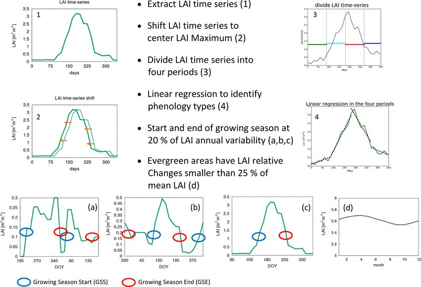
2412                                          D. Peano et al.: Plant phenology evaluation of CRESCENDO LSMs – Part 1

3     Results                                                    of PFTs used by LPJ-GUESS can be the source of this skill
                                                                 (Table 1).
3.1    Satellite data comparison                                    LSMs used in this study are primarily able to capture the
                                                                 observed EVG and SGS-S regions with agreement between
We inspect the main differences between LAI3g, MODIS,            36.0 % and 95.4 % and between 44.3 % and 79.5 %, respec-
and CGLS by plotting the spatial distribution of the four        tively (Table 2). In contrast, the TGS regions are seldom
growing season types, GSS, and GSE (Fig. 2).                     reproduced by LSMs, and the agreement rate with MODIS
   The three products show a high consistency in the distri-     ranges between 0.4 % and 19.1 %, (Table 2). Overall, the
bution of growing season types (agreement of about 80 %,         CRESCENDO multi-model ensemble mean (MME) repro-
Table 2), with the main differences occurring in tropical re-    duces the same MODIS growing-season-type distribution
gions, such as in the Amazon and Congo basins, and in semi-      over about 69.5 % of global land surface area, with a 45.4 %
arid areas, such as central Australia (Fig. 2a, d, g). Com-      to 74.0 % range among models (Fig. 3 and Table 2). It is note-
pared to MODIS, LAI3g differs mainly in EVG regions (Ta-         worthy that the evergreen type is correctly detected in the
ble 2) due to an underestimation of EVG areas in the trop-       broadleaf evergreen tropical areas in both satellite observa-
ics (Fig. S2 in the Supplement). These regions are charac-       tions and LSMs (Fig. 3). On the contrary, the high-latitude
terized by high canopy density, which saturates to high LAI      needle-leaf evergreen regions are partially represented in
in the satellite data (e.g. Myneni et al., 2002), resulting in   LSMs, while satellite data do not catch these areas due to
limited seasonal variability. In addition, the AVHRR sensor      satellite limitations resulting from the impact of cloud and
used to derive LAI3g is less responsive to changes in veg-       snow cover on light availability during the winter season (see
etation compared to MODIS and SPOT/PROBA data (Piao              Sect. 4.2). Besides, the variability of understorey and sec-
et al., 2020). Both LAI3g and CGLS differ from MODIS in          ondary PFTs may influence LAI seasonality representation.
areas featured by the TGS type (Table 2). The Horn of Africa        This initial evaluation highlights that LSMs have difficul-
is the only region where all three satellite products place a    ties in accurately representing SH phenology. The correct
TGS type (Fig. 2).                                               location of the less common types, i.e. single growing sea-
   Larger differences among satellite products are found in      son with summer dormancy (SGS-D) and TGS, is as well
the assessment of GSS and GSE (Fig. 2), especially in            hardly captured by the LSMs. Similar results are obtained
the NH, where LAI3g and CGLS clearly anticipate GSS              when CGLS and LAI3g satellite observations are used as ref-
(Fig. 2e, h) with respect to MODIS. The three satellite prod-    erences (Figs. S2 and S3 and Tables S1 and S2 in the Sup-
ucts present a consistency similar to the one reached by         plement).
the growing-season-type distribution (about 75 %) when a
1-month tolerance is considered (Table 3), since time reso-
lution of the products has been homogenized to 1 month (see      3.3   Variability of growing season start and end
Sect. 2.4).
   Keeping these differences in mind, the MODIS data are         4GST is then applied to evaluate the ability of LSMs to rep-
used as a graphical reference in Figs. 3, 4, and 5. These fig-   resent the GSS and GSE timing in vegetated areas not classi-
ures keep track of the agreement among satellite data despite    fied as EVG type (white regions in Figs. 4 and 5 correspond
the choice of MODIS as reference. Figures using CGLS and         to not-vegetated and EVG-type domains).
LAI3g as a graphical reference are presented in the Supple-         On average at the global scale, LSMs approximately ex-
ment.                                                            hibit a disagreement of 0.6 months and 0.5 months in GSS
                                                                 and GSE, respectively, with LSMs simulating a later GSS
3.2    Growing-season-type distribution                          and an earlier GSE, practically shortening the growing sea-
                                                                 son by 1 month (Table 4). This bias is not evenly distributed
The 4GST allows estimating the ability of each LSM in cap-       around the globe. LSMs reproduce the correct growing sea-
turing the observed spatial distribution of the four growing     son length in about 17 % of the global land grid cell, but
season types (Fig. 3). In general, all the LSMs capture the      sometimes the growing season is affected by a shift in sea-
single growing season that peaks in summer (SGS-S type)          sonality, as in the case of JULES-ES (Table 3). Differently
reasonably well, especially in the NH mid- and high-latitude     from the other LSMs, the LAI cycle in JULES-ES starts from
regions. The majority of LSMs are also able to correctly rep-    a climatological condition (Wiltshire et al., 2020a), which
resent the two growing seasons (TGS) in the Horn of Africa       can lead to the detected shift.
region (Fig. 3). Most LSMs are unable to reproduce the ob-          Generally, the GSE timings simulated by the LSMs show
served growing-season-type distribution in the SH, except for    a better agreement with MODIS (about 25 % agreement in
the evergreen (EVG) tropical areas. A partial exception is       vegetated grid cell, ranging from 4.9 % to 26.4 %, Table 3)
LPJ-GUESS, which shows large SGS-S-type areas in South           compared to GSS timings (15.8 % agreement in vegetated
America, Southern Africa, and northern Australia, in agree-      land grid cell, ranging from 2.7 % to 19.1 %, Table 3). Con-
ment with the satellite products (Fig. 3f). The high number      sidering a 1-month tolerance to account for the downgraded

Biogeosciences, 18, 2405–2428, 2021                                                https://doi.org/10.5194/bg-18-2405-2021
D. Peano et al.: Plant phenology evaluation of CRESCENDO LSMs – Part 1 2413 Figure 1. Scheme of the four growing season types method used in evaluating the start and end of the growing season. Figure 2. Global climatological (averaged over 2000–2011) distribution of (a) the four main growing season modes, (b) growing season start (GSS) timings, and (c) growing season end (GSE) timings for MODIS version 6. The other panels show the comparison between MODIS and LAI3g (second row) and CGLS (third row). In particular, panels (d) and (g) show the areas characterized by the same phenology types (d) between MODIS and LAI3g and (g) between MODIS and CGLS; panels (e) and (h) exhibit the difference in GSS timings; and panels (f) and (i) display the differences in GSE timings. In panels (d) and (g) white areas represent non-vegetated areas and regions of disagreement (d) between MODIS and LAI3g and (g) between MODIS and CGLS. White areas in panel (b), (c), (e), (f), (h), and (i) show evergreen and non-vegetated areas. https://doi.org/10.5194/bg-18-2405-2021 Biogeosciences, 18, 2405–2428, 2021
2414 D. Peano et al.: Plant phenology evaluation of CRESCENDO LSMs – Part 1
Table 2. The fraction of land grid cell in agreement with MODIS for each satellite product and each land surface model in the four growing
season types. Values are reported in percentages and refer to the coloured regions in Fig. 2d and g and Fig. 3.
LAI3g CGLS CLM 4.5 CLM 5.0 JULES-ES JSBACH LPJ-GUESS ORCHIDEE ISBA-CTRIP MME
EVG 10.8 78.3 58.1 72.9 95.4 36.0 55.2 72.3 75.3 51.0
SGS-S 84.4 89.9 64.3 44.3 47.9 71.5 73.8 79.5 74.1 77.2
SGS-D 68.3 80.9 47.6 36.3 7.1 50.6 33.2 33.1 58.8 23.8
TGS 37.2 35.9 19.1 16.9 0.4 13.9 15.4 7.9 12.9 0.7
Total 75.4 86.4 61.2 45.4 48.3 65.2 68.1 74.0 71.1 69.5
Table 3. The fraction of land grid cell in agreement with MODIS for LAI3g, CGLS, each land surface model, and multi-model ensemble
mean (MME) in the growing season start (GSS) and growing season end (GSE) timings. Values are reported in percentages for global,
Northern Hemisphere (NH), and Southern Hemisphere (SH). Green shaded areas in Figs. 4 and 5. The last row reports the fraction of land
grid cell in agreement with MODIS for each land surface model in growing season length. The values in brackets give the percentage of
global, NH, and SH with a maximum difference of 1 month.
LAI3g CGLS CLM 4.5 CLM 5.0 JULES-ES JSBACH LPJ-GUESS ORCHIDEE ISBA-CTRIP MME
GSS 37.9 43.7 14.6 6.5 2.7 16.7 17.3 19.1 16.0 15.8
(74.0) (74.2) (36.1) (21.6) (15.0) (41.3) (45.1) (44.2) (43.1) (31.3)
GSE 45.1 34.0 23.5 6.5 4.9 12.6 20.6 26.4 19.9 25.1
(80.1) (70.5) (44.8) (30.0) (14.7) (38.5) (60.5) (63.8) (62.5) (44.6)
GSS NH 39.2 39.7 15.1 5.7 3.2 17.1 17.6 18.9 16.5 16.3
(76.4) (72.6) (37.8) (20.6) (17.7) (43.4) (44.5) (43.9) (44.5) (32.9)
GSE NH 47.3 29.6 25.4 6.5 6.0 14.4 19.9 29.9 21.7 27.4
(83.6) (68.1) (46.9) (31.2) (17.7) (43.5) (61.0) (69.2) (68.1) (47.5)
GSS SH 32.6 60.7 12.6 10.0 0.7 14.8 16.0 19.8 14.1 13.3
(63.8) (81.0) (28.8) (25.9) (3.4) (32.4) (47.7) (45.6) (36.8) (24.8)
GSE SH 35.9 52.7 15.0 6.6 0.2 5.1 23.4 11.6 12.0 15.5
(64.8) (80.9) (35.7) (24.9) (1.8) (17.5) (58.2) (40.4) (38.7) (32.1)
Length 26.7 28.9 7.9 10.3 9.5 17.4 9.2 12.7 13.7 16.7
(60.6) (54.2) (28.4) (33.7) (27.0) (45.3) (31.9) (39.1) (35.2) (35.2)
time resolution, the agreement between LSMs and MODIS schemes driven by temperature and soil moisture versus one
increases to ∼ 45 % and ∼ 31 %, respectively (Table 3). parameterization only based on the temperature in JULES-
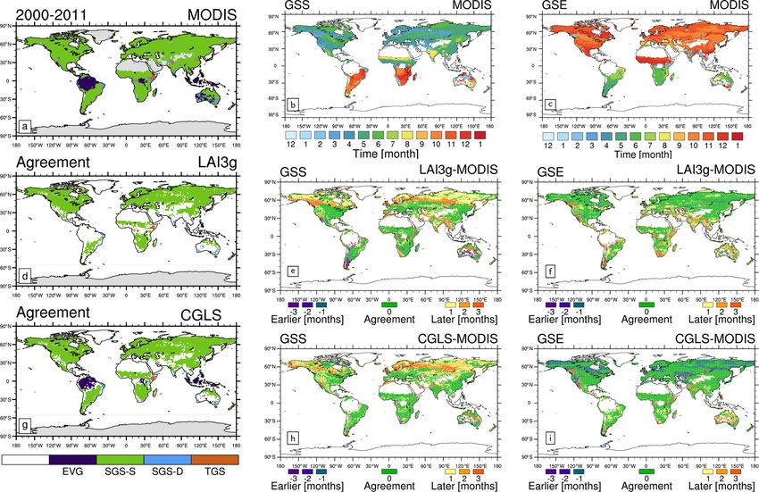
LSMs exhibit better agreement with MODIS GSS and ES (Sect. 2.2.3, 2.2.5 and Table 1). Similar to JULES-ES,
GSE timings in the NH compared to the SH (Figs. 4 and 5 JSBACH presents a small number of PFTs, but it reaches bet-
and Tables 3 and 4). Only CLM 5.0 and LPJ-GUESS show ter results thanks to the five implemented phenology schemes
similar results in both hemispheres (Table 3). In particular, (Sect. 2.2.4 and Table 1).
LPJ-GUESS shows good skill (agreement with observation The two Community Land Model versions (i.e. CLM4.5
larger than 15 %) in capturing both GSS and GSE timings in and CLM 5.0, Table 3) show very different outcomes, with
both hemispheres (Figs. 3f, 4f, and 5f). CLM5.0 exhibiting larger biases in GSS and GSE timings
LPJ-GUESS is the model that shows the highest agree- compared to CLM4.5 (Fig. 4b and c, Fig. 5b and c, and
ment with MODIS (Table 3) and the lowest bias in average Table 4). The two model versions differ in the crop rep-
GSS and GSE timings (0.4 and 0.1 months, respectively, Ta- resentation, plant physiology, and phenology parameteriza-
ble 4). JULES-ES shows the lowest agreement with MODIS tion (Sect. 2.2 and Table 1). The implementation of an an-
(Table 3) and the highest bias in the average GSS and GSE tecedent rain requirement trigger for stress-deciduous PFTs
timings (1.2 and −2.3, respectively, Table 4). This result (Dahlin et al., 2015) helps improved phenology in semi-arid
may be associated with the representation of PFTs in the regions (e.g. the sub-Sahara, Fig. 4b and c, and Fig. 5b and
two models used to describe global vegetation. LPJ-GUESS, c). Nonetheless, Zhang et al. (2019) show that the same up-
indeed, is the model featuring the largest number of PFTs, grade influences the leaf senescence in temperate grasslands.
while JULES-ES uses the least (Table 1). Moreover, JULES- On the other hand, the irrigation scheme in the CLM5.0
ES and LPJ-GUESS differ also on the details of the phenol- crop model allows for the improvement in crop-dominated
ogy parameterization. LPJ-GUESS features three phenology regions, such as the Indian subcontinent (Fig. 4b and c and
Biogeosciences, 18, 2405–2428, 2021 https://doi.org/10.5194/bg-18-2405-2021D. Peano et al.: Plant phenology evaluation of CRESCENDO LSMs – Part 1 2415
Figure 3. Global climatological (averaged over 2000–2011) distribution of the four main growing season modes for (a) MME, (b) CLM 4.5,
(c) CLM 5.0, (d) JULES-ES, (e) JSBACH, (f) LPJ-GUESS, (g) ORCHIDEE, and (h) ISBA-CTRIP. The areas characterized by the same type
of LSMs and MODIS (Fig. 2a) are coloured. These common areas are called agreement regions. Index values: (purple) evergreen, (green)
single season with summer LAI peak, (cyan) single growing season with summer dormancy, and (orange) two growing seasons type. White
regions are for disagreement areas. Above this selection, areas of agreement between satellite products are shaded with a different hatching
pattern: MODIS and LAI3g (Fig. 2d) slash hatching (/); MODIS and CGLS (Fig. 2g) backslash hatching (\); MODIS, CGLS, and LAI3g
crossed hatching (×).
Fig. 5b and c). Further differences occur between CLM 4.5 CGLS and LAI3g support the results obtained with
and CLM 5.0 (Fig. 4b and c and Fig. 5b and c), which could MODIS in the NH mid-latitude regions, Africa, and Brazil
be ascribed to the changes in plant physiology, soil hydrol- (shaded cross pattern in Figs. 4 and 5). Only LAI3g supports
ogy, and rooting profile. For example, CLM5.0 applies a dif- MODIS outcomes in the NH high-latitude regions (shaded
ferent rooting profile scheme and soil moisture threshold (Ta- slash pattern in Figs. 4 and 5). In general, the direct compar-
ble 1) affecting the representation of the soil moisture impact ison of LSMs with LAI3g and CGLS satellite observations
on phenology. exhibits results following MODIS ones (Figs. S5–S8 and Ta-
bles S3–S6).
https://doi.org/10.5194/bg-18-2405-2021 Biogeosciences, 18, 2405–2428, 20212416 D. Peano et al.: Plant phenology evaluation of CRESCENDO LSMs – Part 1
Figure 4. Global climatological (averaged over 2000–2011) differences in the growing season start timings (GSS) between (a) multi-model
ensemble mean (MME), (b) CLM 4.5, (c) CLM 5.0, (d) JULES-ES, (e) JSBACH, (f) LPJ-GUESS, (g) ORCHIDEE, and (h) ISBA-CTRIP
and MODIS (Fig. 2b). The green regions represent areas of agreement between MODIS and LSMs. Yellow-red colours correspond to areas
where models timings are later compared to MODIS, while blue-violet colours correspond to areas where models timings are previously
compared to MODIS. Regions where GSS timings are not computed, such as non-vegetated and evergreen areas, are in white. Above this
selection, areas of agreement between satellite products are shaded with a different hatching pattern: MODIS and LAI3g (Fig. 2d) slash
hatching (/); MODIS and CGLS (Fig. 2g) backslash hatching (\); MODIS, CGLS, and LAI3g crossed hatching (×). Note that the GSS in
the TGS regions corresponds to the GSS of the first growing season cycle.
3.4 Latitudinal variability ranges between −1.8 months (earlier GSS) just south of
the Equator and +2.0 months (delayed GSS) south of 50◦ S
The MME zonal average shown in Fig. 6 highlights the (Fig. 6a). The GSE bias ranges between −3.0 months in the
LSMs’ abilities and limitations in simulating the observed 0–10◦ N latitudinal band and +1.3 months in the southern
GSS and GSE timings at different latitudes. The GSS bias sub-tropics. The CRESCENDO LSMs correctly simulate the
Biogeosciences, 18, 2405–2428, 2021 https://doi.org/10.5194/bg-18-2405-2021D. Peano et al.: Plant phenology evaluation of CRESCENDO LSMs – Part 1 2417 Figure 5. As Fig. 4 but for growing season end (GSE) timings. Note that the GSE in the TGS regions corresponds to the GSE of the second growing season cycle. GSE timings north of 60◦ N. The Spearman correlation of that differences among satellite data also occur in the NH the GSS and GSE latitudinal distributions is 0.67 ± 0.07 and mid- and high-latitude regions, highlighting potential dif- 0.51 ± 0.11, respectively. These values are significant at the ferences among these three products (see Sect. 4.2). Large 95 % level based on a Monte Carlo approach. LSM biases in NH tropical region GSE timings and south- In the NH mid- and high-latitude regions, the LSMs’ GSS ern sub-tropical GSS timings are driven by premature val- timings exhibit an average delay of up to 1.6 months, espe- ues in Africa (Fig. S9c, d). These discrepancies may derive cially in North America (Fig. S9a). This bias and the spread from difficulties in the LSM’s ability to simulate the observed among LSMs might be driven by differences in tempera- phenology type and the response to soil moisture in Africa ture schemes and thresholds used by LSMs (Table 1). Note (Figs. 3 and S10). Large variability is spotted in the region https://doi.org/10.5194/bg-18-2405-2021 Biogeosciences, 18, 2405–2428, 2021
2418                                            D. Peano et al.: Plant phenology evaluation of CRESCENDO LSMs – Part 1

Table 4. Average difference between MODIS and LAI3g, CGLS, each land surface model, and multi-model ensemble mean (MME) in the
growing season start (GSS) and growing season end (GSE) timings. Values are reported in months for global, Northern Hemisphere (NH),
and Southern Hemisphere (SH). Positive values stand for later timings, and negative values correspond to earlier timings.

             LAI3g     CGLS     CLM 4.5     CLM 5.0    JULES-ES      JSBACH      LPJ-GUESS      ORCHIDEE       ISBA-CTRIP      MME
  GSS          0.25     0.30        0.54       0.81          1.23        0.35            0.37          0.64            0.44     0.56
  GSE         −0.16    −0.31       −0.30      −1.15         −2.26       −0.28            0.14         −0.10           −0.30    −0.49
  GSS NH       0.41     0.38        0.95       1.47          1.42        0.95            0.44          0.69            0.97     0.98
  GSE NH      −0.31    −0.48       −0.47      −1.69         −2.58       −0.69            0.10         −0.29           −0.59    −0.84
  GSS SH      −0.42    −0.01       −1.31      −2.18         −1.80       −2.48            0.11           0.41          −2.04    −1.23
  GSE SH       0.46     0.39        0.42       1.34          2.94        1.66            0.34           0.82           1.03     1.00

Figure 6. Zonal mean (a) growing season start (GSS) and (b) growing season end (GSE) timings for LAI3g (red lines), MODIS (green lines),
CGLS (blue lines), and multi-model ensemble mean (black dashed line). The grey regions show the multi-model ensemble spread. Values
are reported as month of the year (MOY), and the latitudinal coverage goes from 56◦ S to 75◦ N, which is the range covered by CGLS.

below 40◦ S. The reduced amount of vegetated land area may            3.5   Regional variability
cause this behaviour. A different growing season type detec-
tion in this area, such as a different size of the evergreen re-      To assess sources of biases in the LSMs, different biomes
gion (Fig. 2), may, indeed, extensively influence the GSS and         derived from the ESA CCI land cover map (Li et al., 2018,
GSE detection, which is the case for the satellite products           Fig. 7a) are investigated. The GSS timings are generally de-
(Fig. 6), especially LAI3g.                                           layed compared to observations, except for the broadleaf ev-
   Observed latitudinal distributions highlight an increas-           ergreen tree (BET) and broadleaf deciduous shrub (BDS)
ing northward trend in the NH mid-latitude GSE timings                biomes (Fig. 7f, k). In BDS-dominated regions, the multi-
(GSE around May–June at ∼ 20◦ N and around September–                 model ensemble mean (MME) falls within the observational
October at ∼ 40◦ N, Fig. 6b) and an increasing southward              range (Fig. 7f, k), but a large spread among LSMs exists.
trend in the 30–55◦ S latitudinal band (GSS around July at            The BDS-dominated regions are semi-arid and transition ar-
∼ 30◦ S and around September at ∼ 55◦ S, Fig. 6a). Similar            eas, where LSMs’ parameterization could be more sensi-
trends are reproduced by the LSMs, but with a higher mag-             tive to climate conditions and parameter selection, especially
nitude (Fig. 6). In the NH, the difference between simulated          soil moisture. The large spread among LSMs, then, might
and observed trends may be driven by an overestimated in-             be mostly linked to the differences in the implementation of
fluence of radiation and temperature on leaf senescence in            soil moisture in the phenology schemes (Table 1). It is note-
LSMs. In the SH, the discrepancies between observed and               worthy that this biome covers a small fraction of the global
modelled trends may be related to relatively large phenology          vegetated regions. The largest biome (i.e. Grass in the North-
variability in the SH associated with the small vegetated land        ern Hemisphere, Fig. 7g) instead exhibits a mean delay of
area in this hemisphere.                                              1 month, which is common among the LSMs except for LPJ-
                                                                      GUESS, which falls within observed range. Besides, large
                                                                      biome variability is visible in the SH Crop biome (Fig. 7m).

Biogeosciences, 18, 2405–2428, 2021                                                       https://doi.org/10.5194/bg-18-2405-2021
D. Peano et al.: Plant phenology evaluation of CRESCENDO LSMs – Part 1 2419
In general, LSMs show a larger variability in the South- agreement in the NH (Table 3). High skill (agreement with
ern Hemisphere (SH) compared to the Northern Hemisphere observation larger than 20 % for at least one timing) in the
(NH). NH is obtained by CLM4.5, ORCHIDEE, and ISBA-CTRIP
GSE timings display heterogeneous outcomes (Fig. 8). In (Table 3). The different performance between models can oc-
general, a larger variability is observed compared to GSS cur from differences in phenology parameterization as well
timings. The NH Grass biome, which covers about 33 % of as different vegetation cover types (plant and crop functional
the global vegetated area, exhibits a mean delay of 1 month types), soil characterization, and initial spatial resolution (Ta-
which is mainly driven by JULES-ES (Fig. 8g). The SH ble 1).
BDS area displays a large variability among models (Fig. 8k) Among the LSMs evaluated here, JULES-ES shows rela-
ranging from May (LPJ-GUESS) to November (JULES- tively lower skill in simulating GSS and GSE timings com-
ES). Large biome variability appears in broadleaf evergreen pared to the other LSMs (Table 3). This result may be as-
tree (BET), Grass and Crop SH biomes (Fig. 8i, l, m), and cribed to the smaller number of PFTs (see Table 1) and de-
NH Crop (Fig. 8h). This result highlights the need for fur- tails of the phenology parameterization that characterize this
ther investigation on the representation of crop phenology LSM (Sect. 2.2.3 and Table 1). JSBACH accounts for a sim-
in the LSMs since only a few LSMs (i.e. JSBACH and ilar number of PFTs (Table 1) but features a more complex
ORCHIDEE) treat crops with a specific parameterization phenology scheme (Sect. 2.2.4 and Table 1). For this reason,
(Sect. 2). JSBACH exhibits a higher skill than JULES-ES in reproduc-
In general, LSMs show a higher agreement in representing ing GSS and GSE timings (Table 3).
GSS timings compared to GSE timings. Consequently, the Similar to JSBACH, ORCHIDEE features a PFT-oriented
different approaches used to describe the start of the growing phenology scheme (Sect. 2.2.6 and Table 1), which con-
season are relatively consistent among LSMs. In comparison, tributes to the high skill noted for ORCHIDEE.
the representation of the end of the vegetative season requires CLM 4.5, CLM 5.0, and LPJ-GUESS use three phenology
further investigation and development. Note that this regional schemes: (1) evergreen, (2) seasonal deciduous, and (3) stress
evaluation is performed based on the observed biome distri- deciduous (Sect. 2.2.1, 2.2.2, 2.2.5). Among these schemes,
bution (i.e. ESA CCI map). However, each LSM treats dif- the seasonal deciduous one employs calendar thresholds
ferently the land cover and biome distribution (Sect. 2). For (summer and winter solstices and day length threshold in
this reason, part of the obtained spread among LSMs de- CLM, and fixed 210 d phenology in LPJ-GUESS) that may
rives from differences in PFT representation and distribution improve the results of LPJ-GUESS and CLM 4.5. On the
(Sect. 2.2, and Table 1), which affect phenology representa- other hand, this may mean that the seasonal-deciduous type
tion in LSMs. may be less responsive to future climate change.
Contrary to the other LSMs, ISBA-CTRIP uses the daily
leaf carbon balance to simulate plant phenology, and it
4 Discussion reaches good skill (Tables 3, 4). Consequently, ISBA-CTRIP
highlights the opportunity to attain results aligned with the
4.1 Land surface models other LSMs using leaf carbon availability instead of climatic
conditions.
The plant phenology growing season start and end are mainly The improvement of the phenology parameterization can
triggered by changes in solar radiation, temperature, and soil lead to better representation of vegetation in the LSMs. How-
moisture conditions (e.g. Caldararu et al., 2012; Zeng et al., ever, other vegetation features affect the plant phenology
2013; Tang and Dubayah, 2017). State-of-the-art LSMs rep- representation, as in the case of the two CLM versions.
resent the phenological transitions using different parameter- CLM4.5 and CLM5.0 share similar phenology parameteri-
izations based on the climate conditions (Sect. 2.2). Many zation (Sect. 2.2.1 and 2.2.2) but differ in the crop irrigation
of these parameterizations (see Sect. 2.2) are based on val- scheme, soil and plant hydrology, and carbon and nitrogen
ues derived from localized observations (e.g. White et al., cycling (Lawrence et al., 2018). Since soil moisture has a
1997; Thornton et al., 2002; Jolly et al., 2005; Savoy and significant control on plant phenology (e.g. Caldararu et al.,
Mackay, 2015). Consequently, the phenology parameters are 2012), the CLM5.0 revision of stomatal response to rising
calibrated on specific regions of the globe, which may be one CO2 concentrations through a new Medlyn stomatal con-
reason for the large spread of values seen in the present anal- ductance scheme (Fisher et al., 2019; Medlyn et al., 2011)
ysis. and the use of a revised mechanistically based soil evapora-
Generally, phenology calibration areas are located in the tion parameterization that accounts for the rate of diffusion
NH, where LSMs exhibit better results and larger coherence of water vapour through a dry surface layer (Swenson and
compared to the SH. Among the LSMs evaluated here, LPJ- Lawrence, 2014) are likely to be principal sources of differ-
GUESS, CLM4.5, and ORCHIDEE show good skill (agree- ences between CLM5.0 and CLM4.5.
ment with observation larger than 15 %) in the SH (Table 3).
On the other hand, CLM5.0 and JULES-ES do not reach such
https://doi.org/10.5194/bg-18-2405-2021 Biogeosciences, 18, 2405–2428, 2021You can also read