Multi-decadal hydrologic change and variability in the Amazon River basin: understanding terrestrial water storage variations and drought ...
←
→
Page content transcription
If your browser does not render page correctly, please read the page content below
Hydrol. Earth Syst. Sci., 23, 2841–2862, 2019
https://doi.org/10.5194/hess-23-2841-2019
© Author(s) 2019. This work is distributed under
the Creative Commons Attribution 4.0 License.

Multi-decadal hydrologic change and variability in the Amazon
River basin: understanding terrestrial water storage variations
and drought characteristics
Suyog Chaudhari1 , Yadu Pokhrel1 , Emilio Moran2 , and Gonzalo Miguez-Macho3
1 Department of Civil and Environmental Engineering, Michigan State University, East Lansing, MI 48824, USA
2 Department of Geography, Environment and Spatial Sciences, Michigan State University, East Lansing, MI 48824, USA
3 Non-Linear Physics Group, Faculty of Physics 15782, Universidade de Santiago de Compostela, Galicia, Spain

Correspondence: Yadu Pokhrel (ypokhrel@egr.msu.edu)

Received: 4 February 2019 – Discussion started: 13 February 2019
Accepted: 7 June 2019 – Published: 8 July 2019

Abstract. We investigate the interannual and interdecadal        ing climate and increasing hydrologic alterations due to hu-
hydrological changes in the Amazon River basin and its sub-      man activities (e.g., LULC change).
basins during the 1980–2015 period using GRACE satellite
data and a physically based, 2 km grid continental-scale hy-
drological model (LEAF-Hydro-Flood) that includes a prog-
nostic groundwater scheme and accounts for the effects of        1   Introduction
land use–land cover (LULC) change. The analyses focus
on the dominant mechanisms that modulate terrestrial water       The Amazon River basin is one of the most hydrologi-
storage (TWS) variations and droughts. We find that (1) the      cally and ecologically diverse regions in the world (Fan and
model simulates the basin-averaged TWS variations remark-        Miguez-Macho, 2010; Latrubesse et al., 2017; Lenton et al.,
ably well; however, disagreements are observed in spatial        2009; Lesack, 1993; Malhi et al., 2008; Moran et al., 2018;
patterns of temporal trends, especially for the post-2008 pe-    Timpe and Kaplan, 2017; Tófoli et al., 2017). It is home to
riod. (2) The 2010s is the driest period since 1980, charac-     the world’s largest tropical rainforest and hosts ∼ 25 % of all
terized by a major shift in the decadal mean compared to the     terrestrial species on Earth (Malhi et al., 2008). Hydrologi-
2000s caused by increased drought frequency. (3) Long-term       cally, it contributes to 20 %–30 % of the world’s total river
trends in TWS suggest that the Amazon overall is getting         discharge into the oceans (Clark et al., 2015; Muller-Karger
wetter (1.13 mm yr−1 ), but its southern and southeastern sub-   et al., 1988; Nepstad et al., 2008) and accounts for ∼ 15 % of
basins are undergoing significant negative TWS changes,          global terrestrial evapotranspiration (Field et al., 1998; Malhi
caused primarily by intensified LULC changes. (4) Increas-       et al., 2008). Thus, the Amazon is an important component of
ing divergence between dry-season total water deficit and        global terrestrial ecosystems and the hydrologic cycle (Cox
TWS release suggests a strengthening dry season, especially      et al., 2004; Nobre et al., 1991); it also plays a major role
in the southern and southeastern sub-basins. (5) The sub-        in global atmospheric circulation through precipitation recy-
surface storage regulates the propagation of meteorological      cling and atmospheric moisture transport (Malhi et al., 2008;
droughts into hydrological droughts by strongly modulating       Soares-Filho et al., 2010).
TWS release with respect to its storage preceding the drought       The hydro-ecological systems of the Amazon are depen-
condition. Our simulations provide crucial insight into the      dent on plentiful rainfall (Cook et al., 2012; Espinoza et al.,
importance of sub-surface storage in alleviating surface wa-     2015, 2016; Espinoza Villar et al., 2009; Nepstad et al., 2008)
ter deficit across Amazon and open pathways for improving        and the vast amount of water that flows down through ex-
prediction and mitigation of extreme droughts under chang-       tensive river networks and massive floodplains (Bonnet et
                                                                 al., 2008; Coe et al., 2002; Frappart et al., 2011; Miguez-

Published by Copernicus Publications on behalf of the European Geosciences Union.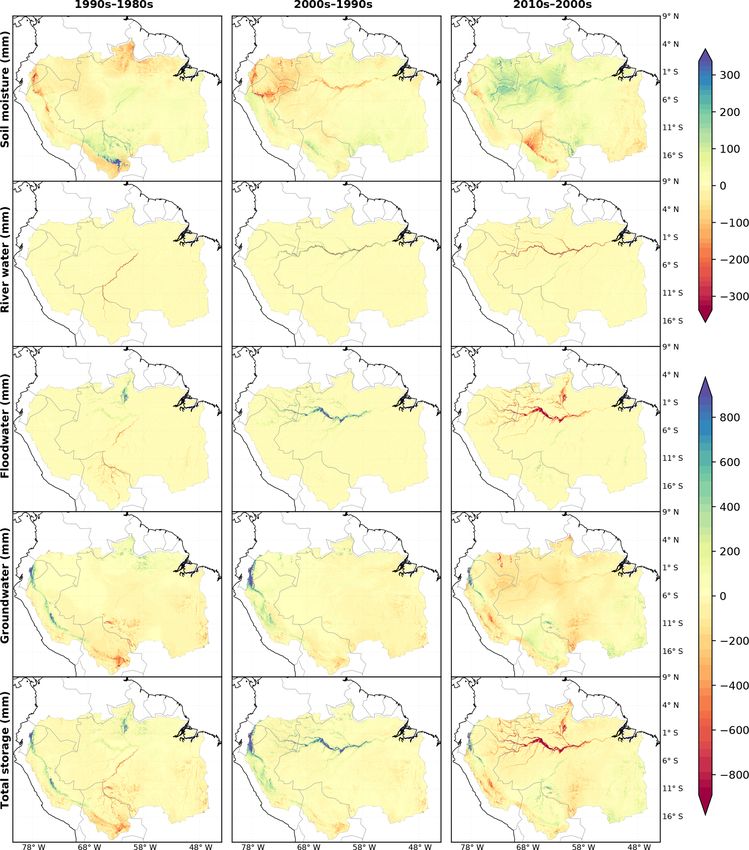
2842                                                   S. Chaudhari et al.: Multi-decadal hydrologic change and variability

Macho and Fan, 2012a; Yamazaki et al., 2011; Zulkafli et al.,     et al., 2011; Phillips et al., 2009; Saleska et al., 2007, 2016;
2016). The spatiotemporal patterns of precipitation are, how-     Satyamurty et al., 2013; Schöngart and Junk, 2007; Xu et al.,
ever, changing due to climate change and variability (Brando      2011; Zeng et al., 2008). For example, Lewis et al. (2011)
et al., 2014; Cook et al., 2012; Lima et al., 2014; Malhi et      found that the 2010 drought was spatially more extensive
al., 2008, 2009; Nepstad et al., 2008), large-scale alterations   than the 2005 drought; the spatial extent was over 3.0 mil-
in land use (e.g., deforestation) (Chen et al., 2015; Coe et      lion square kilometers in 2010 and 1.9 million square kilo-
al., 2009; Davidson et al., 2012; Kalamandeen et al., 2018;       meters in 2005. These catastrophic droughts had major im-
Lima et al., 2014; Panday et al., 2015; Tollefson, 2016),         plications on the hydrology of the Amazon River basin; for
and more recently the construction of mega-dams (Finer and        example, the 2005 hydrological drought led to reduction in
Jenkins, 2012; Latrubesse et al., 2017; Moran et al., 2018;       streamflow by 32 % from the long-term mean, as reported in
Soito and Freitas, 2011; Timpe and Kaplan, 2017; Wine-            Zeng et al. (2008), and in 2010 moisture stress induced per-
miller et al., 2016), among others. Such changes in precipita-    sistent declines in vegetation greenness affecting an area of
tion patterns typically manifest themselves in terms of altered   ∼ 2.4 million square kilometers, which was 4 times greater
magnitude, duration, and timing of streamflow (Marengo,           than the area impacted in 2005 (Xu et al., 2011). Moreover,
2005). A prominent streamflow alteration pattern that has         these extreme drought events, coupled with forest fragmenta-
been widely observed across the Amazon is the extended dry-       tion, have caused widespread fire-induced tree mortality and
season length (Espinoza et al., 2016; Marengo et al., 2011)       forest degradation across Amazonian forests (Aragão et al.,
and an increase in the number of dry events (i.e., droughts)      2007; Brando et al., 2014; Davidson et al., 2012; Malhi et al.,
over the longer term (Malhi et al., 2009; Marengo and Es-         2008; Rammig et al., 2010).
pinoza, 2016), which has been suggested to be a result of            Due to the limited availability of observed data (e.g., pre-
ongoing climatic and human-induced changes (Cook et al.,          cipitation, streamflow) for the entire basin, hydrologic char-
2012; Cook and Vizy, 2008; Lee et al., 2011; Malhi et al.,        acteristics of droughts in the Amazon have been studied pri-
2008; Shukla et al., 1990). However, the cross-scale interac-     marily by using hydrological models and satellite remote
tions and feedbacks in the human–water relationship make          sensing. For example, early studies (Coe et al., 2002; Costa
it difficult to explicitly quantify the causes. These changes     and Foley, 1999; Lesack, 1993; Vorosmarty et al., 1996;
have resulted in decreases in runoff (Espinoza et al., 2009;      Zeng, 1999) examined different components of the Amazon
Haddeland et al., 2014; Lima et al., 2014) and loss of ter-       water budget and their trends through relatively simpler mod-
restrial biodiversity (Barletta et al., 2010; Newbold et al.,     els. More recent literature (Dias et al., 2015; Fan et al., 2019;
2016; Tófoli et al., 2017; Toomey et al., 2011; Winemiller        Getirana et al., 2012; Miguez-Macho and Fan, 2012a, b;
et al., 2016). Increased variability in streamflow has also re-   Paiva et al., 2013a, b; Pokhrel et al., 2012a, b, 2013; Shin et
sulted in the disruption of the food pulse and fishery yields,    al., 2018; Siqueira et al., 2018; Wang et al., 2019; Yamazaki
which the Amazon region thrives upon (Castello et al., 2013,      et al., 2011, 2012) provided further advances in modeling the
2015; Forsberg et al., 2017). Moreover, persistent dry events     hydrological dynamics connected with anthropogenic activ-
create negative social externalities, such as deterioration of    ities in the Amazon and other parts of the world. Methods
respiratory health due to drought-induced fires (Smith et al.,    with varying complexities were used in similar studies, rang-
2014), exhaustion of family savings (Brondizio and Moran,         ing from simple water budget analyses (Betts et al., 2005;
2008), and isolation of communities that are affected by river    Costa and Foley, 1999; Fernandes et al., 2008; Lesack, 1993;
navigation and drinking water scarcity (Sena et al., 2012),       Sahoo et al., 2011; Vorosmarty et al., 1996; Zeng, 1999) to
hence affecting the overall livelihood of the local communi-      state-of-the-art land surface models (Getirana et al., 2012;
ties. Thus, it is critical to understand the characteristics of   Miguez-Macho and Fan, 2012a, b; Paiva et al., 2013a, b;
historical droughts to better understand the dominant mech-       Pokhrel et al., 2013; Siqueira et al., 2018; Wongchuig Correa
anisms that modulate droughts and their evolution over time.      et al., 2017; Yamazaki et al., 2011, 2012), with some target-
   As often is the case, droughts in the Amazon are driven        ing the overall development of parameterization and process
by El Niño events; however, some droughts are suggested           representation in the model (Coe et al., 2008, 2009; Dias et
to be caused by climate change and variability (Espinoza et       al., 2015; Getirana et al., 2010, 2012, Miguez-Macho and
al., 2011; Lewis et al., 2011; Marengo et al., 2008; Marengo      Fan, 2012a, b; Paiva et al., 2013b; Pokhrel et al., 2013; Ya-
and Espinoza, 2016; Phillips et al., 2009; Xu et al., 2011;       mazaki et al., 2011) and others focusing on the hydrologi-
Zeng et al., 2008) and due to accelerating human activi-          cal changes occurring in the basin due to weather variability
ties causing rapid changes in the land use and water cycle        (Coe et al., 2002; Lima et al., 2014; Wongchuig Correa et al.,
(Lima et al., 2014; Malhi et al., 2008). Numerous studies         2017).
have quantified the impacts and spatial extent of these peri-        Major drought events in the Amazon, particularly those
odic droughts on the hydrological and ecological systems in       in recent years, have been detected by satellite remote sens-
the Amazon (Alho et al., 2015; Brando et al., 2014; Castello      ing, and their impacts on terrestrial hydrology have been ex-
et al., 2013, 2015, Chen et al., 2009, 2010; da Costa et al.,     amined (Chen et al., 2010; Filizola et al., 2014; Xu et al.,
2010; Davidson et al., 2012; Fernandes et al., 2011; Lewis        2011). In particular, the hydrologic impact of droughts has

Hydrol. Earth Syst. Sci., 23, 2841–2862, 2019                                   www.hydrol-earth-syst-sci.net/23/2841/2019/
S. Chaudhari et al.: Multi-decadal hydrologic change and variability                                                        2843

been revealed by examining the anomalies in terrestrial water     as to anticipate future hydrological conditions (Phipps et al.,
storage (TWS) inferred from the Gravity Recovery and Cli-         2013). Many aspects of the droughts are yet to be studied,
mate Experiment (GRACE) satellites. A significant decrease        such as, the interdependence between TWS and meteoro-
in TWS over Central Amazon in the summer of 2005, rela-           logical (precipitation-related) and hydrological (streamflow-
tive to the average of the five other summer months during        related) droughts. A complete categorization of the drought
the 2003–2007 period, was reported by Chen et al. (2009).         events with respect to their causes and impacts and the re-
However, due to the vast latitudinal extent of the Amazon         sulting basin response is still coming up short.
basin, these severe dry conditions were observed only in             In this study, we investigate the interannual and inter-
some regions of the basin. Xavier et al. (2010) and Frap-         decadal variability in TWS and drought events in the Ama-
part et al. (2013) used GRACE TWS estimates to identify           zon River basin over 1980–2015 period. Our study is driven
the signature of these drought events and suggested that the      by the following key science questions: (1) how do interan-
2005 drought only affected the western and central parts          nual and interdecadal changes in drought conditions mani-
of the basin, whereas very wet conditions peaking in mid-         fest as long-term variations in TWS at varying spatial and
2006 were observed in the eastern, northern, and southern         temporal scales in the Amazon River basin? (2) What are
regions of the basin. Although the ramifications of these ex-     the impacts of TWS variations on dry-season water deficit
treme droughts have been widely studied using remote sens-        and release? Is the Amazonian dry season getting stronger
ing datasets (e.g., GRACE), the understanding of their time       or more severe? (3) What are the dominant factors driving
evolution is limited due to data gaps and short study periods,    the evolution of TWS and drought conditions at varying spa-
hence hindering their comprehensive categorization. Further,      tial and temporal scales? (4) How does the sub-surface water
GRACE provides the changes in vertically integrated TWS           storage regulate the water deficiency caused by the surface
variations; thus variations in the individual TWS components      drought conditions? These questions are answered by using
cannot be estimated solely by GRACE. This shortcoming is          hydrological simulations from a continental-scale hydrolog-
overcome by using hydrological models that separate TWS           ical model and the TWS data from GRACE satellites; the
into its individual components and provide simulations for        goal is to provide a comprehensive picture of characteris-
an extended timescale. However, discrepancy between mod-          tics and evolution of droughts in the Amazon with respect
els and GRACE observations has also become a major topic          to their types and spatial impact. Specifically, this study aims
of discussion, as most of the global models show an oppo-         to (i) examine the impacts of drought conditions on TWS and
site trend in TWS compared to GRACE in the Amazon and             other hydrological variables, (ii) understand the hydrological
other global river basins (Scanlon et al., 2018); yet, no clear   variability and drought evolution in the Amazon at an annual
explanation or quantification exists in the published litera-     and decadal scale over the past four decades, (iii) quantify
ture, apart from the attribution of the discrepancy to model      the role of sub-surface water storage in alleviating the sur-
shortcomings (see Sect. 3.3 for details).                         face drought conditions, and (iv) summarize each drought
   As referenced above, the changing hydroclimatology of          year by providing a comprehensive characterization for the
the Amazon basin, along with specific drought-related anal-       major drought events in the Amazon and its sub-basins.
ysis (e.g., 2005, 2010), has been widely reported in a large
body of literature published over recent decades. Several
studies have used statistical measures to quantify drought        2     Model and data
severity (Espinoza et al., 2016; Gloor et al., 2013; Joetzjer
et al., 2013; Marengo, 2006; Marengo et al., 2008, 2011;          2.1    The LEAF-Hydro-Flood (LHF) model
Wongchuig Correa et al., 2017; Zeng et al., 2008; Zhao et al.,
2017a), concerning common variables, such as streamflow           The model used in this study is LHF (Fan et al., 2013;
and precipitation, thus limiting the quantification of drought    Miguez-Macho and Fan, 2012a, b; Pokhrel et al., 2013,
impact on water stores, viz. flood, groundwater, and TWS.         2014), a continental-scale land hydrology model that re-
Further, even though these studies encompass different as-        solves various land surface hydrologic and groundwater pro-
pects of hydrological and climatic changes, most span only a      cesses on a full physical basis. It is derived from the model
few years to a decade, except for some precipitation-related      Land Ecosystem–Atmosphere Feedback (LEAF) (Walko et
studies (Marengo, 2004; Marengo et al., 1998). Other studies      al., 2000), the land surface component of the Regional At-
have used a relatively longer study period (Costa et al., 2003;   mosphere Modeling System (RAMS) (Pielke et al., 1992).
Espinoza et al., 2016; Zeng, 1999), but the spatial extent is     The original LEAF was extensively improved and enhanced
limited. Thus, a comprehensive understanding of the inter-        to develop LEAF-Hydro for North America (Fan et al., 2007;
decadal hydrologic change and variability across the entire       Miguez-Macho et al., 2007) by adding a prognostic ground-
basin and that of changes in drought characteristics is still     water storage and allowing (1) the water table to rise and
lacking. Given the number of droughts that have occurred          fall or the vadose zone to shrink or grow; (2) the water
and their widespread impact in the Amazon, it is impera-          table, recharged by soil drainage, to relax through stream-
tive to have a better understanding of these past events so       flow into rivers, and lateral groundwater flow, leading to

www.hydrol-earth-syst-sci.net/23/2841/2019/                                    Hydrol. Earth Syst. Sci., 23, 2841–2862, 2019
2844                                                 S. Chaudhari et al.: Multi-decadal hydrologic change and variability

convergence to low valleys; (3) two-way exchange between        (1992–1999), SPOT-Vegetation (1999–2012), and PROBA-
groundwater and rivers, representing both losing and gaining    V (2013–2015) instruments. The classification follows the
streams; (4) river routing to the ocean as kinematic waves;     LULC classes defined by the UN Land Cover Classification
and (5) setting sea level as the groundwater head bound-        System (LCCS). Spatiotemporal coverage and resolution of
ary condition. Miguez-Macho and Fan (2012a) further en-         these LULC maps are consistent with the specific LHF model
hanced the LEAF-Hydro framework by incorporating the            requirements; hence we use annual land cover input, spatially
river–floodplain routing scheme which solves the full mo-       aggregated to 2 km LHF model grids, following the general
mentum equation of open-channel flow, giving more realistic     practice in hydrologic impact studies (Arantes et al., 2016;
streamflow estimates by considering the prominent backwa-       Panday et al., 2015).
ter effect observed in the Amazon (Bates et al., 2010; Ya-         Because the ESA-CCI data did not cover the simulation
mazaki et al., 2011). The LHF model has been extensively        period prior to year 1992, we derive the time series products
validated in the North and South American continents on 5       for the 1980–1991 period by using the trend in leaf area index
and 2 km grids, respectively (Fan et al., 2013; Miguez-Macho    (LAI) and the ESA-CCI land cover map for year 1992 as a
et al., 2008; Miguez-Macho and Fan, 2012a, b; Pokhrel et al.,   baseline. A pixel-by-pixel analysis is conducted, and the pix-
2013; Shin et al., 2018) and used to examine the impacts of     els with mean annual LAI higher than 5 are transitioned into
climate change on the groundwater system in the Amazon          the forest canopy, whereas for other pixels the LULC type
(Pokhrel et al., 2014). A complete description of LHF can be    is retained from the previous year’s LULC map. The thresh-
found in Miguez-Macho and Fan (2012a).                          old of LAI equal to 5 for facilitating the land cover transi-
                                                                tion into forest is determined based on the LAI classifications
2.2    Atmospheric forcing                                      provided in past literature (Asner et al., 2003; Myneni et al.,
                                                                2007; Xu et al., 2018). Reverse prediction of LULC changes
Atmospheric forcing data are taken from WATCH Forcing           was constrained to the forest canopy only, as it is difficult to
Data methodology applied to ERA-Interim reanalysis data         predict the LULC type based on LAI values less than 5. Also,
(WFDEI) (Weedon et al., 2014), available for the 1979–          forest cover is known to be the most prominent land cover in
2016 period at 0.5◦ spatial resolution and 3 h time steps.      the Amazon; hence it is reasonable to assume that most of the
The WFDEI dataset is widely used in both global- and            LULC changes occurring in the basin are transitioned from
regional-scale studies (Beck et al., 2016; Felfelani et al.,    forest cover.
2017; Hanasaki et al., 2018; Müller Schmied et al., 2014)          Monthly LAI data are derived by temporally aggregat-
and has been suggested to represent the observations in the     ing the 8 d composites from the Global Land Surface Satel-
Amazon region well (Monteiro et al., 2016). The original        lite (GLASS) LAI product (Liang and Xiao, 2012; Xiao et
WFDEI data at 0.5◦ resolution are spatially interpolated us-    al., 2014) to monthly values for the entire model domain.
ing a bilinear interpolation method to model grid resolution    GLASS LAI values for the period of 1982–1999 are derived
(∼ 2 km), following our previous studies (Miguez-Macho          from AVHRR reflectance, whereas MODIS reflectance val-
and Fan, 2012a, b; Pokhrel et al., 2013, 2014; Shin et al.,     ues are used for the period 2000–2012. Because of the data
2018). The more recent European Centre for Medium-Range         constraint, LAI data for the years before 1982 and after 2012
Weather Forecasts Reanalysis 5th (ERA5) dataset, which          are assumed to be the same as that of the years 1982 and
provides atmospheric forcing data from 1979 to present day      2012, respectively.
at a spatial resolution of 0.25◦ , shows promise by outper-
forming its predecessors (Towner et al., 2019). However, as     2.4     Validation data
no studies existed in the past literature which comprehen-
sively validated the ERA5 dataset over the Amazon region        2.4.1    Observed streamflow
until recently, WFDEI forcing remains a better alternative as
a model input.                                                  We use monthly averaged streamflow data obtained from
                                                                the Agência Nacional de Águas (ANA) in Brazil (http://
2.3    Land use–land cover and leaf area index                  hidroweb.ana.gov.br, last access: 24 June 2019). A total of 55
                                                                stream gauge stations are selected considering a wide cover-
The land cover data used in this study are obtained from        age over the Amazonian sub-basins and a good balance be-
the European Space Agency Climate Change Initiative’s           tween low and high flow values. The major selection criterion
Land Cover project (ESA-CCI; http://maps.elie.ucl.ac.be/        is the data length; i.e., we only include gauges with at least
CCI/, last access: 24 June 2019). The data comprise an an-      30 years’ coverage. In a few cases, such as for the Japura sub-
nual time series of high-resolution land cover maps for the     basin, the threshold was overlooked because this criterion re-
1992–2015 period at a 300 m spatial resolution, generated by    sulted in a small number of gauging stations. All the selected
combining the baseline map from the Medium-spectral Res-        stations have observational data for varying time frames with
olution Imaging Spectrometer (MERIS) instrument and the         minimal data gaps; the months with missing data are skipped
land use–land cover (LULC) changes detected from AVHRR          in the statistical analysis.

Hydrol. Earth Syst. Sci., 23, 2841–2862, 2019                                  www.hydrol-earth-syst-sci.net/23/2841/2019/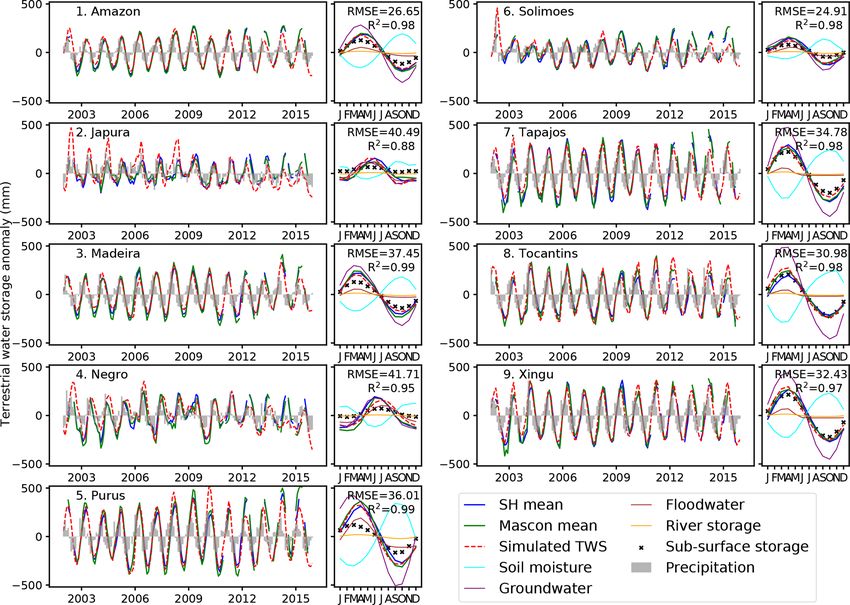
S. Chaudhari et al.: Multi-decadal hydrologic change and variability                                                         2845

2.4.2    GRACE data                                               whether the variable is below the threshold, expressed math-
                                                                  ematically as
The TWS products from the GRACE satellite mission are
                                                                                1 for Q(t, x) < Q90 (t, x)
used to validate the TWS simulated by LHF for the 2002–           Ds(t, x) =                                 ,             (2)
                                                                                0 for Q(t, x) ≥ Q90 (t, x)
2015 period. Equivalent water height from three process-
ing centers, namely (i) the Jet Propulsion Laboratory (JPL),      where Ds(t, x) indicates whether the grid (x) is in a drought
(ii) the Center for Space Research (CSR), and (iii) the Ger-      state at time (t), Q(t, x) is the streamflow, and Q90 (tx) is the
man Research Center for Geoscience (GFZ) (http://grace.jpl.       threshold for grid (x) at time (t). Consecutive drought states
nasa.gov/data/get-data/, last access: 24 June 2019) (Landerer     are added to get the drought duration. Events with duration
and Swenson, 2012), is used along with two mascon prod-           less than 3 d are not considered as droughts. The number of
ucts from CSR and JPL; mascon products have been sug-             drought days per year is calculated by aggregating the dura-
gested to better capture TWS signals in many regions (Scan-       tion of all the drought events in a year.
lon et al., 2016). Basin-averaged data of variation in TWS
anomalies are calculated from GRACE by taking an area-            2.7   Dry-season total water deficit
weighted arithmetic mean with varying cell area (Felfelani et
                                                                  We define the dry-season total water deficit (TWD) as the
al., 2017).
                                                                  cumulative difference between monthly potential evapotran-
2.5     TWS drought severity index                                spiration (PET) and precipitation (P ) for the period during
                                                                  which P < PET. The corresponding drop in the simulated
To examine the occurrence and severity of hydrological            TWS, during the same period as of TWD, is defined as the
droughts over the past decades, we employ the drought             TWS release (TWS-R). TWD and TWS-R can be conceptu-
severity index derived from time-varying TWS change from          alized as the annual water demand and supply as described
GRACE, known as the GRACE drought severity index                  in Guan et al. (2015). PET estimated at the daily interval us-
(GRACE-DSI) (Zhao et al., 2017b). We apply the GRACE-             ing the Penman–Monteith approach (Monteith, 1965) as in
DSI framework to the 36-year simulated TWS (hereafter re-         Pokhrel et al. (2014) is aggregated to the monthly scale to
ferred to as TWS-DSI) to examine the interannual and inter-       calculate TWD; for consistency, we use the WFDEI forc-
decadal drought evolution over the entire basin. This index       ing data that are used for LHF simulations (Sect. 2.2). TWS
is solely based on the TWS anomalies and has been shown           anomalies required for the estimation of storage release are
to capture the past droughts with favorable agreement with        obtained from the LHF model.
other drought indices derived from precipitation (e.g., PDSI
and SPEI) (Zhao et al., 2017a, b). TWS-DSI is calculated for      2.8   Simulation setup
each grid cell in the model domain as follows:
                                                                  LHF is set up for the entire Amazon basin (∼ 7.1 million
                TWSi,j − TWSj                                     square kilometers) including the Tocantins River basin. Sim-
TWS_DSIi,j    =               ,                            (1)
                      σj                                          ulations are conducted for the 1979–2015 period at a spa-
where TWSi,j is the TWS anomaly from LHF for year i and           tial resolution of 1 arcmin (∼ 2 km). The model time step
month j ; and TWSj and σj are the temporal mean and stan-         is 4 min as in previous studies (Miguez-Macho and Fan,
dard deviation of TWS anomalies for month j , respectively.       2012a, b; Pokhrel et al., 2013, 2014); however, model output
                                                                  is saved at daily time steps. To stabilize water table depth,
2.6     Occurrence and duration of drought                        the model is spun up for ∼ 150 years, starting with the equi-
                                                                  librium water table (Fan et al., 2013) for 1979, and results
The characteristics of hydrological droughts are identified       for the 1980–2015 period (36 years) are analyzed. As this
from the simulated streamflow using the widely used thresh-       study aims to analyze the hydrological changes in the Ama-
old level approach. Different thresholds have been proposed       zon on a decadal scale, simulations for 1979 are considered
in previous studies: mean flow, minimum and maximum               as additional spin-up and hence not used. Dynamic monthly
flows (Marengo and Espinoza, 2016; Wongchuig Correa et            LAI and annual LULC maps are used to account for LULC
al., 2017), 80th percentile (Q80 ) flow (Van Loon et al., 2012;   changes (see Sect. 2.3). Moreover, as the model simulates
Van Loon and Laaha, 2015; Wanders and Van Lanen, 2015),           land surface, hydrologic, and groundwater processes on a
and 90th percentile (Q90 ) flow (Wanders et al., 2015; Wan-       complete physical basis, no calibration was performed on
ders and Wada, 2015). In this study, we use Q90 , which is de-    the model output. The original novelty of the LHF model
rived from the flow duration curve, where Q90 is the stream-      framework, combined with the incorporated dynamic hu-
flow that is equaled or exceeded for 90 % of the time. Q90        man role through land cover change, creates a state-of-the-
is used to isolate severe drought events over the simulation      art framework for assessing long-term hydrological changes.
period. Monthly threshold values are derived using the 36-        The complete LHF framework along with the input data em-
year simulated streamflow and are smoothed by a 30 d mov-         ployed in this study are presented in Fig. S1 in the Supple-
ing average. Drought condition is identified by determining       ment.

www.hydrol-earth-syst-sci.net/23/2841/2019/                                    Hydrol. Earth Syst. Sci., 23, 2841–2862, 2019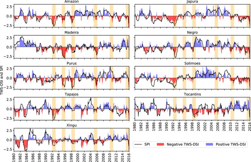
2846                                                      S. Chaudhari et al.: Multi-decadal hydrologic change and variability

                                                                      series (Figs. S3 and S4). However, due to the difficulty in re-
                                                                      solving hillslope processes for low-order streams using 2 km
                                                                      grids, the model is unable to fully capture the flow seasonal-
                                                                      ity in the streams with high topographic gradient.
                                                                         The spatial distribution of the simulated streamflow across
                                                                      the entire model domain and the time series comparison of
                                                                      simulated vs. observed streamflow at 12 selected stations are
                                                                      presented in the Supplement (Figs. S2 and S3). The simu-
                                                                      lated seasonal cycle compares well with the observed one for
                                                                      the entire basin (i.e., Obidos station) as well as for most sub-
                                                                      basins; however, discrepancies in the seasonal peaks can be
                                                                      seen in some basins (e.g., Xingu, Tocantins, and Tapajos).
                                                                      Man-made reservoirs generally attenuate streamflow peaks
                                                                      and seasonal variability, reducing the SD, which is reflected
                                                                      in the observed data but not yet accounted for in the model;
                                                                      this could have exaggerated the SD ratio in some cases. For
                                                                      example, the streamflow in the Tocantins River shows higher
                                                                      SD compared to observed streamflow, likely due to the oper-
                                                                      ation of the Tucurui I and II dams. Conversely, the SD ratio
                                                                      is lower than unity at some stations, including those on the
Figure 1. Taylor diagram showing the correlation and standard de-     Madeira River (Fig. 1), due to the dry bias found in the in-
viation ratio between the simulated and observed streamflow at 55     put precipitation (see Fig. S5 and Sect. 3.2). For sub-basins
gauge stations across the Amazon. The locations of the 55 gauge
                                                                      with higher groundwater contribution to streamflow, such
stations are shown in Fig. S2. Highlighted points with a black bor-
                                                                      as Xingu, Tapajos, Tocantins, and Madeira, the dry-season
der are the gauge stations for which time series comparisons are
shown in Figs. S3 and S4. The size of the markers indicates the an-   flow is overestimated (Fig. S3), which results from possibly
nual mean simulated streamflow at that station, whereas the color     exaggerated groundwater buffer in the model for these re-
indicates the Amazon sub-basin in which the station is located. The   gions (Miguez-Macho and Fan, 2012a). Given that LHF is a
linear distance between each marker and the observed data (i.e.,      continental-scale model, simulates streamflow on a full phys-
OBS; the black dot) is proportional to the root mean square error     ical basis, and is not calibrated with observed streamflow, we
(RMSE).                                                               consider these results to be satisfactory to study the hydro-
                                                                      logic changes and variability.

3     Results and discussion                                          3.2   Evaluation of simulated TWS anomalies with
                                                                            GRACE
3.1    Evaluation of simulated streamflow
                                                                      Figure 2 presents the comparison of simulated TWS anoma-
Figure 1 presents the Taylor diagram (Taylor, 2001) illustrat-        lies and GRACE data for the entire Amazon basin and its
ing the statistics of the simulated streamflow against obser-         eight sub-basins; for model results, the individual TWS com-
vations at 55 gauging locations (see Sect. 2.4.1 and Fig. S2)         ponents are also provided. The model performs very well
across the entire Amazon basin. The Taylor diagram provides           in simulating the basin-averaged TWS anomalies for the
a synthetic view of error in the simulations in terms of the ra-      entire Amazon basin and most sub-basins. However, some
tio of standard deviation (SD) of the simulated streamflow            differences between the simulated and GRACE-based TWS
to the observed as a radial distance and their correlation as         anomaly are evident, especially in sub-basins with a rel-
an angle in the polar axis. Most of the stations show a high          atively smaller area and elongated shape (e.g., Purus and
correlation (> 0.8) and a SD ratio close to unity, indicating         Japura). Note that the accuracy of GRACE–model agreement
a good model performance overall for varying geographi-               is generally low in such small basins due to high bias and
cal locations and stream sizes over the Amazon. Low cor-              leakage correction errors (Chaudhari et al., 2018; Felfelani
relation (∼ 0.6) is seen for some gauging stations situated           et al., 2017; Longuevergne et al., 2010), reflected by higher
on streams with smaller annual mean flow and steep slope              root mean square error (RMSE) values in Fig. 2. Simulated
profile, for example, the smaller streams across the Andes            TWS evidently follows precipitation anomalies (shown in
in Japura and Negro sub-basins, along with the streams in             grey bars in Fig. 2), implying that any uncertainties in the
the northeastern parts of the Amazon. In these streams with           precipitation forcing could have directly impacted TWS. For
high topographic gradients, precipitated water quickly flows          example, the simulated TWS peak in 2002 in the Solimoes
away, causing slightly erratic patterns of seasonal stream-           River basin results from the anomalous high precipitation;
flow, which is apparent in both simulated and observed time           however this could not be validated due to a data gap in

Hydrol. Earth Syst. Sci., 23, 2841–2862, 2019                                       www.hydrol-earth-syst-sci.net/23/2841/2019/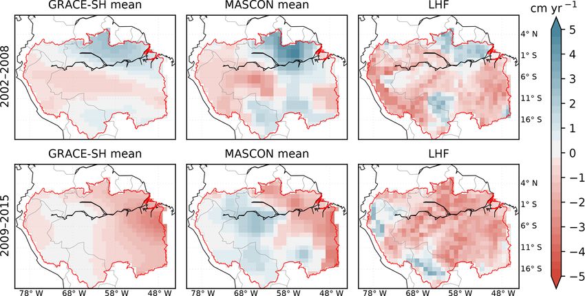
S. Chaudhari et al.: Multi-decadal hydrologic change and variability                                                              2847

Figure 2. Comparison of simulated TWS anomalies from LHF and TWS anomalies obtained from GRACE for the entire Amazon and its
eight sub-basins for the 2002–2015 period. Basin-averaged precipitation anomalies obtained from the WFDEI forcing dataset are also shown
as grey bars. Seasonal cycles of GRACE and simulated TWS are shown in the right panel of each basin along with the simulated individual
TWS components. GRACE results are shown as the mean of the spherical harmonics (SH) solutions from three different processing centers
(i.e., CSR, JPL, and GFZ) and mascon solutions from CSR and JPL. Simulated TWS anomalies are calculated with respect to the GRACE
anomaly window of 2004–2009 for consistency.

GRACE. Overall, the model performance is better in the first          with large floodplains cause floodwater storage to be equally
half of the simulation period (i.e., 2002–2008) compared to           prominent.
the second half, especially in the western sub-basins includ-
ing the Solimoes and Japura, which could be partially at-             3.3   Trends in simulated TWS and comparison with
tributed to the decreasing trend in the precipitation forcing               GRACE
noted in Fig. S6.
   Figure 2 also shows the seasonal cycle including the con-          Here, we present a more detailed examination of the simu-
tribution of different storage components to TWS. In all the          lated TWS by comparing its spatial variability and trend with
basins, the simulated seasonal cycle matches extremely well           GRACE data. Because a shift in agreement between model
with GRACE, adding more confidence to the model results.              and GRACE was detected in Figs. 2 and S7, we conduct a
TWS signal is sturdily modulated by the sub-surface water             trend analysis for two different time windows: 2002–2008
storage, demonstrating the importance of groundwater in the           and 2009–2015 (Fig. 3). It is evident from Fig. 3 that the
Amazon, especially in the southwestern sub-basins. The in-            model captures the general spatial pattern of TWS trend in
verse relationship in the seasonal cycle of two sub-surface           GRACE and its north–south and east–west gradients espe-
water stores, viz. soil moisture and groundwater, is readily          cially for the first half of the analysis period; however, no-
discernable in Fig. 2, which is caused by the competing use           table differences are evident in the second half (2009–2015),
of the sub-surface compartment by the two terms (Felfelani et         particularly over the Madeira River basin. This is a note-
al., 2017; Pokhrel et al., 2013). However, in some sub-basins,        worthy observation given that the basin-averaged TWS vari-
such as the Purus, Solimoes, and Negro, the low-lying areas           ability matches extremely well with GRACE data (Fig. 2)
                                                                      and thus warrants further investigation. There could be a

www.hydrol-earth-syst-sci.net/23/2841/2019/                                         Hydrol. Earth Syst. Sci., 23, 2841–2862, 2019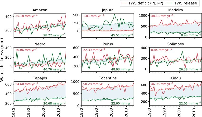
2848 S. Chaudhari et al.: Multi-decadal hydrologic change and variability
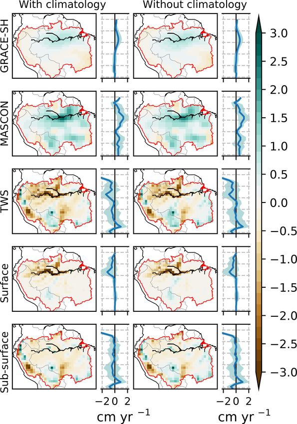
Figure 3. Temporal trend of GRACE solutions compared to the trend in simulated TWS from LHF for the Amazon River basin for two
different time periods. GRACE-SH trends displayed are mean trends computed from water thickness anomalies obtained from CSR, GFZ,
and JPL processing centers, whereas the mascon mean trend is computed from anomalies obtained from CSR and JPL centers.
number of factors contributing to the disagreement, some of by the negative trend observed in the WFDEI precipitation
which could be model-specific (e.g., wet bias in simulated (Fig. S6), concentrated over the Andes region which even-
discharge; Fig. S3); however, this is a general pattern ob- tually drains into the main stem of the Amazon through the
served in many hydrological models as reported in a recent Solimoes River. Due to steep topography, the impact of de-
study (Scanlon et al., 2018). creased precipitation over the Andes range is carried over
Scanlon et al. (2018) indicated a low correlation between to its foothills in terms of runoff, hence corresponding well
GRACE and models, which they attributed to the (i) lack with the negative trends in simulated surface water storage
of surface water and groundwater storage components in over the Central Amazon (Fig. 4). Lower recharge rates in
most of the models, (ii) uncertainty in climate forcing, and the region with decreasing precipitation trend (Fig. S6) are
(iii) poor representation of human intervention in the models also very likely, which is supported by the negative trend vis-
(Scanlon et al., 2018; Sun et al., 2019). Here, we shed more ible in the sub-surface water storage in Fig. 4, over the north-
light on the disagreement issue by investigating the contribu- west region of the Amazon. Hence, it can be concluded that,
tions from the explicitly simulated surface and sub-surface even though the model shows some bias in TWS compared
storage components and their latitudinal patterns, address- to GRACE data, the model accurately represents the key hy-
ing the first concern noted above which is the most criti- drologic processes in the Amazon basin; yet, these results
cal among the three in the Amazon because of the vary- should be interpreted with some caution while acknowledg-
ing contribution of different stores across scales (Pokhrel et ing the uncertainty in the forcing dataset. We also empha-
al., 2013). Figure 4 shows trends in TWS anomalies from size that it is important to evaluate models using spatiotem-
GRACE products and the LHF simulation for the complete poral trends, especially with GRACE, instead of just using
model–GRACE overlap period (i.e., 2002–2015) with clima- the basin-averaged time series, a commonly used approach
tology and with climatology removed; for LHF results, the in most previous studies.
surface and sub-surface component contributions to the TWS
are shown. Also shown in the figure are the zonal means. 3.4 Interannual and interdecadal TWS change and
Simulated TWS from the LHF model displays a higher variability
correlation with GRACE trends compared to most of the
global models discussed in Scanlon et al. (2018). Due to
Figure 5 show the interdecadal shifts in mean simulated TWS
the incorporation of a groundwater scheme and other sur-
(total and its components) for the simulation period. Sev-
face water dynamics, the trend in basin-averaged TWS with
eral observations can be made from this figure. First, the
climatology removed for the Amazon River basin is found
change between the 2010s and 2000s suggests high nega-
to be −1.64 mm yr−1 , much less negative than most of the
tive anomalies in all the water stores, especially over Central
simulated TWS trends reported in Scanlon et al. (2018).
Amazon. This is likely a result of increasing drought occur-
The difference in the sign of trend can partly be explained
rence and severity in the region, e.g., the 2010 (Lewis et al.,
Hydrol. Earth Syst. Sci., 23, 2841–2862, 2019 www.hydrol-earth-syst-sci.net/23/2841/2019/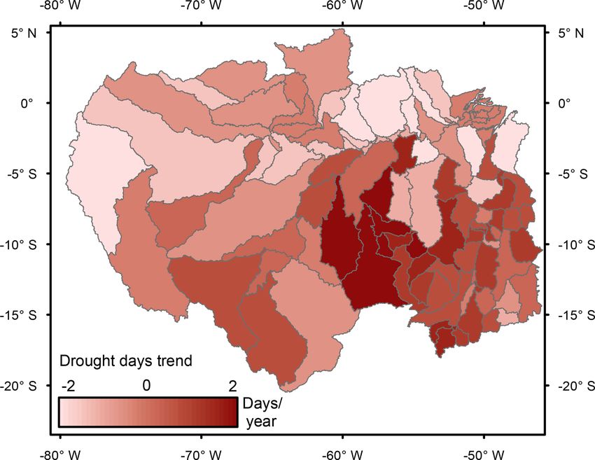
S. Chaudhari et al.: Multi-decadal hydrologic change and variability 2849
(Fig. S6), the regional hydrologic changes in terms of TWS
are also prominent. Another peculiar phenomenon observed
at the decadal scale is the start of the negative anomaly in
groundwater storage over the Central Amazon. A small but
spatially well distributed below-decadal-average water table
(dictated by groundwater storage) is evident in the Central
Amazon region and the upper stretches of the Madeira basin
during the 2010s (Fig. 5, column 3, row 4). Since the water
table is shallow, and groundwater is the major contributor of
streamflow in this region (Miguez-Macho and Fan, 2012a),
some part of the negative anomaly in surface water stores
can be attributed to the below-decadal-average groundwater
table.
Significant long-term trends in simulated TWS and its
components are evident in sizeable portions of the basin
(Fig. 6). While a negative trend is found in the southern and
southeastern regions (e.g., Madeira, Tapajos, Xingu and To-
cantins), the trend is positive in the northern and western re-
gions (Solimoes and Negro) (see Fig. S9 for basin-averaged
trends). Being the major contributor, sub-surface water stor-
age mimics the trend patterns in TWS (see Sect. 3.2). On the
contrary, surface water storage trends are mainly dominated
by floodwater and are concentrated along the main stem of
the Amazon and the upper reaches of the Negro. The positive
trends in floodwater can be explained by the corresponding
trends in input precipitation (Fig. S5). Excess precipitation in
sub-basins, such as the Solimoes and Negro, which are char-
acterized by a high topographic gradient, is directly trans-
lated in the surface water storage, in this case floodwater.
Figure 4. Same as in Fig. 3 but for the complete model–GRACE Although a corresponding increment in river water storage
overlap period (i.e., 2002–2015). The latitudinal mean is shown on is also expected, its smaller storage makes the trend magni-
the right side of each panel. tudes negligible. Nominal negative trends, but significant, in
floodwater storage are found in the upper reaches of Madeira
as well, corresponding to the negative trends in input precip-
2011; Marengo et al., 2011) and 2015 (Jiménez-Muñoz et al., itation over that region.
2016) Amazonian droughts. Second, although the 2000s en- To provide an in-depth understanding of the interdecadal
compassed one of the severe Amazonian droughts, viz. 2005 changes occurring in the Amazon region and to determine
(Marengo et al., 2008; Zeng et al., 2008), its impact was whether the changes observed in Fig. 5 are significant, we
not pronounced in terms of the decadal mean, which could applied a t test methodology to the long-term TWS anoma-
be due to the offset caused by anomalous wet years includ- lies at basin and sub-basin levels. The spatial changes ob-
ing 2006 and 2009 (Chen et al., 2010; Filizola et al., 2014). served in Fig. 5 are summarized with their interdecadal sig-
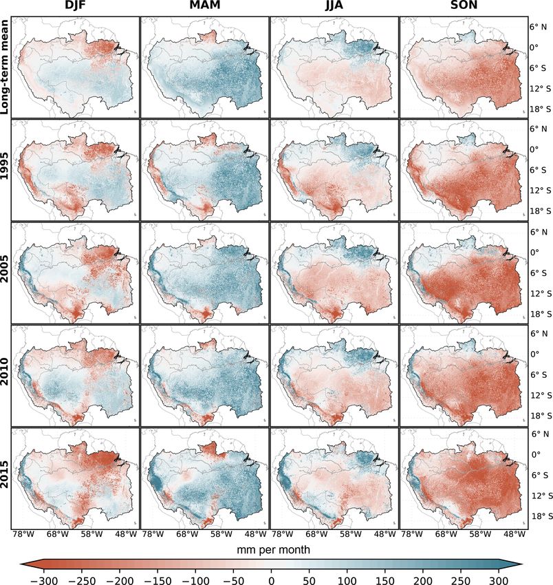
Third, we find an increase in river water storage in the north- nificance in Table S1 (Supplement), along with the decadal
western region and decrease in the southwest of the Amazon means and standard deviations. Significant change at 99 %
on a decadal scale (Fig. 5, column 1, row 2), which is in line level is found in the Negro River basin throughout the study
with the findings reported in previous studies based on the period, followed by the Solimoes River basin exhibiting sig-
observed streamflow in 18 sub-basins for the 1974–2004 pe- nificant change in the last three decades. These changes can
riod (Espinoza et al., 2009; Wongchuig Correa et al., 2017). be attributed to the corresponding changes in precipitation
The most remarkable feature we observe in Fig. 5 is the (Fig. S5), which follow a similar change in respective basins.
exceptional interdecadal shifts between the 2000s and 2010s. However, the significant hydrologic changes in the Tocantins
The central and northwestern part of the Amazon region, en- and Madeira can be primarily attributed to LULC changes,
compassing the Negro and Solimoes, along with some parts as the corresponding changes in precipitation were relatively
of the Madeira in the southwest, experienced a major decadal negligible. For example, the Tocantins River basin under-
dry spell compared to the previous decades. Although a ma- went major LULC changes in response to heavy deforesta-
jor part of this decadal dry condition could be attributed to the tion caused by dam construction and cattle farming (Costa et
decreasing trend in input precipitation discussed in Sect. 3.3 al., 2003) until policies were imposed in 2004 by the Brazil-
www.hydrol-earth-syst-sci.net/23/2841/2019/ Hydrol. Earth Syst. Sci., 23, 2841–2862, 2019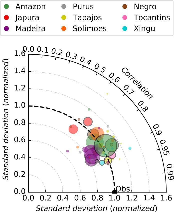
2850                                                     S. Chaudhari et al.: Multi-decadal hydrologic change and variability

Figure 5. Interdecadal difference between individual water store and TWS storage for the period of 1980–2015 at the original ∼ 2 km model
grids. The changes are displayed as the difference between consecutive decadal means for TWS and its components. Decadal windows are
1980–1989 as 1980s, 1990–1999 as 1990s, 2000–2009 as 2000s, and 2010–2015 as 2010s. Note that the 2010s period consists of only six
years, and the ranges of color bars differ among the plots.

Hydrol. Earth Syst. Sci., 23, 2841–2862, 2019                                        www.hydrol-earth-syst-sci.net/23/2841/2019/
S. Chaudhari et al.: Multi-decadal hydrologic change and variability                                                                     2851

Figure 6. Temporal trend in simulated TWS and its components (i.e., sub-surface water, floodwater, and river water stores) for the period of
1980 to 2015 expressed in centimeters per year (cm yr−1 ). Markers indicate significant trends at the 99 % level. Note that the ranges of color
bars differ among the plots.

ian government (captured in the ESA dataset; Fig. S8). Sim-               a similar magnitude and spatial impact on the sub-surface
ilarly, the Madeira River basin also endured major LULC                   storage; however, the 2005 drought was more intense and
changes in the late 1990s, which were dominated by agri-                  dramatic in the Solimoes River basin, findings also noted in
cultural expansion (Dórea and Barbosa, 2007).                             previous studies (Marengo et al., 2008; Phillips et al., 2009;
                                                                          Zeng et al., 2008). Similarly, the more recent drought in 2015
3.5     Interannual and interdecadal drought evolution                    had a more pronounced impact in the eastern and northeast-
                                                                          ern region and average impact on the other parts of the basin.
3.5.1    Severity of TWS drought                                          Due to the shallow water table in the Amazonian lowlands,
                                                                          sub-surface storage acts as a buffer during the low precipi-
In this section, we examine the time evolution of droughts                tation events, hence facing higher anomalies during drought
and quantify their impacts on TWS variability by using                    conditions compared to the long-term mean. As the Negro
TWS-DSI. The use of TWS-DSI enables the depiction of                      River (i.e. northern region of the Amazon) basin experiences
a “bigger picture” encompassing all water stores that rep-                an opposite seasonal phase compared to the rest of the Ama-
resent the vertically integrated total water availability dur-            zon region, the drought conditions in this basin are observed
ing droughts and dictate the streamflow. Figure 7 shows the               during the period of December to March. The opposite sea-
TWS-DSI for individual Amazonian sub-basins and the 12-                   sonal cycle of precipitation and flooding in the north and
month Standardized Precipitation Index (SPI) (Mckee et al.,               south banks of the Amazon mitigates the number of floods
1993) calculated from the basin-averaged precipitation time               and droughts in the basin as a whole while resulting in more
series. As expected TWS-DSI follows a similar pattern of the              dramatic floods or droughts in particular sub-basins (e.g., To-
SPI, but differences in the index peaks can be noted for the              cantins, Tapajos and Madeira).
drought years. For example, the 2005 drought was prominent
in terms of TWS in the southwest region, comprising Pu-                   3.5.2   Time evolution of dry-season total deficit and
rus and Madeira rivers, with TWS-DSI going as high as −3,                         TWS release
whereas the corresponding SPI values were −1.78 and −2.2,
respectively. Similarly, severe TWS drought (e.g., 2001) is               The dry-season TWS variability is examined by using the
detected in the southeastern basins of the Amazon (Madeira,               cumulative difference between PET and P , termed as the
Xingu, and Tocantins); however, the corresponding SPI val-                TWD (see Sect. 2.7). Further, to examine the response from
ues are negligible. The sub-surface storage (major contribu-              TWS against TWD, we quantify the TWS-R, hence creat-
tor of TWS in these sub-basins) characteristic can be noted               ing a supply–demand relationship between them. Figure S10
in these cases which has a delayed response from the preced-              shows TWD, the corresponding TWS-R, and the total contri-
ing series of low precipitation events due to a slow residence            bution of the surface water storage to TWS-R for the extreme
time.                                                                     drought years during 1980–2015 compared to their respec-
   The impact of drought conditions on TWS is quantified                  tive long-term means. Spatial patterns in TWD and TWS-
by examining the seasonal dynamics in the simulated sub-                  R are analogous to the patterns in the simulated sub-surface
surface water storage for the four most extreme historical                storage during the months of September to November (SON)
drought years during the simulation period (Fig. 8). Although             as seen in Fig. 8. We find that TWS-R receives a fairly equal
no clear trend can be seen in terms of the evolution of the               contribution from surface (along the rivers) and sub-surface
drought impact on sub-surface water storage, the spatial vari-            (soil moisture and groundwater) water stores (rest of the re-
ability between different drought years is readily discernible.           gion); however, the latter is more dominant during drought
For example, the 1995 and 2010 droughts more or less had                  years. A clear positive trend in drought years is visible in

www.hydrol-earth-syst-sci.net/23/2841/2019/                                             Hydrol. Earth Syst. Sci., 23, 2841–2862, 2019
2852 S. Chaudhari et al.: Multi-decadal hydrologic change and variability
Figure 7. TWS drought severity index (TWS-DSI) calculated using the simulated TWS from LHF for Amazon and its sub-basins. TWS-DSI
is calculated using basin-averaged TWS anomalies on a monthly scale. Shaded areas indicate the severe drought years reported in the past
literature. The black line is the 12-month Standardized Precipitation Index (SPI) calculated by using basin-averaged precipitation data from
the WFDEI forcing dataset.
Fig. S10, indicating an increase in TWS-R, with a signifi- as deforestation activities, generally increase streamflow and
cant sub-surface contribution, especially in the southeastern are also known to offset the impact on streamflow caused by
part of the Amazon. This change can be directly attributed a decrease in precipitation over the Amazon (Panday et al.,
to the major LULC changes occurring in the basin, caus- 2015), this mechanism is dominant mostly during the wet
ing loss of TWS to evapotranspiration through agricultural season. In the dry season, however, the streams in the Ama-
expansion, especially in the Tocantins, Xingu, Tapajos, and zon are fed primarily by the sub-surface water storage (see
Madeira river basins (Chen et al., 2015; Costa et al., 2003; Sect. 3.2), which is negatively impacted by deforestation ac-
Dórea and Barbosa, 2007). tivities (e.g., increased regional evapotranspiration).
3.5.3 Hydrological drought trends in Amazonian 3.6 Comprehensive characterization of Amazonian
sub-catchments droughts
The hydrological drought behavior of each sub-basin is char- As a first attempt to comprehensively characterize the Ama-
acterized by quantifying the drought days per year at the zonian droughts, we present a summary of all the drought
Level-5 HydroBASINS scale (Lehner and Grill, 2013), re- characteristics discussed in the previous sections on a spi-
ferred here to as “sub-catchments”. Based on the stream- der plot (Fig. 10). Each spider plot is a representation of a
flow simulated at the most downstream grid in the sub- drought year with respect to the (i) causes of drought and
catchments, temporal trends for the 1980–2015 period are their type in terms of common indices; (ii) response of differ-
calculated and presented in Fig. 9. Significant trends in ent water stores, such as TWS, to the drought event; (iii) role
drought durations are discernible in the Tapajos and Madeira of groundwater storage in alleviating the dry conditions on
sub-basin along with the southeastern portions of the Ama- the surface; and (iv) the spatial impact of the drought in
zon, congruent with the heavy deforestation activities found different sub-basins of the Amazon. Although no signifi-
in these sub-basins (Chen et al., 2015; Costa et al., 2003; cant trend in the combined drought characteristic is appar-
Dórea and Barbosa, 2007). Although LULC changes, such ent, Fig. 10 provides important insights into the variability
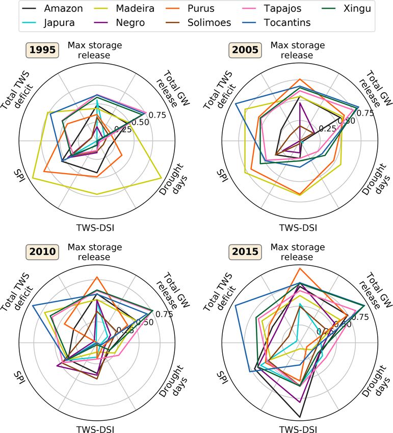
Hydrol. Earth Syst. Sci., 23, 2841–2862, 2019 www.hydrol-earth-syst-sci.net/23/2841/2019/S. Chaudhari et al.: Multi-decadal hydrologic change and variability 2853 Figure 8. Seasonal dynamics of simulated sub-surface water storage from LHF in the Amazon River basin for extreme droughts during the simulation period. Long term mean is the mean seasonal anomaly for the 1980–2015 period, where DJF is December to February, MAM is March to May, JJA is June to August, and SON is September to November. of Amazonian droughts. It is evident from the figure that the water exchange is the key mechanism behind this unique drought variability over the years was significant in terms of behavior, causing groundwater to fulfill the drought deficit both magnitude and spatial impact. The most notable fea- in streamflow over the basin. Due to shallow water tables ture in Fig. 10 is the distinct relationship between the SPI at the downstream end of these basins, a significant quan- and drought duration. For example, during the 1995 drought, tity of groundwater is fed to the rivers, which manifests as most of the river basins (e.g., Tocantins, Tapajos, Xingu, high peaks in total groundwater release, evident in Fig. 10. and Negro) experienced significant meteorological and TWS Similarly, a high number of drought days are found cor- droughts; however, the severity of hydrological droughts was responding to less groundwater release, such as during the relatively negligible in those basins. Groundwater–surface 1995 drought in Madeira. Conversely, TWS-DSI generally www.hydrol-earth-syst-sci.net/23/2841/2019/ Hydrol. Earth Syst. Sci., 23, 2841–2862, 2019
2854                                                     S. Chaudhari et al.: Multi-decadal hydrologic change and variability

Figure 9. Trends in drought duration per year in the Amazon at a
Level-5 HydroBASINS scale as defined in Lehner and Grill, (2013),
derived by using the Q90 threshold from the simulated streamflow
by the LHF model. Darker colors indicate the higher positive trend
magnitudes.

follows the same pattern as that of the SPI but with a lesser        Figure 10. Intercomparison and comprehensive characterization of
                                                                     the severe drought events during the study period in the Amazon
magnitude, which can be attributed to the delayed response
                                                                     River basin and its sub-basins. Color coding in each subplot rep-
from groundwater.
                                                                     resents individual river basins. Note that all variables are basin av-
   Further, the behavior of the Amazonian sub-basins can be          erages normalized (0–1) for each variable over all drought years.
characterized by the shape of the polygon formed by the              The bottom half of the variables in the figure are drought in-
comparison of different aspects of past droughts. The con-           dices representing different types of droughts: TWS-DSI denotes
vex and concave characteristic in the plots mainly depends           TWS drought severity index (Sect. 2.7), SPI (Standardized Pre-
on the interrelation between meteorological and hydrologi-           cipitation Index) represents meteorological drought severity, and
cal drought indices, which is further controlled by the sub-         “drought days” represents hydrological drought severity in the basin
surface water storage. A convex polygon indicates a lower            (Sect. 2.6). The top half of the variables quantify the water deficit in
groundwater contribution to streamflow in the sub-basin,             terms of total TWS deficit (cumulative PET-P), water supply as the
such as in Purus during 1995 and 2005, whereas a concave             TWS release (max storage release), and the groundwater contribu-
                                                                     tion of TWS release (total GW release).
polygon suggests higher groundwater release to streamflow
in that particular year.

3.7    Intensification of the Amazonian dry season                   torical drought events in earlier sections. We note that the
                                                                     trends in the total deficit should be interpreted with caution
Results suggest an increasing trend in TWD with significant          as the uncertainty in the forcing could have affected TWD
decadal variability over the Amazon and its sub-basins, indi-        and TWS-R trend estimates.
cating an increase in dry-season length over the past 36 years          We find that the river basins that contain high altitudi-
(Fig. 11). Further, the increasing gap between TWD and               nal areas (Purus, Solimoes, and Negro) have a fairly bal-
TWS-R suggests an intensified terrestrial hydrologic sys-            anced relationship between TWD and TWS-R, but southern
tem over the dry season during the study period. As the              and southeastern sub-basins exhibit a higher water deficiency
LULC impact is partly accounted for in the PET calcula-              (Fig. S11), with approximately 2- to 3-fold differences be-
tions (i.e., through changing surface albedo), the river basins      tween TWD and TWS-R during regular years. For drought
with substantial LULC change, such as Madeira, Tapajos,              years, however, the difference between TWD and TWS-R is
Tocantins, and Xingu, portray higher TWD trend magnitudes            even higher, creating highly anomalous dry conditions in the
(significance > 95 %). The peaks in the TWD correspond               sub-basins. Consistent higher values of TWD in southern and
well with drought years; for example, the peaks in the TWD           southeastern sub-basins of the Amazon further highlight the
for Madeira are analogous to the drought years (e.g., 1988,          intensification of the dry season, with increasing water de-
1995, 2005, and 2010). Due to this definitive response to            ficiency corresponding to an almost constant water supply
drought conditions, TWD is also used to characterize his-            from TWS-R. This phenomenon is also highlighted in Es-

Hydrol. Earth Syst. Sci., 23, 2841–2862, 2019                                       www.hydrol-earth-syst-sci.net/23/2841/2019/
You can also read