Real-time UV index retrieval in Europe using Earth observation-based techniques: system description and quality assessment
←
→
Page content transcription
If your browser does not render page correctly, please read the page content below
Atmos. Meas. Tech., 14, 5657–5699, 2021
https://doi.org/10.5194/amt-14-5657-2021
© Author(s) 2021. This work is distributed under
the Creative Commons Attribution 4.0 License.

Real-time UV index retrieval in Europe using Earth
observation-based techniques: system description
and quality assessment
Panagiotis G. Kosmopoulos1 , Stelios Kazadzis2 , Alois W. Schmalwieser3 , Panagiotis I. Raptis1 ,
Kyriakoula Papachristopoulou4 , Ilias Fountoulakis4,5 , Akriti Masoom6 , Alkiviadis F. Bais7 , Julia Bilbao8 ,
Mario Blumthaler9 , Axel Kreuter9,10 , Anna Maria Siani11 , Kostas Eleftheratos12 , Chrysanthi Topaloglou7 ,
Julian Gröbner2 , Bjørn Johnsen13 , Tove M. Svendby14 , Jose Manuel Vilaplana15 , Lionel Doppler16 , Ann R. Webb17 ,
Marina Khazova18 , Hugo De Backer19 , Anu Heikkilä20 , Kaisa Lakkala21 , Janusz Jaroslawski22 , Charikleia Meleti7 ,
Henri Diémoz5 , Gregor Hülsen2 , Barbara Klotz9 , John Rimmer17 , and Charalampos Kontoes4
1 Institute for Environmental Research and Sustainable Development,
National Observatory of Athens (IERSD/NOA), Athens, Greece
2 Physikalisch-Meteorologisches Observatorium Davos, World Radiation Center (PMOD/WRC), Davos Dorf, Switzerland
3 Unit of Physiology and Biophysics, University of Veterinary Medicine, Vienna, Austria
4 Institute for Astronomy, Astrophysics, Space Applications and Remote Sensing,

National Observatory of Athens (IAASARS/NOA), Athens, Greece
5 Regional Environmental Protection Agency (ARPA) of the Aosta Valley, Saint-Christophe, Italy
6 Mechanical and Industrial Engineering Department, Indian Institute of Technology, Roorkee, India
7 Laboratory of Atmospheric Physics, Aristotle University of Thessaloniki, Thessaloniki, Greece
8 Atmosphere and Energy Laboratory, Valladolid University, Valladolid, Spain
9 Division for Biomedical Physics, Innsbruck Medical University, Innsbruck, Austria
10 LuftBlick, Earth Observation Technologies, Mutters, Austria
11 Physics Department, Sapienza University of Rome, Rome, Italy
12 Faculty of Geology and Geoenvironment, National and Kapodistrian University of Athens, Athens, Greece
13 Section for Non-Ionizing Radiation, Norwegian Radiation and Nuclear Safety Authority, Bærum, Norway
14 Department of Atmospheric and Climate Research, NILU – Norwegian Institute for Air Research, Kjeller, Norway
15 Department of Atmospheric Research and Instrumentation, National Institute for Aerospace Technology,

Torrejón de Ardoz, Spain
16 Deutscher Wetterdienst, Meteorologisches Observatorium Lindenberg – Richard Assmann Observatorium

(DWD, MOL-RAO), Lindenberg, Germany
17 Department of Earth and Environmental Sciences, University of Manchester, Manchester, UK
18 Centre for Radiation, Chemical and Environmental Hazards, Public Health England, London, UK
19 Observations Department, Royal Meteorological Institute of Belgium, Brussels, Belgium
20 Climate Research Programme, Finnish Meteorological Institute, Helsinki, Finland
21 Space and Earth Observation Centre, Finnish Meteorological Institute, Sodankylä, Finland
22 Department of Atmospheric Physics, Institute of Geophysics, Polish Academy of Sciences, Warsaw, Poland

Correspondence: Panagiotis G. Kosmopoulos (pkosmo@noa.gr)

Received: 21 December 2020 – Discussion started: 1 March 2021
Revised: 17 July 2021 – Accepted: 26 July 2021 – Published: 19 August 2021

Published by Copernicus Publications on behalf of the European Geosciences Union.
5658                                     P. G. Kosmopoulos et al.: The UVIOS system: description and quality assessment

Abstract. This study introduces an Earth observation (EO)-        is linked to a number of medical implications (Lucas et al.,
based system which is capable of operationally estimating         2015).
and continuously monitoring the ultraviolet index (UVI) in           The UV index was introduced by the WHO/WMO in 1994
Europe. UVIOS (i.e., UV-Index Operating System) exploits          (WMO, 1995) as a simple method of informing the general
a synergy of radiative transfer models with high-performance      public about the erythema effective (sun-burning) UV. It is
computing and EO data from satellites (Meteosat Second            a unitless, scaled version of erythemally weighted UV de-
Generation and Meteorological Operational Satellite-B) and        termined by multiplying the erythema weighted irradiance
retrieval processes (Tropospheric Emission Monitoring Inter-      (in W m−2 ) by 40 m2 W−1 (Fioletov et al., 2010; Vanicek et
net Service, Copernicus Atmosphere Monitoring Service and         al., 2000; WHO, 2002). The response of UV radiation to cli-
the Global Land Service). It provides a near-real-time now-       matic changes is of great concern (Bais et al., 2019, 2018;
casting and short-term forecasting service for UV radiation       McKenzie et al., 2011). According to the latest work of Bais
over Europe. The main atmospheric inputs for the UVI simu-        et al. (2019), greater values of UV are expected by the end
lations include ozone, clouds and aerosols, while the impacts     of the 21st century, relative to the present decade, at low lat-
of ground elevation and surface albedo are also taken into ac-    itudes, while at higher latitudes UV will decrease, but these
count. The UVIOS output is the UVI at high spatial and tem-       projections are associated with high uncertainty (up to 30 %).
poral resolution (5 km and 15 min, respectively) for Europe          There are many factors affecting UV irradiance reaching
(i.e., 1.5 million pixels) in real time. The UVI is empirically   Earth’s surface (Kerr and Fioletov, 2008). The dependence of
related to biologically important UV dose rates, and the relia-   UV irradiance on astronomical and geometrical parameters is
bility of this EO-based solution was verified against ground-     generally well understood, and in many cases the changes are
based measurements from 17 stations across Europe. Sta-           periodical (e.g., Blumthaler et al., 1997; Gröbner et al., 2017;
tions are equipped with spectral, broadband or multi-filter in-   Larkin et al., 2000; Seckmeyer et al., 2008). Atmospheric
struments and cover a range of topographic and atmospheric        gases play a crucial role in attenuating UV irradiance; specif-
conditions. A period of over 1 year of forecasted 15 min          ically, NO2 is a major absorber in the UV (e.g., Cede et al.,
retrievals under all-sky conditions was compared with the         2006), while O3 is the main absorber at lower (UVB) wave-
ground-based measurements. UVIOS forecasts were within            lengths. Other gases that have significant absorption in the
±0.5 of the measured UVI for at least 70 % of the data com-       UV include SO2 (Fioletov et al., 1998) and HCHO (Gratien
pared at all stations. For clear-sky conditions the agreement     et al., 2007), but their – usually – smaller atmospheric abun-
was better than 0.5 UVI for 80 % of the data. A sensitivity       dances result in minor effects on incoming UV (with major
analysis of EO inputs and UVIOS outputs was performed in          exceptions such as volcanic incidents). Aerosols are another
order to quantify the level of uncertainty in the derived prod-   important parameter controlling UV irradiance levels at the
ucts and to identify the covariance between the accuracy of       surface (e.g., Kazadzis et al., 2009b). Aerosol optical depth
the output and the spatial and temporal resolution and the        (AOD) that quantifies the attenuation of the direct solar beam
quality of the inputs. Overall, UVIOS slightly overestimated      by aerosols is a parameter varying with wavelength. Single
the UVI due to observational uncertainties in inputs of cloud     scattering albedo (SSA), which determines the scattering ra-
and aerosol. This service will hopefully contribute to EO ca-     tio to total extinction, is also a spectrally variant parameter.
pabilities and will assist the provision of operational early     Several recent studies based on surface UV irradiance mea-
warning systems that will help raise awareness among Euro-        surements or calculations reveal the enhanced absorption by
pean Union citizens of the health implications of high UVI        aerosols in the UV relative to the visible spectral range. Fi-
doses.                                                            nally, a number of studies have highlighted the importance of
                                                                  using representative SSA in the UV spectral region instead
                                                                  of interpolating SSA at visible wavelengths to the UV or di-
                                                                  rectly using SSA at visible wavelengths, options that system-
1   Introduction                                                  atically overestimate UV irradiance (Corr et al., 2009; Foun-
                                                                  toulakis et al., 2019; Kazadzis et al., 2016; Mok et al., 2018;
Human exposure to ultraviolet (UV) radiation (< 400 nm)           Raptis et al., 2018).
has both beneficial and harmful effects (Andrady et al., 2015;       All the aforementioned parameters are particularly impor-
Juzeniene et al., 2011; Lucas et al., 2006). Overexposure to      tant under cloud-free conditions. The cloudy sky compli-
UV radiation (UVR) has a number of implications, such as          cates the propagation of solar radiation, predominantly in the
the acute response of erythema, the risk of skin cancer and       troposphere, through multiple cloud–radiation interactions.
a number of eye diseases (snow blindness, cataract). Nev-         Nonetheless, UVR is less affected than the total solar radia-
ertheless, exposure to solar UVB radiation (290–315 nm) is        tion by clouds (e.g., Badosa et al., 2014). Bais et al. (1993)
the main mechanism for the synthesis of vitamin D in hu-          quantified that for the city of Thessaloniki the change from 0
man skin (Holick, 2002; Webb and Engelsen, 2008; Webb et          to 8 oktas for cloud coverage corresponds to 80 % reduction
al., 2011). Low levels of vitamin D are associated with de-       in the UVR and pointed out that there is very low wavelength
pression of the immune system, and there is evidence that it      dependence of UVR attenuation by cloud cover. Although

Atmos. Meas. Tech., 14, 5657–5699, 2021                                            https://doi.org/10.5194/amt-14-5657-2021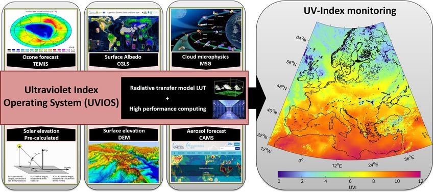
P. G. Kosmopoulos et al.: The UVIOS system: description and quality assessment                                              5659

the transmittance of clouds does not vary significantly with        Europe (Schmalwieser et al., 2017), with all monitoring in-
wavelength, some studies (Mayer et al., 1998; Seckmeyer             struments having the potential to provide other effective
et al., 1996) have found that the diffuse component of the          doses such as the effective dose for the production of vita-
surface UVR is affected by clouds in a spectrally dependent         min D in human skin (e.g., Fioletov et al., 2009).
way due to more efficient scattering and absorption of shorter         There are three types of instruments for UV irradiance
UV wavelengths in the case of large air masses. In cases of         measurements: those measuring the integral of UV irradiance
partially cloudy sky but unobscured Sun, UVR tends to be            (broadband sensors) tailored to a specific response, narrow-
higher than in clear-sky conditions (e.g., Badosa et al., 2014),    band instruments such as filter radiometers with coarse spec-
as is the case for total solar radiation. For short timescale       tral resolution, and instruments performing high-resolution
analysis the variability of UVR introduced by clouds should         spectral measurements – the most versatile but most chal-
be considered.                                                      lenging and least robust instruments. Concerning the cur-
   Solar UV irradiance at the surface increases with increas-       rent UV monitoring measurement accuracy, the European
ing surface albedo. This increment affects the UV radiant ex-       reference UV spectroradiometer (QASUME) is a travel-
posure, which becomes crucial for outdoor human activities          ing instrument which provides a common standard through
(Schmalwieser and Siani, 2018; Schmalwieser, 2020; Siani            inter-comparison on-site (Gröbner et al., 2005; Hülsen et
et al., 2008). Measurements and computations of effective           al., 2016). During the period 2000–2005 QASUME visited
surface albedo for heterogeneous surfaces reveal its strong         27 spectroradiometer sites. Out of the 27 instruments, 13
spectral dependence, with snow-covered surfaces having sig-         showed deviations of less than 4 % relative to the QASUME
nificantly higher values of albedo for short wavelengths com-       reference spectroradiometer in the UVB (for 15 instruments
pared to total solar radiation (Blumthaler and Ambach, 1988;        in the UVA) for solar zenith angles below 75◦ . The expanded
Kreuter et al., 2014). Stronger enhancement of the UV rela-         relative uncertainty (coverage factor k = 2) of solar UV ir-
tive to visible radiation over highly reflective surfaces is also   radiance measurements by QASUME, for solar zenith angle
due to the more effective multiple scattering of shorter wave-      (SZA) smaller than 75◦ and wavelengths longer than 310 nm,
lengths in the atmosphere.                                          was 4.6 % in 2002–2014 (Gröbner and Sperfeld, 2005) and
   Any systematic changes in any of the parameters described        has been 2 % since 2014 (Hülsen et al., 2016). For broadband
in previous paragraphs have the potential to lead to changes        instruments, the current instrument uncertainties are summa-
for UVR. These changes vary significantly throughout the            rized in Hülsen et al. (2020, 2008). In 2017, 75 broadband
globe and are attributed to different possible drivers (Bern-       instruments measuring the UV index and the UVB or/and
hard and Stierle, 2020; Fountoulakis et al., 2018; McKenzie         the UVA irradiance participated in the solar UV broadband
et al., 2019). Fountoulakis et al. (2020a) give a review of re-     radiometer comparison in Davos, Switzerland. Using the in-
cent publications concerning UV trends since the 1990s and          strument/user calibration factors, the differences between the
associated factors, summarizing these as positive trends for        data sets by the broadband instruments and the reference
southern and central Europe and negative trends at higher           (QASUME) data set were within ±5 % for 32 (43 %) of
latitudes and recognizing the important role of aerosols and        the instrument data sets, ±10 % for 48 (64 %) and exceeded
cloud coverage for these trends. Chubarova et al. (2020)            ±10 % for 27 (35 %).
found a long-term increase of 3 % per decade in UV in north-           Although ground-based monitoring of solar UVR is more
ern Eurasia for the 1979–2015 period. For the northern mid-         accurate than satellite retrievals, ground-based stations are
latitudes Zerefos et al. (2012) showed that the long-term           sparse, and the only way for continuous monitoring of the
(1995–2006) positive trend in total ozone was not enough            UVR on a global scale is through satellites. In recent decades
to compensate for, let alone reverse, the UVB increase at-          instruments onboard satellites have provided the necessary
tributed to tropospheric aerosol decline (brightening effect).      data for estimates of UV irradiance reaching the Earth’s sur-
Since 2007, a slowdown or even a possible turning point             face on a global scale (Herman, 2010), and hence satellite-
in the positive UVB trend has been detected, which has              derived UVR climatological studies have been conducted
been attributed to the continued upward trend in total ozone        (Vitt et al., 2020; Verdebout, 2000). The satellite UV irradi-
overwhelming the aerosol effect (Zerefos et al., 2012). By          ance record started with the Total Ozone Mapping Spectrom-
contrast, the long-term variability of UVB irradiance over          eter (TOMS) onboard Nimbus-7 in 1978 and continued with
northern high latitudes was determined by ozone and not by          the Ozone Monitoring Instrument (OMI) onboard NASA’s
aerosol trends, as shown by Eleftheratos et al. (2015), who         satellite EOS-Aura. The OMI retrieval algorithm for surface
found a statistically significant negative trend of −3.9 % per      UVR estimates was based on the experience gained from
decade for the UVB irradiance during the time period 1999–          TOMS (Levelt et al., 2018, 2006). The early surface UVR
2011, in agreement with a statistically significant increase in     retrieval algorithms from satellite data did not account for
spaceborne-measured total ozone by about 1.5 % per decade           the enhanced aerosol absorption in the UV spectral range, re-
(ozone recovery) for the same area.                                 sulting in overestimated values (Krotkov et al., 1998). A lot
   The continuous monitoring of the UV index is currently           of scientific effort has been put into correcting the products
performed by about 160 stations from 25 countries around            (Arola et al., 2009). The TROPOspheric Monitoring Instru-

https://doi.org/10.5194/amt-14-5657-2021                                             Atmos. Meas. Tech., 14, 5657–5699, 2021
5660                                     P. G. Kosmopoulos et al.: The UVIOS system: description and quality assessment

ment (TROPOMI) onboard Sentinel-5 Precursor (Lindfors et           2     UVIOS
al., 2018) is the current satellite instrument that provides the
surface UVR product on a daily basis with global coverage,         2.1    System description
including 36 UVR parameters. As the aforementioned instru-
ments were installed onboard polar-orbiting satellites, pro-       UVIOS is a novel model that uses real-time and forecasted
viding global spatial coverage, the temporal resolution of the     atmospheric inputs based on satellite retrievals and model-
data is daily since there are only one or two overpasses per       ing techniques and databases in order to nowcast and fore-
day for every point. Geostationary satellites provide continu-     cast the UVI with a spatial resolution of 5 km and a tem-
ous (in time) measurements over wide areas. The geostation-        poral resolution of 15 min. The UVIOS calculation scheme
ary meteorological satellites Meteosat monitor the full Earth      is based on the libRadtran library of radiative transfer mod-
disk including Europe, and their frequent data acquisition of      els (RTMs) (Mayer and Kylling, 2005) within which all the
rapidly changing parameters, e.g., cloud, is essential for esti-   available inputs (i.e., solar elevation, cloud and aerosol opti-
mating daily UV doses (Verdebout, 2000).                           cal properties, ozone) can be integrated in real time into the
   Comparison of OMI surface UV irradiance estimates               radiative transfer code and calculate the UVI for each pixel.
with ground-based measurements for Thessaloniki, Greece,           Afterwards, post-processing correction for the elevation of
showed that OMI irradiances overestimate surface observa-          each location and the surface albedo is also performed. In
tions for UVB wavelengths by between ∼ 1.5 % and 13.5 %,           order to be able to simulate the UVI for 1.5 million pixels
in contrast to underestimated satellite values for UVA wave-       in real time, we use pre-determined spectral solar irradiance
lengths (Zempila et al., 2016). Results from the validation        LUTs based on the Libradtran RTM in combination with
of the TROPOMI surface UV radiation product showed                 high-performance computing (HPC) architectures that speed
that most of the satellite data agreed within ±10 % with           up the process of choosing and interpolating/extrapolating
ground-based measurements for snow-free surfaces (Lakkala          the right combinations from the LUTs (Kosmopoulos et al.,
et al., 2020). Larger differences between satellite data and       2018; Taylor et al., 2016). The result is the retrieval of the
ground-based measurements were observed for sites with             UVI for 1.5 million pixels covering the European domain in
non-homogeneous topography and non-homogeneous sur-                less than 5 min after receiving all necessary input parameters.
face albedo conditions. The differences between ground-               As mentioned, the UVIOS architecture does not include
based and satellite UVR data are mostly due to uncertain-          a clear-sky model and the subsequent calculation of individ-
ties in the input parameters to the satellite algorithm used       ual sources of UV attenuation, but instead it directly uses the
to retrieve the UV irradiance at the surface. Based on a re-       following parameters: SZA, AOD and other aerosol optical
cent study of Garane et al. (2019), a mean bias of 0 %–            properties, e.g., SSA, asymmetry parameter, and Ångström
1.5 % and a mean standard deviation of 2.5 %–4.5 % were            exponent (AE), the TOC, the cloud optical thickness (COT),
found for the relative difference between the TROPOMI to-          as well as the surface elevation (ELE) and the surface albedo
tal ozone column (TOC) product and ground-based quality-           (ALB) as RTM inputs. Table 1 presents the Earth observa-
assured Brewer and Dobson TOC measurements.                        tion (EO) data used as inputs for the UVI real-time simula-
   In this study we introduce a novel UV-Index Operating           tions and their description and sources. The Meteosat Second
System, called UVIOS, which is able to efficiently combine         Generation (MSG) cloud microphysics includes the now-
information on geophysical input parameters from different         casted COT at 550 nm and cloud phase (CPH) obtained at
modeled and satellite-based data sources in order to provide       spatial and temporal resolutions of 5 km (average, depending
for the European region the best possible UV index (UVI) es-       on latitude) and 15 min, respectively. Typical values of other
timates operationally and in real time. The reliability of the     cloud properties (e.g., cloud height, cloud thickness) have
UVIOS input and output parameters was tested for the year          been assumed based on the cloud type (information which
2017 against ground-based measurements, and an analytical          is also available from MSG) (for more detailed information,
sensitivity analysis was performed in order to quantify the        see Taylor et al., 2016). The 1 d forecast Copernicus Atmo-
uncertainties and to provide information about the limitations     spheric Monitoring Service (CAMS) AOD at 550 nm is ob-
and about the optimum operating conditions of the proposed         tained at spatial and temporal resolutions of 40 km and 3 h,
system.                                                            respectively, and the monthly aerosol optical properties ob-
   In Sect. 2 we describe UVIOS and the input data sources,        tained from Aerocom (Kinne, 2019) include asymmetry pa-
while Sect. 3 presents the ground-based measurements used          rameter, SSA and AE at 1◦ × 1◦ (latitude × longitude) spa-
as well as the evaluation methodology. Section 4 analyzes          tial resolution. Solar elevation is taken from the astronom-
the results in terms of model performance and factors that         ical model (NREL) (5 km – 15 min) (Reda and Andreas,
affect the UVIOS retrievals and the overall accuracy. Finally,     2008) and climatological ALB is retrieved from the Coper-
Sect. 5 summarizes the findings and the main conclusions of        nicus Global Land Service (CGLS) (1 km – 12 d) (Carrer et
this study and provides a brief description of the future plans    al., 2010). ELE is obtained from the digital elevation model
with this system.                                                  (DEM) of NOAA (NOAA, 1988). The Tropospheric Emis-
                                                                   sion Monitoring Internet Service (TEMIS) 1 d forecast of to-

Atmos. Meas. Tech., 14, 5657–5699, 2021                                             https://doi.org/10.5194/amt-14-5657-2021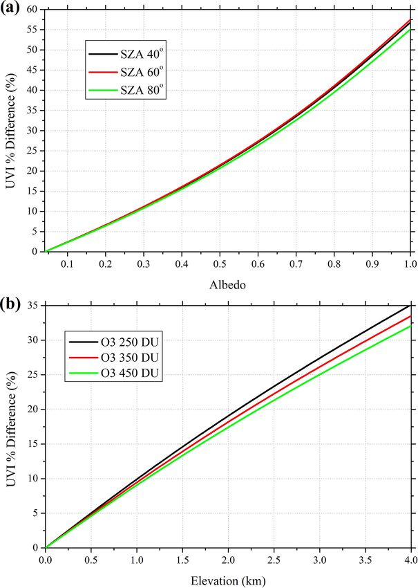
P. G. Kosmopoulos et al.: The UVIOS system: description and quality assessment                                                  5661

Table 1. UVIOS model input parameters.

   Parameter           Description                                 Source                                      Reference
                       (spatial–temporal resolution)
   Cloud               Nowcast cloud optical thickness (COT),      Meteosat Second Generation (MSG4)           MétéoFrance
   microphysics        cloud phase (CPH) (5 km – 15 min)           NOA Antenna                                 (2013)
   Aerosol optical     1 d forecast aerosol optical depth (AOD)    Copernicus Atmosphere Monitoring            Eskes et al. (2015)
   depth               (40 km – 3 h)                               Service (CAMS) – FTP access
   Aerosol optical     Single scattering albedo (SSA), Ångström    Aerosol Comparisons between                 Kinne (2019)
   properties          exponent (AE)                               Observations and Models (Aerocom)
                       (1 × 1◦ – 1 month)
   Solar elevation     Solar zenith angle (SZA)                    Astronomical model                          Reda and Andreas
                       (5 km – 15 min)                             In-house software (NOA)                     (2008)
   Surface albedo      Surface albedo (ALB)                        Copernicus Global Land Service (CGLS)       Carrer et al. (2010)
                       (1 km – 12 d)
   Water vapor         H2 O observation                            Global Ozone Monitoring Experiment 2        Noël et al. (2008)
                       (40 × 80 km – 1 d)                          Level 2 data (GOME-2 L2)
   Surface elevation   Elevation observation (ELE)                 Digital elevation model (DEM)               NOAA (1988)
                       (1 m – fixed)                               In-house database (NOAA)
   Ozone               1 d forecast total ozone column (TOC)       Tropospheric Emission Monitoring Internet   Eskes et al. (2003)
                       (1 × 1◦ – 1 d)                              Service (TEMIS) with Assimilated Ozone
                                                                   Fields from GOME-2 (METOP-B)

tal ozone column (TOC) is at a spatial resolution of 1◦ × 1◦        AE, and SSA) with small step sizes dramatically increased
– 1 d with assimilated ozone fields from the Global Ozone           the LUT size, followed by high computing requirements for
Monitoring Experiment (GOME-2) (METOP-B) (Eskes et                  the multi-parametric interpolation/extrapolation procedures.
al., 2003). We have to mention also here that the selection            For the UVIOS simulations performed in this study, a 32-
of the RTM inputs has been decided based on their real-time         core UNIX server was used equipped with 256 GB of RAM
availability.                                                       and 12 TB of a storage system working in a RAID10 ar-
                                                                    chitecture. The combination of the HPC with the analytical
2.2   Real-time processing concept                                  LUTs, which were developed by using the libRadtran RTM,
                                                                    allows a high-speed multi-parametric interpolation and poly-
The LUT approach, despite its large size (almost 2.5 million        nomial reconstruction (Gal, 1986) to increase accuracy be-
spectral RTM simulations for clear- and all-sky conditions)         tween the LUT records following a mathematical equation
(Kosmopoulos et al., 2018), still provides estimates at dis-        relating the UVIOS outputs to the EO inputs.
crete input parameter values. To overcome this mathematical            An example of the UVIOS input–output data is presented
issue, we performed a multi-parametric interpolation tech-          in Fig. 1 through a flowchart illustration of the modeling
nique to correct the input–output parameter intervals. This         technique scheme. The inputs, including the solar and surface
solution is computationally more costly than a continuous           elevation, albedo, aerosol, ozone forecasts and cloud obser-
function-approximation model, i.e., a neural network (NN)           vations as described in Table 1 are fed to the real-time solver
model (Kosmopoulos et al., 2018), but the accuracy improve-         that results in spectrally weighted output of UVI for the Eu-
ment is significant. Indicatively, using a test set of 1 million    ropean region. Figure 2 shows the memory usage and error
RTM simulations for UVI from the developed LUT, we ap-              statistics for a range of different LUT sizes. The LUT error
plied the NN developed in Kosmopoulos et al. (2018) and             decreases as the LUT size increases, regardless of the func-
found a mean execution time of around 144 s followed by             tion being approximated. The LUT sizes in Fig. 2 fit into the
a mean absolute error (MAE) of 0.0321, while by using the           cache in our HPC environment; thus, performance in terms
proposed UVIOS multi-parametric interpolation exploiting            of processing speed and overall output accuracy vary only
the HPC and distributed computing benefits, we found for            slightly between the table sizes shown. In our case, UVIOS
the same test set an execution time of 295 s with a MAE of          shows that LUT transformation can provide a significant per-
0.0001. The inclusion of many parameters (in this study we          formance increase without incurring an unreasonable amount
incorporated eight, i.e., AOD, SZA, TOC, COT, ELE, ALB,             of error, provided there is sufficient memory available. We

https://doi.org/10.5194/amt-14-5657-2021                                              Atmos. Meas. Tech., 14, 5657–5699, 2021
5662 P. G. Kosmopoulos et al.: The UVIOS system: description and quality assessment
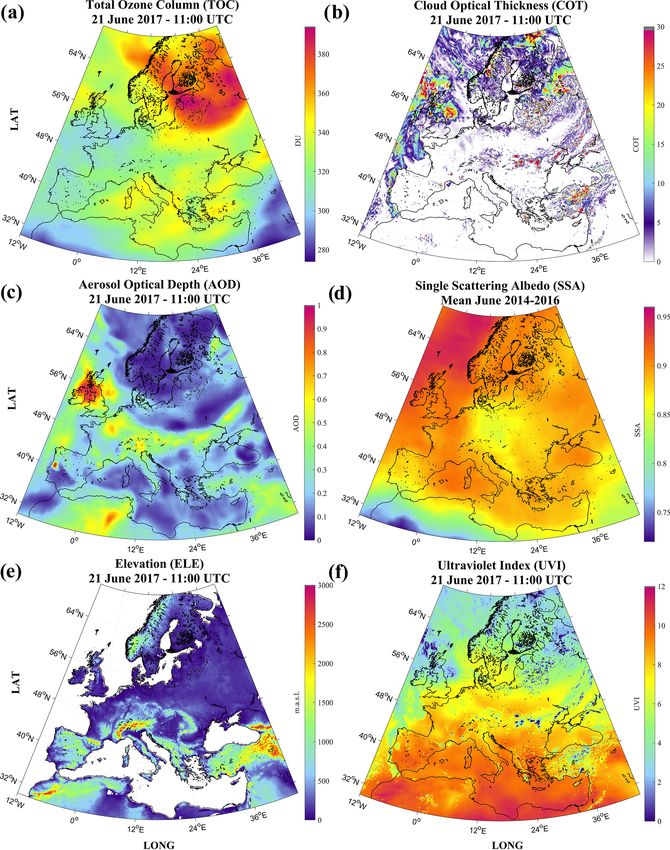
Figure 1. Flowchart illustration of the UVIOS modeling technique scheme. The pre-calculated effects of solar and surface elevation and
albedo followed by the aerosol and ozone forecasts and the real-time cloud observations to the UVIOS solver result in the spectrally weighted
output of UVI for the European region.
ing dimension (i.e., what is happening now) in terms of cloud
microphysics data every 15 min retrieved in real time by the
geostationary satellite MSG. The forecasts represent the fu-
ture estimations (day ahead in our study) of aerosol optical
properties and total ozone column based on deterministic
approaches (European Centre for Medium-Range Weather
Forecasts – ECMWF) and assimilated satellite data for bet-
ter accuracy. As a result, UVIOS under cloudless conditions
operates as a forecast system since it uses forecasted inputs
and provides the clear-sky UVI forecasts operationally. By
adding the nowcast cloud information as input to UVIOS
(i.e., all-sky conditions), the whole procedure will follow the
time steps of MSG cloud microphysics data collocated and
synchronized with the forecast data. So, following the pro-
Figure 2. UVIOS memory usage and error statistics in terms of
mean bias error (MBE) for a range of different LUT sizes. posed operation method of this study, UVIOS can be used as
a UVI forecast system for cloudless conditions or as a UVI
nowcast system for all-sky conditions.
note that the cache size is a critical factor for LUT perfor- 2.3 Input data description
mance, while under a HPC environment practically there is
no limit. Such techniques can be implemented in hardware The COT data from Meteosat was used, whose retrieval al-
with distributed computing that operates in parallel to pro- gorithm is based on 0.6 and 1.6 µm channel radiances of
vide optimum performance. Meteosat’s Spinning Enhanced Visible and InfraRed Imager
Since UVIOS can produce massive UVI outputs of the or- (SEVIRI). MSG products have been described in Derrien
der of 1.5 million simulations in less than 5 min following the and Le Gléau (2005) and the MétéoFrance (2013) techni-
proposed simulation and computing architecture, this means cal report. The COT impact uncertainty in UVI deals with
that it can be used for both operational applications and real- the MSG COT reliability and accuracy and hence introduces
time estimations. The exact use of UVIOS depends only on errors into the UVIOS simulations (Derrien and Le Gléau,
the available input data sources. For this study both nowcasts 2005; Pfeifroth et al., 2016). In addition, comparison princi-
(clouds) and forecasts (ozone, aerosol) were used as inputs to ples of (point) station UVI measurements with a 5 km MSG
the system. The nowcasts represent the continuous monitor- COT matrix are possibly responsible for at least part of the
Atmos. Meas. Tech., 14, 5657–5699, 2021 https://doi.org/10.5194/amt-14-5657-2021
P. G. Kosmopoulos et al.: The UVIOS system: description and quality assessment                                            5663

observed deviations (e.g., Kazadzis et al., 2009a). For in-      albedo of 0.05 for non-snow cases and a UV ALB equal
stance, when a MSG pixel is partly cloudy, the ground mea-       to CGLS when CGLS exceeded 0.5 (snow cover). The total
surements of UVI could fluctuate by more than 100 %, de-         ozone column forecasts were obtained from TEMIS, which
pending on whether the Sun is visible or whether clouds          is a near-real-time service which uses the satellite observa-
attenuate the direct component of the solar irradiance. The      tions of total ozone column by GOME and SCIAMACHY
result is that in cases of partly covered MSG pixels and in      assimilated in a transport model, driven by the ECMWF
the absence of clouds between the ground measurement and         forecast meteorological fields (Eskes et al., 2003). The el-
the Sun, the ground truth UVI would be much higher than          evation data were obtained from the 5 min Gridded Global
the UVIOS one. Of course, the presence of small clouds           Relief Data (ETOPO5) database, which provides land and
which have not been identified by MSG and cover (part of)        seafloor elevation information on a 5 min latitude–longitude
the Sun disk is plausible as well, consequently causing an       grid, with a 1 m precision in the region of Europe, and is
overestimation of the modeled UVI (Koren et al., 2007).          freely available from NOAA (NOAA, 1988). An analytical
Furthermore, sensors onboard geostationary satellites suffer     description of the above geophysical parameters including
from the parallax error, which contributes to the spatial er-    their specifications and resolution can be found in Table 1,
rors of the images and the overall uncertainty of the products   followed by the corresponding references for more techni-
(Bieliński, 2020; Henken et al., 2011). The error depends on    cal details. Figure 3 shows an example of the input–output
the altitude of the cloud and the viewing angle (parallax er-    UVIOS parameters. An extensive validation of the MACC
rors are more significant for high viewing angles).              analysis and forecasting system products was performed by
   UVIOS calculations at high solar zenith angles (> 70◦ )       Eskes et al. (2015). The aerosol optical properties were val-
are retrieved assuming cloudless skies since the MSG COT         idated against 3-year (April 2011–August 2014) near-real-
product is not available in these conditions, facing reliabil-   time level-1.5 AERONET measurements, and for AOD at
ity issues (Kato and Marshak, 2009). This has an effect on       550 nm an overall overestimation was exhibited. Due to ded-
the quality of the UVIOS overall performance at high solar       icated validation activity of the MACC service, a validation
zenith angles, where there is no cloud information as input      report that covers the time period of this study (Eskes et al.,
to the model in order to quantify the consequent impact on       2018) is also available, presenting an overall positive mod-
UVI. However, such measurements under high solar zenith          ified normalized mean bias during 2017, ranging from 0 to
angles are accompanied by very low UVI levels (< 1), both        0.4, with the same range of values over the study region (Eu-
in the performed RTM simulations and in the ground-based         rope). This overestimation of AOD at 550 nm may explain
measurements. This inconsistency, even if does not affect        some of the UVI underestimation under clear-sky conditions
UVIOS UVI results associated with dangerous effects on hu-       (see Sect. 4.2.2).
man health, nevertheless is still affected by the rest of the
input parameters (i.e., ozone, aerosol) mitigating the UVIOS
uncertainty in the absence of cloud information under such       3     Ground measurements and evaluation methodology
high solar zenith angles. There is more discussion in the next
section on how we use these data for the UVIOS validation.       3.1    Ground-based measurements
   For the total aerosol optical depth, we used 1 d forecast
data from CAMS as the basic input parameter. These fore-         In order to validate the UVIOS results, 17 ground-based sta-
casts are based on the Monitoring Atmospheric Composition        tions were selected, for which measurements of the UVI were
and Climate (MACC) analysis and provide accurate data of         available during 2017. The stations are shown in Fig. 4. Com-
AOD at 550 nm with a time step of 1 h and a spatial resolu-      parisons were performed with a 15 min step. The ground-
tion of 0.4◦ . For aerosol single scattering albedo properties   based measurements were obtained from spectrophotometers
climatological values from the MACv2 aerosol climatology         (Brewer), spectroradiometers (Bentham), filter radiometers
(Kinne, 2019) were utilized. Monthly means of single scat-       (GUV) and broadband instruments (SL501 and YES) as Ta-
tering albedo at 310 nm were acquired from global gridded        ble 2 shows. Note that UV data in Table 2 have been cal-
data at a 1◦ × 1◦ spatial resolution. Also, in order to derive   ibrated, processed and provided directly by the responsible
the Ångström exponent, monthly means of AOD at 340 and           scientists for each station. References wherein more infor-
550 nm were used. The calculated Ångström exponent was           mation for the data quality of particular instruments can be
then applied to the 550 nm AOD (from CAMS) in order to           found are also provided. Brewer spectrophotometers measure
get AOD in the UV.                                               the global spectral UV irradiance with a step of 0.5 nm and
   The surface albedo data were obtained from CGLS               a resolution which is approximately 0.5 nm (usually between
(Geiger et al., 2008; Carrer et al., 2010). As a global sur-     0.4 and 0.6 nm). Depending on their type the spectral range is
face ALB product is not available in the UV region, for this     usually 290–325 nm (MKII, MKIV) or 290–363 nm (MKIII).
study we have used the climatological product of CGLS (in        Since Brewer spectrophotometers measure the spectrum up
the visible range) (Lacaze et al., 2013) as follows: based on    to a wavelength which is shorter than 400 nm, extension of
the findings of Feister and Grewe (1995), we used a UV           the spectrum up to 400 nm in order to calculate the UV in-

https://doi.org/10.5194/amt-14-5657-2021                                          Atmos. Meas. Tech., 14, 5657–5699, 2021
5664                                    P. G. Kosmopoulos et al.: The UVIOS system: description and quality assessment

Figure 3. An example of the input TOC (a), COT (b), AOD (c), SSA (d), ELE (e) and output UVI (f) maps based on the UVIOS modeling
technique applied for 21 June 2017 at 11:00 UTC.

dex is usually achieved using empirical methods (e.g., Fi-         recorded with a step of either 0.25 or 0.5 nm and a resolution
oletov et al., 2003; Slaper et al., 1995). The additional un-      of ∼ 0.5 nm. The Brewer spectrophotometer measures the to-
certainty in the UVI due to the latter approximation is well       tal column of ozone using the differential absorption method,
below the overall uncertainty in the measurements. Bentham         i.e., measuring the direct solar irradiance at four wavelengths
spectroradiometers measure the whole UV spectrum (290–             and then comparing the intensity at wavelengths that are
400 nm) with a step and resolution which can be determined         weakly and strongly absorbed by ozone (Kerr et al., 1985).
by the operator. The spectra from AOS and LIN (measured            Brewer TOC measurements are used in the present document
by Bentham spectroradiometers) used in this study have been        to validate the TEMIS forecasts. The Ground-based Ultra-

Atmos. Meas. Tech., 14, 5657–5699, 2021                                             https://doi.org/10.5194/amt-14-5657-2021
P. G. Kosmopoulos et al.: The UVIOS system: description and quality assessment                                           5665

                                                                 3.2   Evaluation methodology

                                                                 The time series period covers the whole year of 2017 at
                                                                 15 min intervals, following the MSG available time steps.
                                                                 A synchronization between the UVIOS simulations and
                                                                 the ground-based measurements was performed in order to
                                                                 match the 15 min intervals of UVIOS to the measured data.
                                                                 The UVIOS data availability is 93 %, while for the ground
                                                                 stations it reaches almost 79 %, enabling a direct UVI data
                                                                 comparison of 77 % of the 2017 time steps. For the com-
                                                                 parison we used the closest instrument measurements to the
                                                                 15 min intervals with a maximum deviation of 3 min in order
                                                                 to avoid solar elevation and cloud presence mismatches. Ad-
                                                                 ditionally, the UVIOS comparisons included measurements
                                                                 up to 70◦ SZA. The rationale for this cutoff was that UVIOS
                                                                 retrievals at high SZA are retrieved as cloudless as COT is
                                                                 unavailable from MSG. In addition, the comparison is also
Figure 4. Study region and UVI ground measurement locations.
                                                                 impacted by limitation of the horizon of ground-based sites
                                                                 (e.g., Davos, Innsbruck, Aosta) where the diffuse component
violet (GUV) instrument is a multichannel radiometer that        and in some cases the direct component of solar UV irradi-
measures UV radiation in five spectral bands having central      ance are affected by obstacles (mountains) on the horizon.
wavelengths as 305, 313, 320, 340 and 380 nm. However, in        The contribution of this mainly diffuse irradiance to the to-
addition to UV irradiances, other data that can be obtained      tal budget is a function of solar elevation and azimuth (day
from GUV instruments are total ozone and the cloud optical       of the year) and also cloudiness. Although UVIOS simula-
depth (Dahlback, 1996; Lakkala et al., 2018). GUV measure-       tions were corrected for changing UVI with respect to alti-
ments are used for the LAN station of Norway. At stations        tude (see Sect. 3.2.3), the correction cannot be perfect for
AKR, INN and VIE, the surface UV was measured using So-          higher-altitude stations. The reason is that it is not possi-
lar Light (SL) 501 radiometers. It provides direct observation   ble to take into account all different factors (aerosol load
of the UV index with a frequency of 1 min. The Yankee Envi-      and properties, atmospheric pressure, surface albedo) (e.g.,
ronmental System (YES) has been used for the VAL station.        Blumthaler et al., 1997; Chubarova et al., 2016) which affect
   The low-latitude stations include AKR, ARE, ATH, ROM,         the change in UVI with altitude. This explains some of the
THE, and VAL. AKR has a minimum altitude of 23 m and             deviations in the results as UVIOS retrieves UVI assuming a
VAL has a maximum altitude of 705 m above sea level. The         flat horizon. Clear-sky conditions were defined as the UVIOS
middle-latitude locations are AOS, DAV, INN, BEL, LIN,           retrieval where MSG COT equals zero. Further discussion on
MAN, UCC, and VIE, among which the minimum altitude              the uncertainties introduced by this choice is mentioned in
is 10 m in LAN and maximum altitude is in DAV at 1610 m          the cloud effect section.
above mean sea level. HEL, LAN, and SOD represent the               Most of the comparisons have been performed
high-latitude zone, with HEL having an altitude of 48 m and      using the absolute (mean bias or median) UVI
SOD an altitude of 185 m above mean sea level (Table 2).         differences       (model − measurements).        In     addi-
A summary of basic climatic information for the validation       tion, median values of the percentage differences
locations was obtained from the Köppen climate classifica-       (100 × (model − measurements) / measurements)            have
tion (Chen and Chen, 2013), and it is summarized here. THE,      been used. UVIOS estimations were also evaluated in terms
AKR, ARE, ROM, ATH and VAL have a Mediterranean cli-             of mean bias and root mean square error (MBE and RMSE,
mate comprising mild, wet winters and dry summers. MAN           respectively), defined as follows:
experiences a maritime climate (cool summer and cool, but                         N
                                                                               1 X
not very cold, winter). AOS, UCC, LAN, BEL, HEL, LIN             MBE = ε =           εi ,                                   (1)
and VIE experience a humid continental climate with warm                       N i=1
to hot summers, cold winters and precipitation distributed
                                                                           r
                                                                               1 XN 2
throughout the year. DAV and INN experience boreal climate       RMSE =              ε ,
                                                                                  i=1 i
                                                                                                                            (2)
                                                                               N
characterized by long, usually very cold winters and short,
cool to mild summers. SOD has a subarctic climate with very      where εi = xf − xo are the residuals (UVIOS errors), calcu-
cold winters and mild summers.                                   lated as the difference between the simulated values (xf ) and
                                                                 the ground-based values (xo ), and where N is the total num-
                                                                 ber of values. MBE quantifies the overall bias and detects
                                                                 whether UVIOS overestimates (MBE > 0) or underestimates

https://doi.org/10.5194/amt-14-5657-2021                                           Atmos. Meas. Tech., 14, 5657–5699, 2021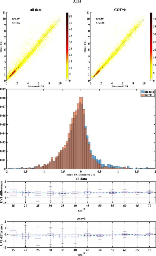
5666 P. G. Kosmopoulos et al.: The UVIOS system: description and quality assessment
Table 2. Coordinates (degrees), instrument type, height (meters above sea level) and maximum UVI-measured levels of the European stations
used for the comparison.
Station Country Code Latitude Longitude Instrument Height UVI max Reference
(◦ N) (◦ E) (m a.s.l.)
Akrotiri Cyprus AKR 34.59 32.99 SL501 23 9.14
Aosta Italy AOS 45.74 7.36 Bentham DTMc300 570 9.60 Fountoulakis et al. (2020b)
El Arenosillo Spain ARE 37.10 −6.73 Brewer MKIII 52 9.78
Athens Greece ATH 37.99 23.78 Brewer MKIV 180 10.20
Belsk Poland BEL 51.84 20.79 Brewer MKIII 176 7.54 Czerwińska et al. (2016)
Davos Switzerland DAV 46.81 9.84 Brewer MKIII 1590 10.57
Helsinki Finland HEL 60.20 24.96 Brewer MKIII 48 5.68 Lakkala et al. (2008)
Innsbruck Austria INN 47.26 11.38 SL501 577 8.35 Hülsen et al. (2020)
Landvik Norway LAN 58.33 8.52 GUV-541 10 6.65 Johnsen et al. (2008)
Lindenberg Germany LIN 52.21 14.11 Bentham DTMc300 127 8.86
Manchester UK MAN 53.47 −2.23 Brewer MKII 76 7.30 Smedley et al. (2012)
Rome Italy ROM 41.90 12.50 Brewer MKIV 75 8.38
Sodankyla Finland SOD 67.37 26.63 Brewer MKIII 179 4.51 Heikkilä et al. (2016),
Lakkala et al. (2008)
Thessaloniki Greece THE 40.63 22.96 Brewer MKIII 60 10.40 Fountoulakis et al. (2016),
Garane et al. (2006)
Uccle Belgium UCC 50.80 4.35 Brewer MKIII 100 8.99 De Bock et al. (2014)
Valladolid Spain VAL 41.66 −4.71 YES 705 10.32 Hülsen et al. (2020)
Vienna Austria VIE 48.26 16.43 SL501 153 8.09 Hülsen et al. (2020)
(MBE < 0). RMSE quantifies the spread of the error distri- tion coefficients are between 0.85 and 0.99 for all the sta-
bution. Finally, the correlation coefficient (r) as well as the tions. The RMSE is for most stations less than 0.5. Under
coefficient of determination (R 2 ) were used to represent the all-sky conditions the RMSE is higher relative to the RMSE
proportion of the variability between modeled and measured for clear skies for MAN, DAV and SOD, which is proba-
values. bly due to misclassification of cloudy pixels (see also Ap-
pendix A). Relative differences can be misleading as they
may correspond to very small absolute differences without
4 Results physical meaning, especially for low levels of the UVI. Thus,
we focused on absolute differences in order to have a more
4.1 Overall performance of the UVIOS system representative assessment of the actual effect (UV index)
and its results. The differences were categorized as low (less
Figure 5 presents a density scatterplot of the UVIOS simula- than 0.5), moderate (0.5–1) and high (more than 1). In Ap-
tions for all stations as compared to the ground-based mea- pendix A, relative differences are also discussed.
surements, in which a pattern of shaded squares represents In Table 3, U1.0 and U0.5 represent the percentage
the counts of the points falling in each square and which of cases with absolute differences between modeled and
shows a correlation coefficient (r) of 0.94. For a more de- ground-based UVI measurements within 1 and 0.5, respec-
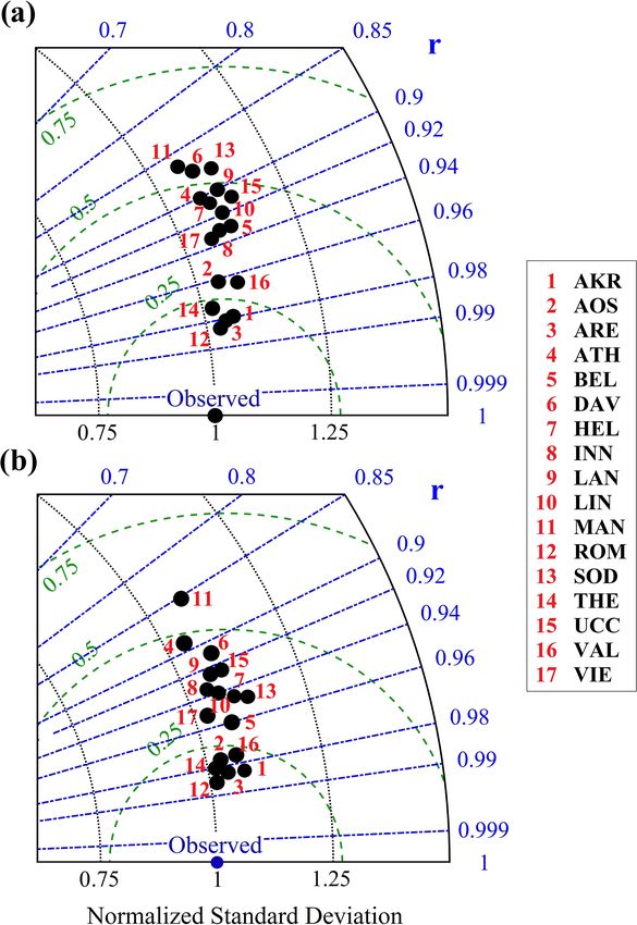
tailed view of the UVIOS performance, Fig. 6 depicts a Tay- tively, for all comparisons between the 15 min model re-
lor diagram with the overall model accuracy for all ground trievals and the corresponding ground-based measurements.
stations under all-sky and clear-sky conditions as a function As shown in Table 3, for all stations and for both clear- and
of the correlation coefficient, normalized standard deviation all-sky conditions, differences were within 0.5 UVI for at
and RMSE. For both clear-sky and all-sky conditions, the re- least 70 % of the cases. Under clear-sky conditions, AOS,
sults are similar. The absolute differences between UVIOS BEL, HEL, LAN, LIN, SOD and THE had above 90 % of
and the measured UVI are within ±0.5, and the correla- U0.5 cases, while others had 75 %–90 % of U0.5 cases. All
Atmos. Meas. Tech., 14, 5657–5699, 2021 https://doi.org/10.5194/amt-14-5657-2021P. G. Kosmopoulos et al.: The UVIOS system: description and quality assessment 5667
Table 3. Absolute difference between UVIOS and ground-based
UVI measurements in terms of percentages (%) of data that are
within 0.5 and 1 UVI of difference (U0.5 and U1.0, respectively)
as well as the correlation coefficient (r) for all-sky and clear-sky
conditions.
Station All sky Clear sky
U0.5 U1.0 r U0.5 U1.0 r
AKR 82.25 96.02 0.980 84.57 97.48 0.987
AOS 86.81 94.40 0.961 92.23 97.07 0.978
ARE 85.15 95.73 0.981 87.99 96.86 0.986
ATH 84.99 94.29 0.902 88.98 96.35 0.891
BEL 83.07 93.28 0.933 91.30 96.50 0.960
DAV 74.20 86.43 0.873 76.19 87.06 0.912
HEL 86.53 94.79 0.909 94.13 97.70 0.944
INN 79.96 92.17 0.932 87.09 95.23 0.937
LAN 84.94 93.46 0.900 92.34 96.52 0.925
Figure 5. Density scatterplot of the overall UVIOS performance for LIN 81.58 91.86 0.919 90.95 96.31 0.941
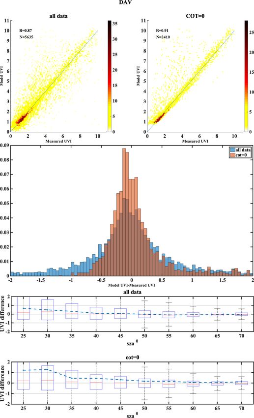
all stations. The analytical statistics for each station can be found in MAN 77.72 90.44 0.862 87.85 94.27 0.852
Appendix A. ROM 87.69 96.19 0.985 89.55 97.00 0.991
SOD 90.86 97.26 0.883 95.69 98.94 0.947
THE 88.98 95.91 0.974 92.51 97.35 0.981
UCC 71.18 87.68 0.913 83.23 92.15 0.926
VAL 85.86 93.93 0.962 86.61 95.22 0.976
VIE 76.65 91.53 0.936 83.37 94.42 0.952
cases for all stations, with the correlation coefficients ex-
ceeding 0.9 for most of them (exceptions are DAV, MAN
and SOD). Median differences for all skies for every station
were well within ±0.2 UVI, with the 25th–75th percentiles
being within ±0.5 UVI and the 5th–95th percentiles within
±1 UVI. For clear skies the corresponding values are ±0.1,
±0.4 and ±0.8, respectively. In the following sections we try
to investigate the factors that contribute to the differences be-
tween UVIOS and ground-based measurements.
4.2 Factors affecting UVIOS retrievals
4.2.1 Ozone effect
All the available collocated TOC measurements for the sta-
tions used in the UVIOS evaluation have been obtained from
the WOUDC (https://woudc.org/, last access: 22 October
2020) database. In this database 8 out of 17 UVIOS evalu-
ation stations (AOS, ATH, DAV, MAN, ROM, SOD, THE
and UCC) were found, providing TOC ground-based mea-
surements. TOC comparison has been performed by calcu-
Figure 6. Taylor diagram for the overall UVIOS accuracy for all lating daily means of ground-based measurements and the
ground stations under all-sky (a) and clear-sky (b) conditions. TOC from TEMIS. In order to quantify the effect of the un-
certainty of the forecasted TOC used as input at UVIOS, we
have calculated the mean differences of the forecasted and
stations but DAV had above 90 % of U1.0 cases for clear measured TOCs and used a radiative transfer model to in-
skies, while the correlation coefficients for most of the sta- vestigate their effect on the UVIOS-retrieved UVI. Table 4
tions were above 0.9 (exceptions are ATH and MAN). For shows the mean differences in DU from TEMIS TOC (used
all skies differences were within 1 UVI for 90 % of the as inputs in UVIOS) as compared to the WOUDC ground-
https://doi.org/10.5194/amt-14-5657-2021 Atmos. Meas. Tech., 14, 5657–5699, 20215668 P. G. Kosmopoulos et al.: The UVIOS system: description and quality assessment
our total of 17 stations (AKR, ARE, ATH, DAV, HEL, LIN,
ROM, SOD, THE, UCC, VAL and VIE). AERONET (level 2,
version 3) values of AOD at 500 nm were interpolated at
550 nm using the AERONET-derived 440–870 nm Ångström
exponent for each individual measurement. In order to com-
pare those measurements with CAMS-forecasted AOD used
for UVIOS, their daily means were derived. The compari-
son of forecasted and measured daily means was based on
all available data due to gaps in the AERONET time series.
The AOD MBE and RMSE statistical scores are shown in
Table 5 in absolute units and correlation coefficient as well.
All the stations have a mean positive bias up to 0.071 except
UCC, which shows a mean negative bias of 0.007. The com-
Figure 7. Differences of UVI derived by UVIOS using as input the parison of all individual stations with CAMS data used as
TEMIS and Brewer TOC, respectively, at all stations with available inputs on UVIOS showed that under all cases CAMS AOD
data (lower possible SOD SZA is 44◦ ).
is higher than that from AERONET with a mean difference
of 0.07 at 550 nm. The correlation between the modeled and
based measurements for 1 year of comparison data. It is seen measured values varies from 0.10 for VIE to 0.91 for ARE,
that for the stations AOS, DAV, MAN and UCC the values with most of the stations showing the correlation coefficient
of the TEMIS observations are higher as compared to the above 0.7. As in the case of the TOC, AOD CAMS data are
ground-based measurements (by 7.6, 1.9, 5, and 2.9 DU, re- forecasts from the previous day and real-time WOUDC or
spectively), while for the other stations TEMIS observations AERONET level 2.0 data do not exist. Although real-time
are lower (by 0.9, 5.4, 9.9, and 2.2 DU for ATH, ROM, SOD, TOC (and in due course AOD in the UV) is available from
and THE, respectively). The negative bias is seen to be high- Eubrewnet (López-Solano et al., 2018; Rimmer et al., 2018),
est for the ROM station (−9.9), and the positive bias is high- it is only for particular locations and not for the whole Euro-
est for the AOS station (7.6). Part of the large differences pean domain. Thus, the only choice in providing for a real-
over the complex terrain sites can be explained by the differ- time UV index for Europe is using the CAMS (for AOD) and
ence between the actual altitude of the station and the average TEMIS (for TOC) data.
altitude of the corresponding grid points of TEMIS. For ex- In order to evaluate the effect of AOD on UVI, UVI differ-
ample, for AOS the average altitude of the pixel is 2000 m, ences between the UVIOS using both AOD data sets (CAMS
while the real altitude of the station is 570 m, resulting in and AERONET) as UVIOS inputs were analyzed. Figure 8
an underestimation of the tropospheric column of ozone by shows the mean bias error of the CAMS–AERONET AOD
TEMIS. In general, differences can be explained by the com- impact on UVI for all stations with available ground-based
bined effects of uncertainties in TOC retrieval from satellite AOD data as a function of SZA together with the uncer-
and ground-based platforms (Rimmer et al., 2018; Boynard tainty range (±1σ ). It can be seen that UVIOS with CAMS
et al., 2018; Garane et al., 2018). Figure 7 shows the effect of AOD input underestimates UVI compared to UVIOS with
this TOC bias on the calculated UVIOS. As seen in Table 4, AERONET data, except for the UCC station. This is consis-
there is a mix of small underestimation and overestimation tent with CAMS overestimations of AOD compared to the
cases in the TOCs used within UVIOS, with average abso- AERONET measurements, except for the UCC station as
lute differences of 4–5 DU. The worst TOC UVIOS inputs shown in Table 5. Higher aerosol levels in the atmosphere
were found in AOS and ROM (7.6 and −9.9 DU), leading tend to lower the UVI. The highest difference in UVI is ob-
to maximum (at 30◦ SZA) differences in UVI of −0.22 and served for the stations HEL, SOD, and VIE. Since the aerosol
0.3 for AOS and ROM, respectively. In general, in most of level at the stations HEL and SOD is very low, the percent
the cases UVI mean differences are less than 0.1. It has to difference between the AOD from CAMS and AERONET
be noted that the TOC differences have a larger impact when is larger for these stations (although the absolute difference
expressed in percent at higher SZAs, while in Fig. 7 higher is similar) relative to stations with higher AOD, leading to
absolute differences for low SZAs are associated with higher higher differences in the UVI. Aerosol content for VIE is
UVIs at these SZAs. Detailed comparisons for each station higher than HEL and SOD but still within 0.2, which might
are shown in the Appendix A figures. be the reason for the higher UVI difference. In terms of SZA,
it is observed that the mean bias decreases with an increase
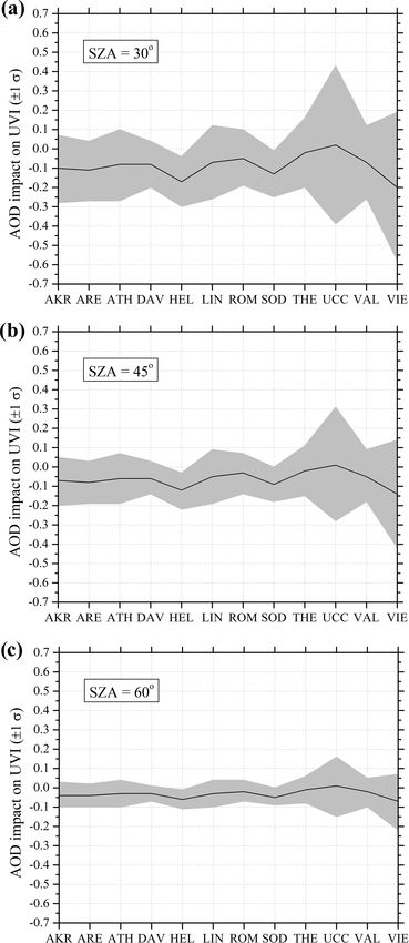
4.2.2 Aerosol effect in the SZA as the values of UVI also decrease with SZA, and
the most deviation is for station VIE, which is consistent with
Aerosol optical depth measurements used for the UVIOS the poor correlation between the CAMS-forecasted input and
aerosol input evaluation have been collected from the the measurements for this station as seen from Table 5.
AERONET-NASA web site (Giles et al., 2019) for 12 out of
Atmos. Meas. Tech., 14, 5657–5699, 2021 https://doi.org/10.5194/amt-14-5657-2021P. G. Kosmopoulos et al.: The UVIOS system: description and quality assessment 5669
Table 4. Mean bias error of the TEMIS TOC as compared to the WOUDC ground-based measurements.
Station AOS ATH DAV MAN ROM SOD THE UCC
MBE TOC (DU) 7.6 −0.9 1.9 5.0 −9.9 −5.4 −2.2 2.9
RMSE TOC (DU) 15.8 10.0 9.1 11.3 12.5 13.1 6.2 7.8
r 0.92 0.95 0.97 0.97 0.94 0.97 0.99 0.98
Table 5. Comparison results between CAMS-forecasted AOD values used as UVIOS input and AERONET ground-based AOD measure-
ments. The AOD MBE and RMSE statistical scores are shown in absolute units along with the correlation coefficient.
Station AKR ARE ATH DAV HEL LIN ROM SOD THE UCC VAL VIE
MBE 0.037 0.042 0.030 0.029 0.062 0.026 0.017 0.047 0.008 −0.007 0.024 0.071
RMSE 0.074 0.070 0.074 0.053 0.078 0.074 0.056 0.065 0.066 0.150 0.073 0.157
r 0.77 0.91 0.80 0.73 0.70 0.69 0.80 0.63 0.76 0.50 0.78 0.10
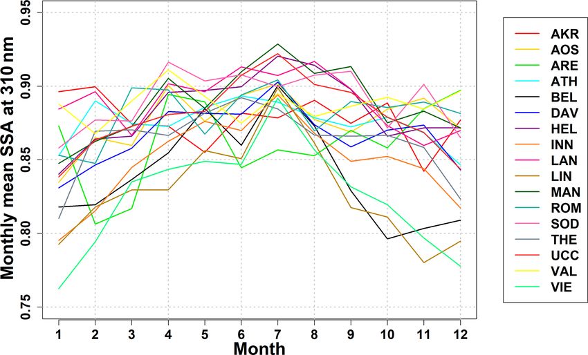
The use of single scattering albedo in the UV region is a age difference is independent of the SZA and increases with
difficult task, and many studies have shown that such mea- surface albedo. The UVI percentage difference is found also
surements need extra effort, and it is not possible to perform to increase almost linearly with the increase in elevation for
them worldwide (Arola et al., 2009; Kazadzis et al., 2016; a particular total ozone column. The percentage difference is
Raptis et al., 2018). The monthly values of the single scatter- similar for all ozone columns up to 1 km, after which the dif-
ing albedo used in UVIOS for the UV region were derived ferences with ozone column become more apparent. That is,
from the MACv2 database at the 310 nm wavelength (Kinne, at a particular elevation, the percentage difference is higher
2019). Figure 9 shows the intra-annual variability of SSA for for less total ozone column. A 1 % fluctuation (decline or in-
the 17 stations. For all stations, SSA values range from 0.76 crease) in column ozone can lead to about a 1.2 % fluctuation
to 0.93, with most of them having SSA values between 0.83 (increase or decline) in the UV index (Fioletov et al., 2003;
and 0.93 and relatively small variability. In contrast, there are Probst et al., 2012). Indicatively, the average maximum sur-
stations like ARE, BEL, INN, LIN, VIE and THE which have face elevation correction in terms of UVI for the DAV station
relatively smaller SSA values (0.76–0.9) and greater variabil- (due to UVIOS input deviation from the actual elevation) was
ity than the other stations. on the order of 1.6 (15 %), while for INN and AOS it was 0.5
and 0.6, respectively (6 %), and for the VAL station close to
4.2.3 Albedo effect and surface elevation correction 0.8 (8 %).
Uncertainties introduced in UVIOS from the use of a con-
Surface albedo at UV wavelengths is small (2 %–5 %) for stant surface albedo value of 0.05 for non-snow conditions
most types of surfaces (Feister and Grewe, 1995; Madronich, are quite low. For the case of albedo values used for snow
1993) except for features like sand (with a typical albedo conditions based on the CGLS monthly mean product, uncer-
of ∼ 0.3) and snow (up to 1 for fresh snow) (Meinander et tainties can be related to the small difference of UV and visi-
al., 2013; Myhre and Myhre, 2003; Vanicek et al., 2000; ble albedo values; the fact that the CGLS provides an albedo
Henderson-Sellers and Wilson, 1983). Renaud et al. (2000) of a certain area around the station that does not necessar-
found an enhancement of about 15 % to 25 % in UVI for ily coincide with the “effective” albedo area affecting UV
clear skies and snow conditions due to the multiple ground– measurements; and finally that the monthly albedo product
atmosphere reflections, and this relative increment was about represents a monthly average, while a real-time CGLS prod-
80 % larger for overcast conditions. The combined effect of uct represents the last 12 d (dynamically changing albedo).
aerosols and snow led to an enhancement of about 50 % in In order to investigate this last point, we have compared the
UVI in cloud-free conditions for moderately polluted atmo- UV effects from the use of the two albedo data sets for the
spheres (Badosa and Van Weele, 2002). Figure 10a presents DAV station, where the average difference between an ex-
the effect of surface albedo on the UVI percentage difference ample ground-based data set and UVIOS was found to be
(i.e., for various albedo values under clear-sky conditions) as 0.14 UVI (Gröbner, 2021). In Fig. 11, the effect of surface
a function of SZA, while Fig. 10b shows the effect of surface albedo correction is shown for the Davos station for a pe-
elevation on UVI as a function of the percentage difference riod with snow cover and low-percentage cloudiness. The
for various total ozone columns. It is observed that the UVI climatological and dynamically changing albedos are pre-
percentage difference increases almost linearly with albedo sented in terms of percentage differences between modeled
for a particular SZA, and the variation is found to be almost and ground measurements as a function of SZA. In the case
identical for all SZAs. This indicates that the UVI percent-
https://doi.org/10.5194/amt-14-5657-2021 Atmos. Meas. Tech., 14, 5657–5699, 2021You can also read