Aircraft-based measurements of High Arctic springtime aerosol show evidence for vertically varying sources, transport and composition
←
→
Page content transcription
If your browser does not render page correctly, please read the page content below
Atmos. Chem. Phys., 19, 57–76, 2019
https://doi.org/10.5194/acp-19-57-2019
© Author(s) 2019. This work is distributed under
the Creative Commons Attribution 4.0 License.

Aircraft-based measurements of High Arctic springtime
aerosol show evidence for vertically varying sources,
transport and composition
Megan D. Willis1,a , Heiko Bozem2 , Daniel Kunkel2 , Alex K. Y. Lee3 , Hannes Schulz4 , Julia Burkart5 ,
Amir A. Aliabadi6 , Andreas B. Herber4 , W. Richard Leaitch7 , and Jonathan P. D. Abbatt1
1 Department   of Chemistry, University of Toronto, Toronto, Ontario, Canada
2 Institutefor Atmospheric Physics, Johannes Gutenberg University of Mainz, Mainz, Germany
3 Department of Civil and Environmental Engineering, National University of Singapore, Singapore
4 Alfred Wegener Institute, Helmholtz Center for Polar and Marine Research, Bremerhaven, Germany
5 Faculty of Physics, Aerosol Physics and Environmental Physics, University of Vienna, Vienna, Austria
6 School of Engineering, University of Guelph, Guelph, Ontario, Canada
7 Environment and Climate Change Canada, Toronto, Ontario, Canada
a now at: Chemical Sciences Division, Lawrence Berkeley National Laboratory, Berkeley, California, USA

Correspondence: Megan D. Willis (megan.willis@mail.utoronto.ca)

Received: 22 June 2018 – Discussion started: 24 August 2018
Revised: 10 December 2018 – Accepted: 11 December 2018 – Published: 3 January 2019

Abstract. The sources, chemical transformations and re-          masses at the lowest potential temperatures, in the lower po-
moval mechanisms of aerosol transported to the Arctic are        lar dome, had spent long periods (> 10 days) in the Arc-
key factors that control Arctic aerosol–climate interactions.    tic, while air masses in the upper polar dome had entered
Our understanding of sources and processes is limited by a       the Arctic more recently. Variations in aerosol composition
lack of vertically resolved observations in remote Arctic re-    were closely related to transport history. In the lower polar
gions. We present vertically resolved observations of trace      dome, the measured sub-micron aerosol mass was dominated
gases and aerosol composition in High Arctic springtime,         by sulfate (mean 74 %), with lower contributions from rBC
made largely north of 80◦ N, during the NETCARE cam-             (1 %), ammonium (4 %) and OA (20 %). At higher altitudes
paign. Trace gas gradients observed on these flights defined     and higher potential temperatures, OA, ammonium and rBC
the polar dome as north of 66–68◦ 300 N and below poten-         contributed 42 %, 8 % and 2 % of aerosol mass, respectively.
tial temperatures of 283.5–287.5 K. In the polar dome, we        A qualitative indication for the presence of sea salt showed
observe evidence for vertically varying source regions and       that sodium chloride contributed to sub-micron aerosol in the
chemical processing. These vertical changes in sources and       lower polar dome, but was not detectable in the upper po-
chemistry lead to systematic variation in aerosol composition    lar dome. Our observations highlight the differences in Arc-
as a function of potential temperature. We show evidence for     tic aerosol chemistry observed at surface-based sites and the
sources of aerosol with higher organic aerosol (OA), ammo-       aerosol transported throughout the depth of the Arctic tropo-
nium and refractory black carbon (rBC) content in the upper      sphere in spring.
polar dome. Based on FLEXPART-ECMWF calculations, air
masses sampled at all levels inside the polar dome (i.e., po-
tential temperature < 280.5 K, altitude
58                                                                                     M. D. Willis et al.: Spring Arctic aerosol

1    Introduction                                                    on particles can decrease their ability to act as ice-nucleating
                                                                     particles (INPs), leading to larger, more readily precipitat-
Arctic regions are warming faster than the global average,           ing ice crystals (Blanchet and Girard, 1994, 1995). This pro-
with significant impacts on local ecosystems and local people        cess can lead to enhanced atmospheric dehydration, leading
(e.g, Bindoff et al., 2013; Hinzman et al., 2013). While Arc-        to diminished long-wave forcing (Curry and Herman, 1985;
tic warming is driven largely by increasing concentrations of        Blanchet and Girard, 1994, 1995). Further, particles contain-
anthropogenic greenhouse gases and local feedback mecha-             ing mineral dust, organic species, sea salt or neutralized sul-
nisms, short-lived climate forcing agents also impact Arctic         fate can act as ice nuclei and increase ice crystal number,
climate. In particular, short-lived species such as aerosol, tro-    also leading to impacts on long-wave and short-wave cloud
pospheric ozone and methane are important climate forcers            forcing (Sassen et al., 2003; Abbatt et al., 2006; Baustian
(e.g., Law and Stohl, 2007; Quinn et al., 2008). The impact of       et al., 2010; Wagner et al., 2018). Finally, Arctic pollution
pollution aerosol, transported northward over long distances,        aerosol can impact the micro-physical properties of liquid-
on Arctic climate has been significant. For example, a large         containing clouds, by increasing liquid water path and de-
fraction of greenhouse-gas-induced warming (∼ 60 %) has              creasing droplet radius. Such micro-physical changes can re-
been offset by anthropogenic aerosol over the past century,          sult in enhanced long-wave warming effects during winter
such that reductions in sulfur emissions in Europe since 1980        and spring (Garrett and Zhao, 2006; Lubin and Vogelmann,
can explain a large amount of Arctic warming since that time         2006; Zhao and Garrett, 2015).
(∼ 0.5 K) (Fyfe et al., 2013; Najafi et al., 2015; Navarro et al.,      Observations at Arctic ground-based monitoring stations
2016). These estimates are compelling, and at the same time          form the basis of our current knowledge about Arctic aerosol
global models that form the basis of our predictive capabil-         seasonality, chemical composition and sources. These long-
ity often struggle to reproduce key characteristics of Arctic        term observations have demonstrated a pronounced seasonal
aerosol, such as the seasonal cycle and vertical distribution        cycle in Arctic aerosol mass concentrations, particle size
(Shindell et al., 2008; Emmons et al., 2015; Monks et al.,           distribution and composition, driven by seasonal variations
2015; Eckhardt et al., 2015; Arnold et al., 2016). Our incom-        in northward long-range transport and aerosol wet removal
plete understanding of Arctic aerosol processes results in di-       (e.g., Quinn et al., 2007; Sharma et al., 2013; Tunved et al.,
verse and frequently poor model skill in simulating Arctic           2013; Croft et al., 2016; Asmi et al., 2016; Nguyen et al.,
aerosol both at the surface and through the troposphere, and         2016; Freud et al., 2017; Leaitch et al., 2018). Aerosol mass
therefore also in accurately simulating aerosol–climate inter-       concentrations peak in winter to early spring when long-
actions (Arnold et al., 2016). This challenge arises in part due     range-transported accumulation mode particles (200–400 nm
to a lack of vertically resolved observations in Arctic regions.     mode diameter), referred to broadly as “Arctic haze”, dom-
   Particle composition drives aerosol optical properties (e.g.,     inate the particle size distribution (e.g., Croft et al., 2016;
Boucher and Anderson, 1995; Jacobson, 2001; Wang et al.,             Freud et al., 2017). A mixture of natural and anthropogenic
2008), ice nucleation efficiency (e.g., Abbatt et al., 2006;         aerosol is transported to Arctic regions by near-isentropic
Hoose and Möhler, 2012), and heterogeneous chemistry that            transport along surfaces of constant potential temperature
impacts both gas and particle composition (e.g., Fan and Ja-         that slope upwards toward the Arctic (Klonecki et al., 2003;
cob, 1992; Mao et al., 2010; Abbatt et al., 2012). The vertical      Stohl, 2006). The sloping isentropic surfaces form a closed
distribution of aerosol and its chemical and physical proper-        “dome” over the polar region; this polar dome is zonally
ties can impact Arctic regional climate in a number of ways.         asymmetric, extends further south in winter and contracts
First, absorption of incoming solar radiation by aerosol (e.g.,      northward in spring to summer (Shaw, 1995; Law and Stohl,
black carbon) can lead to warming in the lower troposphere           2007; Stohl, 2006; Law et al., 2014).
when present near the surface. In contrast, absorbing aerosol           Arctic haze observed near the surface is largely acidic sul-
present at higher altitudes causes cooling at the surface and        fate, with fewer contributions from organic aerosol (OA),
impacts atmospheric stratification (Rinke et al., 2004; Rit-         dust, nitrate, ammonium and sea salt (Li and Winchester,
ter et al., 2005; Treffeisen et al., 2005; Shindell and Falu-        1989; Quinn et al., 2002, 2007; Shaw et al., 2010; Leaitch
vegi, 2009; Engvall et al., 2009). Further, the location in          et al., 2018). Aerosol acidity increases during winter and
the troposphere impacts deposition to high albedo surfaces,          reaches a peak in late spring (Sirois and Barrie, 1999; Toom-
depending on the mechanism of removal (e.g., Macdonald               Sauntry and Barrie, 2002), before the return of wet removal
et al., 2017). Absorbing aerosol deposited to the surface has        brings the Arctic toward near-pristine conditions with more
a strong impact on the albedo of ice and snow, efficiently           neutralized aerosol (Engvall et al., 2008; Browse et al., 2012;
leading to warming (Clarke and Noone, 1985; Hansen and               Breider et al., 2014; Wentworth et al., 2016; Croft et al.,
Nazarenko, 2004; Flanner et al., 2009; Flanner, 2013). Sec-          2016). Sea salt is thought to be an important contributor to
ond, neutralization of acidic sulfate impacts aerosol water          Arctic haze in winter to early spring owing to stronger wind
content and aerosol phase, with implications for the magni-          speeds over nearby oceans, potential wind-driven sources in
tude of aerosol–radiation interactions (Boucher and Ander-           ice and snow-covered regions, and open leads (Leck et al.,
son, 1995; Wang et al., 2008). Third, sulfuric acid coatings         2002; Shaw et al., 2010; May et al., 2016; Huang and Jaeglé,

Atmos. Chem. Phys., 19, 57–76, 2019                                                      www.atmos-chem-phys.net/19/57/2019/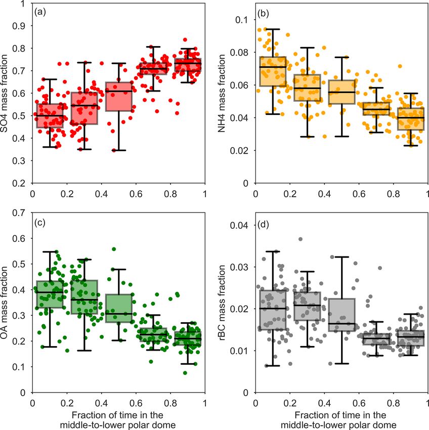
M. D. Willis et al.: Spring Arctic aerosol                                                                                      59

2017; Kirpes et al., 2018). The major source region of near-      using 10-day backward trajectories (e.g, Brock et al., 2011;
surface Arctic haze in winter and early spring is north-          Qi et al., 2017; Leaitch et al., 2018).
ern Europe and northern Asia/Siberia, but the magnitudes             Our knowledge of the vertical distribution of Arctic
of sources in this region have been decreasing in recent          aerosol source regions has also been extended by recent air-
decades (Barrie and Hoff, 1984; Sharma et al., 2004; Koch         borne observations. Results from modelling efforts generally
and Hansen, 2005; Sharma et al., 2006; Hirdman et al., 2010;      agree that Arctic pollution aerosol is a result of a combination
Huang et al., 2010b; Gong et al., 2010; Bourgeois and Bey,        of anthropogenic and natural sources from mid-latitudes in
2011; Stohl et al., 2013; Sharma et al., 2013; Monks et al.,      the Northern Hemisphere; particularly a combination of Eu-
2015; Qi et al., 2017). Surface-based observations have pro-      ropean, north and south Asian, and North American source
vided substantial insight into Arctic aerosol processes, but      regions (e.g., Law et al., 2014; Arnold et al., 2016). How-
owing to the stability of the troposphere the surface can be      ever, modelling efforts provide less quantitative agreement
decoupled from the atmosphere above. Therefore, surface-          on the magnitude of the contributions of each region near
based observations may not represent the overall composi-         the surface and as a function of altitude. Our emerging un-
tion of aerosol transported to the Arctic troposphere (e.g.,      derstanding is of northern Eurasian sources dominating near
Stohl, 2006; McNaughton et al., 2011). How transported            the surface in winter, while North America and southern
aerosol present throughout the troposphere is related to Arc-     and eastern Asia can be important in the middle to upper
tic haze observed near the surface remains an unresolved          troposphere (e.g., Koch and Hansen, 2005; Shindell et al.,
question (Law et al., 2014; Arnold et al., 2016).                 2008; Huang et al., 2010a; Law et al., 2014; Liu et al., 2015;
   Vertically resolved observations of the Arctic atmosphere,     Arnold et al., 2016; Qi et al., 2017). In spring, as the polar
in the last 20 years, have furthered our understanding of the     dome recedes northward, North American and Asian sources
properties, processes, and impacts of Arctic aerosol. Some        become more important at all altitudes (Koch and Hansen,
of the only seasonal airborne observations of aerosol sul-        2005; Fisher et al., 2011; Xu et al., 2017). Overall, more
fate suggested that the aerosol seasonal cycle may differ aloft   southerly source regions become more important at higher al-
compared to near the surface (Klonecki et al., 2003; Scheuer      titudes (e.g., Stohl, 2006; Fisher et al., 2011; Harrigan et al.,
et al., 2003). Clean-out may begin to take place near the sur-    2011), and the importance of Asian sources above the Arc-
face in late April to May, before significant changes occur       tic surface is being increasingly recognized (e.g., Koch and
aloft. Intensive observations were made during the Interna-       Hansen, 2005; Fisher et al., 2011; Xu et al., 2017). The
tional Polar Year (IPY) in 2007–2008. During IPY, high con-       magnitude of Asian influence on the lower troposphere in-
centrations of aerosol and trace gases from biomass and fos-      ferred from models in spring varies significantly and depends
sil fuel burning were observed in discrete layers that did not    on emissions estimates and assumptions about aerosol re-
appear related to Arctic haze observed near the surface (e.g.,    moval efficiency during transport (e.g., Matsui et al., 2011a,
Warneke et al., 2009; Schmale et al., 2011; Brock et al., 2011;   b). Source apportionment of recent vertically resolved Arc-
Law et al., 2014). Also during IPY, aerosol ammonium con-         tic black carbon observations demonstrated that eastern and
tent increased from near the surface toward the middle to up-     southern Asia make important contributions throughout the
per troposphere (Fisher et al., 2011). The largest fraction of    troposphere in spring, with a more significant contribution at
sulfate was observed in the lower ∼ 2 km, in general agree-       higher altitudes (Xu et al., 2017). Northern Asia was a more
ment with long-term monitoring observations. In years with        important source region near the surface (Xu et al., 2017).
high burned area in the Northern Hemisphere, such as 2008,        Changes in source strengths at mid-latitudes and within the
biomass burning sources contribute a significant fraction of      Arctic strongly impact the dominant source regions for dif-
black carbon and organic aerosol in the Arctic troposphere        ferent aerosol species (Arnold et al., 2016).
(Warneke et al., 2009; Hecobian et al., 2011; McNaughton             Previous vertically resolved observations of Arctic pollu-
et al., 2011; Bian et al., 2013). In years with moderate burned   tion aerosol frequently focused on episodic events of high
area consistent with decadal mean conditions, anthropogenic       pollutant concentrations, largely owing to their potential ra-
sources can still lead to enhanced absorbing aerosol in the       diative impact (e.g., Rahn et al., 1977; Engvall et al., 2009;
Arctic mid-troposphere (Liu et al., 2015). IPY observations       Warneke et al., 2009; Law et al., 2014). We know less about
in the Alaskan Arctic demonstrated that background pollu-         the vertical distribution of Arctic aerosol properties within
tion aerosol (i.e., in air masses with CO < 170 ppbv ) and        the High Arctic polar dome and under conditions consistent
aerosol in the near-surface layer (i.e., in air masses with       with Arctic background conditions (e.g., CO < 170 ppbv ;
depleted O3 ) contained a larger fraction of sulfate com-         Brock et al., 2011). Improved understanding of different an-
pared to aerosol attributed to biomass or fossil fuel burning     thropogenic and natural contributions to Arctic aerosol will
(Brock et al., 2011). The properties of Arctic background         provide a scientific basis for sustainable climate mitigation
air masses were generally consistent with median observa-         and adaptation strategies. Within the framework of the NET-
tions at a nearby ground station, Utqiaġvik (Barrow), Alaska     CARE project, airborne observations of Arctic haze aerosol
(Brock et al., 2011). This background aerosol often has dif-      were made across the North American and European Arc-
fuse source regions that are difficult to diagnose precisely      tic in April 2015. Observations of trace gas gradients dur-

www.atmos-chem-phys.net/19/57/2019/                                                      Atmos. Chem. Phys., 19, 57–76, 2019

60 M. D. Willis et al.: Spring Arctic aerosol
ing this campaign were used by Bozem et al. (2018) to de-
fine the boundaries of the polar dome. The location of the
maximum trace gas gradient defined the polar dome as north
of 66–68◦ 300 N and below potential temperatures of 283.5–
287.5 K. Based on Bozem et al. (2018) we use a conservative
definition of the polar dome area based on the interquartile
range of the location of maximum trace gas gradient: north of
69◦ 300 N and below 280.5 K. In this work, we quantify verti-
cal changes in sub-micron aerosol composition in the Cana-
dian High Arctic within the boundaries of the polar dome
and in the absence of episodic transport events of high pollu-
tant concentrations. Using the Lagrangian particle dispersion
model FLEXPART, we explore the source regions that drive
observed sub-micron aerosol in the springtime polar dome.
Finally, we examine the depth over which aerosol consistent
with surface monitoring observations extends vertically in
the polar dome, and assess the representativeness of ground-
based observations for aerosol transported to the polar dome
in spring.
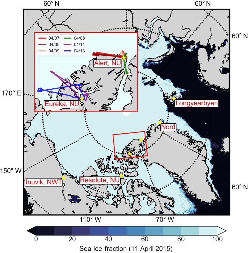
2 Methods Figure 1. Map of the NETCARE 2015 campaign study area, show-
ing sea ice concentrations on 11 April 2015 (Spreen et al., 2008). All
2.1 High Arctic measurements stations along the NETCARE/PAMARCMiP 2015 track are shown
with yellow stars (Longyearbyen, Svalbard; Alert, Nunavut; Eu-
2.1.1 Measurement platform and inlets reka, Nunavut; Resolute Bay, Nunavut; and Inuvik, Northwest Ter-
ritories). Parallels are shown in dashed circles at 60, 70 and 80◦ N.
Measurements of aerosol, trace gases and meteorological pa- Inset: flight tracks from six flights during 7–13 April 2015 based in
rameters were made in High Arctic spring aboard the Al- Alert and Eureka, Nunavut, which are the focus of this work.
fred Wegener Institute (AWI) Polar 6 aircraft, an unpres-
surized DC-3 aircraft converted to a Basler BT-67 (Herber
et al., 2008), as part of the Network on Climate and Aerosols: let, with near-unity transmission of particles 20 nm to ∼ 1 µm
Addressing Key Uncertainties in Remote Canadian Envi- in diameter at typical survey airspeeds and a total flow rate
ronments project (NETCARE, http://www.netcare-project. of approximately 55 L min−1 . Bypass lines off the main in-
ca, last access: 20 December 2018), and in partnership let, at angles of 45◦ , carried aerosol to various instruments.
with the Polar Airborne Measurements and Arctic Regional Performance of the aerosol inlet used here was characterized
Climate Model Simulation Project (PAMARCMiP; Herber by Leaitch et al. (2016). Aerosol was not actively dried prior
et al., 2012). Measurements on a total of 10 flights took to sampling; however, the temperature in the inlet line within
place from 4 to 22 April 2015, based at four stations along the aircraft cabin was at least 15 ◦ C warmer than the ambi-
the PAMARCMiP track: Longyearbyen, Svalbard (78.2 ◦ N, ent temperature so that the relative humidity (RH) decreased
15.6 ◦ E); Alert, Nunavut, Canada (82.5 ◦ N, 62.3 ◦ W); Eu- significantly.
reka, Nunavut, Canada (80.0 ◦ N, 85.9 ◦ W); and Inuvik,
Northwest Territories, Canada (68.4 ◦ N, 133.7 ◦ W). To fo- 2.1.2 State parameters
cus our analysis on aerosol within the polar dome, a sub-
set of six flights in the High Arctic during 7–13 April 2015 State parameters and meteorological conditions were mea-
are considered in this analysis (Fig. 1). The vertical extent sured with an AIMMS-20, manufactured by Aventech
of these flights is shown in Fig. S1 in the Supplement. Dur- Research Inc. (Barrie, ON, Canada; https://aventech.com/
ing measurement flights aircraft speed was maintained at products/aimms20.html, last access: 20 December 2018).
∼ 75 m s−1 (∼ 270 km h−1 ), with ascent and descent rates of The AIMMS-20 consists of three modules: (1) an Air
∼ 150 m min−1 . Data Probe, which measures temperature and the three-
Aerosol and trace gas inlets were identical to those used dimensional aircraft-relative flow vector (total air speed TAS,
aboard Polar 6 during the NETCARE 2014 summer cam- angle of attack, and side slip) with a three-dimensional ac-
paign and are described in Leaitch et al. (2016) and Willis celerometer for measurement of turbulence; (2) an Inertial
et al. (2016). Briefly, aerosol was sampled approximately Measurement Unit, which provides the aircraft angular rate
isokinetically through a stainless steel shrouded diffuser in- and acceleration; and (3) a Global Positioning System for
Atmos. Chem. Phys., 19, 57–76, 2019 www.atmos-chem-phys.net/19/57/2019/
M. D. Willis et al.: Spring Arctic aerosol                                                                                    61

aircraft three-dimensional position and inertial velocity. Ver-    tions (Brock et al., 2011; Kupc et al., 2018). However, com-
tical and horizontal wind speeds are measured with accura-         parison between particle measurements during NETCARE
cies of 0.75 and 0.50 m s−1 respectively. Accuracy and pre-        2015 suggests that these effects are not significant, likely
cision of the temperature measurement are 0.30 and 0.10 ◦ C        owing to the relatively slow vertical speed of the Polar 6
respectively. Potential temperature was calculated using tem-      (Schulz et al., 2018). Owing to these instrumental discrepan-
perature and pressure measured by the AIMMS-20.                    cies present at low particle number concentrations, we em-
                                                                   phasize that absolute particle number concentrations should
2.1.3   Trace gases                                                be treated with caution.

Carbon monoxide. CO concentrations were measured at                2.1.5   Particle composition
1 Hz with an Aerolaser ultra-fast carbon monoxide monitor
(model AL 5002), based on VUV fluorimetry using excita-            Refractory black carbon. Concentrations of particles con-
tion of CO at 150 nm. The instrument was modified such that        taining refractory black carbon (rBC) were measured with a
in situ calibrations could be conducted in flight. Measured        DMT single-particle soot photometer (SP2) (Schwarz et al.,
concentrations were significantly higher than the instrument       2006; Gao et al., 2007). The SP2 uses a continuous intra-
detection limit. The measurement precision is ±1.5 ppbv ,          cavity Nd:YAG laser (1064 nm) to classify particles as either
with an instrument stability based on in-flight calibrations of    incandescent (rBC) or scattering (non-rBC), based on the in-
1.7 %.                                                             dividual particle’s interaction with the laser beam. The peak
   Water vapour and carbon dioxide. H2 O and CO2 measure-          incandescence signal is linearly related to the rBC mass. The
ments were made at 1 Hz using non-dispersive infrared ab-          SP2 was calibrated with Fullerene Soot (Alfa Aesar) stan-
sorption with a LI-7200 enclosed CO2 /H2 O analyzer from           dard by selecting a narrow size distribution of particles with
LI-COR Biosciences. In situ calibrations were performed            a differential mobility analyzer upstream of the SP2 (Laborde
during flight at regular intervals (15–30 min) using a NIST        et al., 2012). The SP2 efficiently detected particles with rBC
traceable CO2 standard with zero water vapour concentra-           mass of 0.6 to 328.8 fg, which corresponds to 85–704 nm
tion. Measured concentrations were significantly higher than       mass equivalent diameter (assuming a void free bulk mate-
the instrument detection limit. The measurement precision          rial density of 1.8 g cm−3 ). rBC mass concentrations were
for CO2 is ±0.05 ppmv , with an instrument stability based         not corrected for particles outside the instrument size range,
on in-flight calibrations of 0.5 %. The measurement precision      and the measurement uncertainty is ±15 % (Laborde et al.,
for H2 O is ±18.5 ppmv , with an instrument stability based on     2012). Measurements of rBC during NETCARE 2015 are
in-flight calibrations of 2.5 %.                                   discussed in detail by Schulz et al. (2018).
   Ozone. O3 concentrations were measured, with a time                Non-refractory aerosol composition. Non-refractory
resolution of 10 s, using UV absorption at 254 nm with a           aerosol composition was measured with an Aerodyne time-
Thermo Scientific ozone analyzer (model 49i). The measure-         of-flight aerosol mass spectrometer (ToF-MS) (DeCarlo
ment uncertainty is ±0.2 ppbv .                                    et al., 2006). Operation of the ToF-AMS aboard Polar 6
                                                                   and characterization of the pressure-controlled inlet system
2.1.4   Particle concentrations                                    is described in Willis et al. (2016, 2017). The ToF-AMS
                                                                   deployed here was equipped with an infrared laser vapor-
Aerosol number size distributions from 100 nm to 1 µ m were        ization module similar to that of the DMT SP2 (SP laser)
acquired with two instruments: (1) a Droplet Measurement           (Onasch et al., 2012); however, rBC concentrations during
Technology (DMT) Ultra-High Sensitivity Aerosol Spec-              the flights discussed here were generally below ToF-AMS
trometer (UHSAS) with a flow rate of 55 cm3 min−1 from             detection limits (∼ 0.1 µg m−3 for rBC) so SP2 measure-
a bypass flow off the main aerosol inlet, and (2) a GRIMM          ments of rBC are used in this work. The instrument was
sky optical particle counter (Sky-OPC, model 1.129) with           operated up to an altitude of ∼ 3.5 km, and the temperature
a flow rate of 1200 cm3 min−1 from a bypass flow off the           of the ToF-AMS was passively maintained using a modular
main aerosol inlet (Cai et al., 2008). In their overlapping size   foil-lined insulating cover. The ToF-AMS was operated
range, comparison of UHSAS and OPC particle number con-            in “V-mode” with a mass range of m/z 3–290, alternating
centrations suggested that the UHSAS underestimated the            between ensemble mass spectrum (MS) mode for 10 s (two
concentration of larger particles (> 500 nm). This compari-        cycles of 5 s MS open and 5 s MS closed) with the SP laser
son is presented in Fig. S2 and discussed further in Supple-       on, MS mode with the SP laser off for 10 s, and efficient
ment Sect. S1. We therefore present these observations as          particle time-of-flight (epToF) mode with the SP laser on for
the number of particles between 100 and 500 nm (N100–500 )         10 s (Supplement Table S1) (DeCarlo et al., 2006; Onasch
derived from UHSAS observations and the number greater             et al., 2012). Single-particle observations were made on two
than 500 nm (N>500 ) from the OPC. Recent work has high-           flights; this ToF-AMS operation mode is described below.
lighted the impact of rapid pressure changes, during aircraft      Only observations made with the SP laser off are used
ascent and descent, on reported UHSAS particle concentra-          to quantify non-refractory aerosol composition. Filtered

www.atmos-chem-phys.net/19/57/2019/                                                     Atmos. Chem. Phys., 19, 57–76, 2019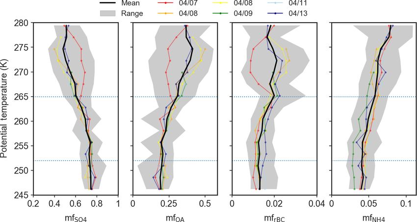
62                                                                                  M. D. Willis et al.: Spring Arctic aerosol

ambient air was sampled with the ToF-AMS at least 3 times            ToF-AMS total non-refractory aerosol mass correlated
per flight, for a duration of at least 5 min, to account for      well with estimated aerosol mass from the UHSAS and OPC,
contributions from air signals.                                   but was generally higher by approximately a factor of 2
   Species comprising non-refractory particulate matter           (Fig. S4, assuming a mean density of 1.5 g cm−3 ). An im-
are quantified by the ToF-AMS, including sulfate (SO4),           portant exception to this observation occurred when the ToF-
nitrate (NO3), ammonium (NH4), and the sum of organic             AMS measured significant NaCl+ ; at these times, the ToF-
species (OA). The ToF-AMS is also capable of detecting sea        AMS total aerosol mass was relatively constant while the es-
salt (Ovadnevaite et al., 2012). The detection efficiency of      timated mass increased, indicating that sea salt was an im-
sea-salt-containing particles is dependent on not only the        portant contributor to aerosol mass. These discrepancies are
ambient RH but also the temperature of the tungsten vapor-        discussed further in Sect. S1 of the Supplement. Owing to
izer (Ovadnevaite et al., 2012). A quantitative estimate of sea   the discrepancies between measured and estimated particle
salt mass is not possible with these measurements and this        mass, we emphasize that absolute mass concentrations pre-
species is not included in the calculation of aerosol chemical    sented in this work should be treated with caution; however,
mass fractions, such that the mass fractions presented            these discrepancies do not prevent a useful interpretation of
represent non-refractory aerosol species and rBC measured         the ToF-AMS data based upon relative changes in particle
by the SP2. The vaporizer temperature was calibrated with         composition.
sodium nitrate particles and was operated at a temperature of        ToF-AMS single-particle measurements. The ToF-AMS
∼ 650 ◦ C. ToF-AMS signals for sea salt, in particular NaCl+      was operated in Event Trigger Single Particle (ETSP) mode
(m/z 57.96), can be used to quantify sea salt (Ovadnevaite        on two flights (Table S1). ETSP is run in the single-slit
et al., 2012); however, here we use the NaCl+ signal only         particle-time-of-flight (pToF) mode. A particle event is de-
as a qualitative indication for the presence of sea salt          fined as a single mass spectrum (MS) extraction or set of
owing to uncertainties in sea salt collection efficiency as       consecutive MS extractions associated with a single parti-
a function of RH and the lack of RH measurement in the            cle being vaporized and producing MS signals. The number
sampling line. Ammonium nitrate calibrations (Jimenez             of MS extractions obtained during a particle event is deter-
et al., 2003) were carried out twice during the campaign          mined by the pulser frequency, and thus the mass range, set
as well as before and after, owing to restricted access to        during acquisition; in this case 30.9 kHz, corresponding to
calibration instruments during the campaign. Air-beam             a pulser period of 32.4 µs (m/z 3–290). Under these condi-
corrections were referenced to the appropriate calibration        tions, at least a single mass spectrum is collected per particle
in order to account for differences in instrument sensitivity     event. Saving mass spectra associated with a particle event
between flights. The relative ionization efficiencies for         is triggered in real time based on the signals present in up to
sulfate and ammonium (RIESO4 and RIENH4 ) were 0.9 ± 0.1          three continuous ranges of mass-to-charge ratios, called re-
and 3.4 ± 0.3. The default relative ionization efficiency         gions of interest (ROIs). Three ROIs were used in this work
for organic species (i.e., RIEOrg = 1.4) was used, which is       such that a signal above a specified ion threshold in any ROI
appropriate for oxygenated organic aerosol (Jimenez et al.,       would trigger saving a mass spectrum (Table S2). Ion thresh-
2003, 2016). Elemental composition was calculated using           olds were purposely set low to collect a large number of false
the method presented in Canagaratna et al. (2015). Data           positives that are subsequently removed based on the rela-
were analyzed using the Igor Pro-based analysis tool PIKA         tionship between total aerosol ion signal (i.e., excluding air)
(v.1.16H) and SQUIRREL (v.1.57l) (DeCarlo et al., 2006;           and particle size (Fig. S5), similar to the approach described
Sueper, 2010). Detection limits and propagated uncertainties      in Lee et al. (2015). Two background regions in the particle
(i.e., ±(detection limit + total uncertainty)) for sulfate,       size distribution (10–50 and 2000–4000 nm) were selected
nitrate, ammonium, and organics at a 10 s time resolution         to determine the average background ion signal excluding
were ±(0.009 µg m−3 + 35 %), ±(0.001 µg m−3 + 33 %),              air peaks, and particle events considered “real” must be be-
±(0.003 µg m−3 + 33 %), and ±(0.08 µg m−3 + 37 %),                tween 80 and 1000 nm with ion signals above the mean back-
respectively. We note that ion ratios commonly reported           ground plus 3 times its standard deviation (Fig. S5). A sim-
from ToF-AMS measurements of ammonium and sulfate                 plified fragmentation table, described in Lee et al. (2015),
are not appropriate for estimating aerosol neutralization         was applied to particle mass spectra identified as “real” and
(Hennigan et al., 2015), so we do not report these here. A        fragmentation corrections were based on higher mass res-
composition-dependent collection efficiency (CDCE) was            olution ensemble MS spectra collected concurrently. A to-
applied to correct ToF-AMS mass loadings for non-unity            tal of 1677 “real” particle spectra were collected over two
particle detection due to particle bounce on the tungsten         flights (8 and 13 April 2015). A k-means cluster analysis
vaporizer (Middlebrook et al., 2012), which resulted in           was applied to particle spectra to explore different particle
a median (quartile range) collection efficiency correction        mixing states, following Lee et al. (2015). A two-cluster so-
of 18 % (12 %–28 %) applied uniformly to non-refractory           lution was selected to describe the 1677 total “real” parti-
aerosol species.                                                  cle spectra. Owing to the small number of particle spectra
                                                                  and the lack of specificity in organic aerosol peaks from

Atmos. Chem. Phys., 19, 57–76, 2019                                                   www.atmos-chem-phys.net/19/57/2019/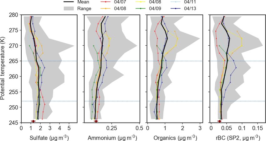
M. D. Willis et al.: Spring Arctic aerosol 63
highly oxygenated aerosol, increasing the number of clus- and space), with constraints on altitude and location. This
ters did not yield physically meaningful information. Mean residence time is reported as a relative residence time over
mass spectra and mass spectral histograms for each particle the 10-day FLEXPART-ECMWF backward integration time.
class are shown in Fig. S6. ETSP data were analyzed using Aircraft observations were sub-sampled to the model time
the Igor Pro-based analysis tools Tofware version 2.5.3.b (de- resolution by taking a 1 min average of measurements around
veloped by TOFWERK and Aerodyne Research, Inc.), clus- the model release time, when the aircraft altitude was within
tering input preparation panel (CIPP) version ETv2.1b and ±100 m of the model release altitude.
cluster analysis panel (CAP) version ETv2.1 (developed by
Alex K. Y. Lee and Megan D. Willis).
3 Results and discussion
2.2 Air mass history from particle dispersion modelling
3.1 Transport regimes in the polar dome
The Lagrangian particle dispersion model FLEXible PARTi-
cle (FLEXPART) (Brioude et al., 2013) driven by meteoro- We focus on observations made on six flights in the High
logical analysis data from the European Centre for Medium- Arctic during NETCARE 2015 over the period 7–13 April
Range Weather Forecasts (ECMWF) was used to study the 2015. Figure 1 illustrates flight tracks during this period on
history of air masses prior to sampling during NETCARE a map of the sea ice concentration from 11 April 2015. Ob-
flights. The ECMWF data had a horizontal grid spacing of servations of trace gas gradients during this campaign de-
0.25◦ and 137 vertical levels. Here, we use FLEXPART- fined the region inside the polar dome as north of 69◦ 300 N
ECMWF run in backward mode to study the origin of air and below 280.5 K (∼ 3.5 km) (Bozem et al., 2018). Zonal
influencing aircraft-based aerosol and trace gas measure- mean potential temperature cross sections from ECMWF for
ments. Individual FLEXPART parcels were initialized along the period 7–13 April 2015 generally agree with this defini-
the flight track every 3 min and then traced back in time tion of the polar dome, and this demonstrates that our ob-
for 10 days, providing time-resolved information on source servations were made in the coldest air masses present in
regions of trace species measured along the flight track. the Arctic region during this time (Fig. S7). CO concentra-
FLEXPART-ECMWF output was provided every 3 h over tions observed in the polar dome were consistent with “Arctic
the 10-day period, with horizontal grid spacing of 0.25◦ and background” air masses identified in previous airborne obser-
10 vertical levels (50, 100, 200, 500, 1000, 2000, 4000, 6000, vations and with monthly mean CO concentrations at Alert,
8000 and 10 000 m). In backward mode, the model provides Nunavut, Canada (Fig. S8). This suggests that our observa-
an emission sensitivity function called the potential emission tions during April 2015 in the polar dome were not strongly
sensitivity (PES). The PES in a particular grid cell, or air impacted by episodic transport events of high pollutant con-
volume, is the response function of a source–receptor rela- centrations (Brock et al., 2011). We restrict our analysis to
tionship, and is proportional to the particle residence time in those air masses residing in the polar dome, to determine the
that grid cell (e.g., Hirdman et al., 2010). PES values can be sources and processes contributing to aerosol composition
combined with emission distributions to calculate receptor within this region during spring. When discussing observa-
concentrations, assuming the species is inert; however, we tions and model predictions, we use potential temperature in-
use the PES directly and show maps of PES with units of stead of height or pressure for two reasons. First, the location
seconds (i.e., proportional to air mass residence time). Ab- of the polar dome and transport northward are dictated by po-
solute residence times depend on the model output time step tential temperature rather than absolute height. Second, trace
and the extent of spatial averaging. Maps of PES represent gases and aerosol observed in the polar dome varied system-
integration of model output over a period of time prior to atically with potential temperature, but showed less system-
sampling (i.e., 10 days), also referred to as the “time before atic variability with pressure (Fig. S9). Altitude profiles of
measurement”, and over a vertical range. We show maps of absolute and potential temperature are shown in Fig. S10. In
both the total column PES (i.e., 0–20 km) and partial column this section, we discuss transport patterns inferred from trace
PES (i.e., 0–200 m), as emissions near the surface are of par- gas observations and FLEXPART-ECMWF air mass history,
ticular interest. and in Sect. 3.2 we discuss observed aerosol composition in
By integrating model output at each model release over the context of these transport patterns.
specific pressure levels and/or latitude ranges we used Trends in trace gas concentrations with potential temper-
FLEXPART-ECMWF to calculate the residence time of air ature illustrate different transport regimes within the polar
in the middle-to-lower polar dome. The horizontal extent of dome (Fig. 2). Based on the mean vertical profiles of trace
the polar dome was defined based on Bozem et al. (2018) gases, we divided observed vertical profiles into three ranges
as north of 69◦ 300 N. The vertical extent of the middle-to- of potential temperature (Fig. 2: 245–252, 252–265 and 265–
lower polar dome was defined based on trace gas profiles 280 K) to guide interpretation of air mass history, transport
as below 265 K (∼ 1550 m). Calculation of this quantity is characteristics and aerosol composition in the polar dome.
analogous to calculating the PES (i.e., by integrating in time We refer to these three ranges of potential temperature as the
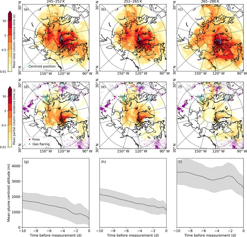
www.atmos-chem-phys.net/19/57/2019/ Atmos. Chem. Phys., 19, 57–76, 201964 M. D. Willis et al.: Spring Arctic aerosol Figure 2. Mean potential temperature profiles of trace gases (CO, CO2 , O3 and H2 O) and particle concentrations (N100–500 and N>500 ) in the polar dome observed during 7–13 April 2015. Coloured lines indicate the mean profile for each flight, the black line represents the mean profile over all flights, and gray shading shows the range of observations in each potential temperature bin. Horizontal dashed blue lines separate the lower, middle and upper polar dome defined as 245–252, 252–265 and 265–280 K. lower, middle and upper polar dome, respectively (dashed lar dome, while N100–500 showed more variability compared horizontal lines in Fig. 2), and discuss the characteristics to colder potential temperatures. of each region in turn. First, in the coldest and driest air The importance of lower latitude source regions increases masses (245–252 K), we consistently observed temperature as potential temperature increases in the polar dome. The dis- inversion conditions, with potential temperature increasing tribution of FLEXPART-ECMWF potential emission sensi- by 37 K km−1 compared to 11 K km−1 above the lower polar tivities (Fig. 3) indicates that most air masses in the lower and dome (Fig. S10). Temperature inversions are frequent in the middle polar dome had resided there for at least 10 days, with High Arctic spring, with median inversion strengths of ∼ 5– significant sensitivity to the surface north of 80◦ N and some 10 K occurring frequently in March, April and May (Bradley sensitivity to high-latitude Eurasia. The fraction of the previ- et al., 1992; Tjernström and Graversen, 2009; Zhang et al., ous 10 days spent in the polar dome is highest in the middle 2011; Devasthale et al., 2016). Owing to the static stability and lower polar dome, while above ∼ 265 K this quantity de- of the lower polar dome under these conditions, these air creases significantly (Fig. 4, S8). This observation indicates masses may be isolated from the air aloft and may be sen- a clear separation in air mass history between the middle-to- sitive to different sources and transport history (Stohl, 2006). lower polar dome and the upper polar dome. Sensitivity to Under these stable conditions, CO and CO2 were relatively lower latitude regions increases as potential temperature in- constant (mean (quartile range), 144.5 (144.2–146.5) ppbv creases in the polar dome, particularly in high-latitude Eura- and 405.8 (405.4–406.2) ppmv , respectively) in the lower po- sia and North America (Fig. 3). Locations of active fires lar dome and O3 was depleted to 11.4 (3.1–23.4) ppbv . Ac- during 28 March 2015–13 April 2015 and of oil and gas tive halogen production and resulting O3 depletion may oc- extraction emissions (Fig. 3) indicate that biomass burning cur largely at the surface (e.g., Spackman et al., 2010; Olt- emissions likely had a stronger influence on the upper polar mans et al., 2012; Abbatt et al., 2012; Pratt et al., 2013). dome, while oil and gas extraction emissions may be more It follows that the observed O3 profile could be interpreted important in the lower polar dome. Total March–May 2015 as an indication of mixing of O3 -depleted air from the sur- fire counts in the Northern Hemisphere were comparable to face up to ∼ 252 K (∼ 400 m). Particle number concentra- previous years (Fig. S12), but were significantly lower than tions between 100 and 500 nm (N100–500 ) were relatively 2008. This suggests that biomass burning sources are often constant in the lower polar dome (∼ 150 cm−3 ), while larger less important sources of Arctic aerosol than has been sug- accumulation mode particles (N>500 ) were most abundant in gested by previous observations from the year 2008 (e.g., the lower polar dome compared to higher potential tempera- Warneke et al., 2009; Brock et al., 2011; Hecobian et al., tures (∼ 4 cm−3 compared to < 1 cm−3 ). Second, in the mid- 2011; McNaughton et al., 2011; Liu et al., 2015). dle polar dome (252–265 K), O3 increased toward ∼ 50 ppbv A prevalent feature of air mass histories in the lower and and CO and CO2 remained relatively constant while water middle polar dome is descent from aloft over at least 10 days vapour showed more variability. Finally, at the highest poten- prior to our measurements (Fig. 3g, h). The FLEXPART- tial temperatures we observed more variability in CO, CO2 ECMWF-predicted plume centroid also shows some evi- and H2 O, while O3 concentrations were relatively constant at dence for descent in the upper polar dome (Fig. 3i), though 49.6 (45.7–54.1) ppbv . N>500 was near zero in the upper po- we note that descent from aloft in the plume centroid does not Atmos. Chem. Phys., 19, 57–76, 2019 www.atmos-chem-phys.net/19/57/2019/
M. D. Willis et al.: Spring Arctic aerosol                                                                                                65

Figure 3. FLEXPART-ECMWF potential emission sensitivity (PES) and plume centroid altitude averaged over three potential temperature
ranges in the polar dome. (a–c) Mean total column PES, (d–f) mean partial column (< 200 m) PES, (g–i) mean plume centroid altitudes for
245–252 K (a, d, g), 252–265 K (b, e, h) and 265–280 K (c, f, i). Fire locations during 28 March to 13 April 2015 from MODIS are purple
points, gas flaring locations associated with oil and gas extraction from the ECLIPSE emission inventory (V5) for 2015 are light blue points.
Parallels are shown in dashed circles at 45, 60 and 80◦ N.

preclude some sensitivity to the surface. Air mass descent in            into the polar dome (Stohl, 2006). In the next section, we
the polar dome is likely caused by a combination of both ra-             discuss observed aerosol composition in the context of these
diative cooling (on the order of 1 K day−1 ; Klonecki et al.,            transport patterns.
2003) and orographic effects over nearby elevated terrain on
Ellesmere Island and Greenland. With long aerosol lifetimes              3.2   Aerosol composition in the polar dome
under cold and relatively dry conditions in the polar dome,
this suggests that aerosol in the upper polar dome can influ-
                                                                         Vertical variability in aerosol composition was systematic
ence the lower and middle polar dome on the timescale of
                                                                         across flights in the polar dome during April 2015. Sub-
10 days and longer. Transport times to the Arctic lower tro-
                                                                         micron aerosol present in the coldest air masses of the lower
posphere are likely longer than 10 days (e.g., Brock et al.,
                                                                         polar dome contained the highest fraction of sulfate (74 %
2011; Qi et al., 2017; Leaitch et al., 2018), suggesting that
                                                                         by mass, Fig. 5). This trend in the sulfate mass fraction
a major springtime transport mechanism may be lofting near
                                                                         (mfSO4 ) was driven by both decreasing sulfate and increas-
source regions, followed by northward transport and descent
                                                                         ing organic aerosol concentrations as potential temperature

www.atmos-chem-phys.net/19/57/2019/                                                              Atmos. Chem. Phys., 19, 57–76, 2019
66 M. D. Willis et al.: Spring Arctic aerosol
Figure 5. Mean potential temperature profiles of relative aerosol
Figure 4. Observed potential temperature (K) versus FLEXPART- composition, including mass fractions of sulfate (mfSO4 ), organic
ECMWF-predicted fraction of the past 10 days in the polar dome aerosol (mfOA ), refractory black carbon (mfrBC ), and ammonium
(i.e., below 280.5 K and north of 69◦ 300 N). The FLEXPART- (mfNH4 ), in the polar dome observed during 7–13 April 2015.
ECMWF relative residence time is binned in the lower (245–252 K), Coloured lines indicate the mean profile for each flight, the black
middle (252–265 K) and upper (265–280 K) polar dome. line represents the mean profile over all six flights, and gray shad-
ing shows the range of observations in each potential temperature
bin.
increased (Figs. 6, S5). This observation is broadly consistent
with previous vertically resolved measurements of aerosol
sulfate in both the Canadian Arctic and Alaskan Arctic dur-
ing spring that have indicated increasing sulfate concentra-
tions toward lower altitudes (Scheuer et al., 2003; Bour-
geois and Bey, 2011). Large contributions of sulfate to near-
surface Arctic spring aerosol is also consistent with ground-
based observations at long-term monitoring stations includ-
ing Zeppelin, Svalbard; Alert, Nunavut; and Utqiaġvik (Bar-
row), Alaska (e.g., Barrie and Hoff, 1985; Quinn et al., 2007;
Breider et al., 2017; Leaitch et al., 2018). The mass frac-
tion of ammonium (mfNH4 ) increases with increasing poten-
tial temperature. This trend is driven by both decreasing sul- Figure 6. Mean potential temperature profiles of absolute (STP)
fate concentration and increasing ammonium concentration sub-micron aerosol composition in the polar dome observed during
as potential temperature increases (Fig. 6). This observation 7–13 April 2015, including sulfate, organics and ammonium from
is broadly consistent with previous vertically resolved mea- the ToF-AMS and refractory black carbon (rBC) from the SP2. Ni-
surements in the North American Arctic from April 2008 trate concentrations were negligible, and largely below detection
limits. Coloured lines indicate the mean profile for each flight, the
that demonstrated increased ammonium relative to sulfate to-
black line represents the mean profile over all six flights, and gray
ward higher altitudes (Fisher et al., 2011). However, Fisher shading shows the range of observations in each potential tempera-
et al. (2011) observed significantly higher ammonium rela- ture bin. Single points at the lowest potential temperature represent
tive to sulfate compared to our measurements. These differ- concentrations of sulfate, ammonium and rBC measured at Alert,
ences may arise from the larger altitude range in Fisher et al. NU, during 6–13 April 2015 from Macdonald et al. (2017). Points
(2011) (up to ∼ 10 km) and differences in source regions or represent the mean concentration and error bars represent measure-
source strengths between 2008 and 2015. ment uncertainty.
Organic aerosol and refractory black carbon were more
abundant in the upper polar dome, while sulfate was less
abundant. On average, OA and rBC contributed 42 % and unique mass spectral fragments from this highly oxygenated
2 % to aerosol mass, respectively, in the upper polar dome. OA, our ToF-AMS spectra cannot distinguish differences in
OA was highly oxygenated throughout the polar dome, with OA composition in the polar dome. Overall, our observations
oxygen-to-carbon (O / C) ratios above 0.5 in the majority of suggest that surface-based measurements may underestimate
measurements (Fig. S13). High O / C ratios are consistent the contribution of OA, rBC and ammonium to aerosol trans-
with an abundance of highly functionalized organic acids ob- ported to the Arctic troposphere in spring.
served in Arctic haze aerosol at Alert, Nunavut, during spring Air masses spent the longest times in the middle to lower
(Kawamura et al., 1996, 2005, 2010; Narukawa et al., 2008; polar dome (Fig. 4), and aerosol composition varied system-
Fu et al., 2009; Leaitch et al., 2018). Owing to the lack of atically with time spent in this portion of the polar dome. The
Atmos. Chem. Phys., 19, 57–76, 2019 www.atmos-chem-phys.net/19/57/2019/M. D. Willis et al.: Spring Arctic aerosol 67
mass fractions of OA and rBC decrease with the FLEXPART-
ECMWF-predicted fraction of the previous 10 days spent
north of 69◦ 300 N and below 265 K (Fig. 7). OA and rBC
were well-correlated in the middle and upper polar dome
(Fig. S14), suggesting that these species have a similar source
region and/or have undergone similar processing. A domi-
nance of anthropogenic (fossil fuel) sources of black carbon
to the High Arctic during April 2015 may explain this re-
lationship between rBC and OA. The importance of anthro-
pogenic emissions of black carbon from eastern and south-
ern Asia to measured Arctic black carbon in spring was re-
cently demonstrated using a chemical transport model con-
strained by our measurements of black carbon in combi-
nation with surface sites and previous aircraft-based cam-
paigns (Xu et al., 2017). European and north Asian anthro-
pogenic emissions contributed significantly to Arctic black
carbon in the lowest kilometre, with eastern and southern
Asian sources increasing in importance toward higher alti-
tudes (Xu et al., 2017). Southern Asian regions are not well-
represented in 10-day FLEXPART-ECMWF backward sim-
ulations, which likely do not capture transport back to all
source regions (Qi et al., 2017; Leaitch et al., 2018). OA Figure 7. Sub-micron aerosol mass fractions versus FLEXPART-
and rBC are largely uncorrelated in the lower polar dome, ECMWF-predicted fraction of the previous 10 days prior to
suggesting shifting source regions and/or chemical process- measurement spent in the middle-to-lower polar dome (north of
ing of OA toward lower potential temperatures. This obser- 69◦ 300 N, Bozem et al., 2018, and, based on trace gas profiles,
vation is consistent with multi-year observations from Alert, below 265 K, ∼ 1600 m). Data points corresponding to individual
Nunavut, showing that black carbon and organic matter are FLEXPART-ECMWF releases are shown as circles, and summary
correlated during winter, but become uncorrelated during statistics are shown as boxes (25th, 50th, 75th percentiles) and
whiskers (5th, 95th percentiles) for data binned by time spent in
spring (Leaitch et al., 2018).
the middle and lower polar dome.
In contrast to OA and rBC, the mass fraction of sulfate
increases with increasing time spent in the middle-to-lower
polar dome (Fig. 7). In the upper polar dome the ammonium- be changing as a result of chemical processing over the long
to-sulfate molar ratio is at times consistent with ammonium aerosol lifetime. The fraction of sulfate could be increasing
bisulfate, while more sulfuric acid is likely present at lower with decreasing potential temperature as a result of oxidation
potential temperatures. The enhanced fraction of sulfate in of transported sulfur dioxide and subsequent condensation
the lower polar dome compared to higher potential temper- of sulfuric acid onto existing particles as air masses slowly
atures could arise from a combination of possible mech- descend (Fig. 3). In addition, oxidation of existing OA, re-
anisms. First, the stability of the polar dome may cause sulting in fragmentation and loss of aerosol mass to the gas
systematic vertical variability in source regions throughout phase, could contribute to a decrease in OA concentrations
the polar dome (e.g., Stohl, 2006). The observed middle-to- toward lower altitudes (e.g., Kroll et al., 2009); however, this
lower polar dome aerosol composition could arise from high- process may be less important at low temperatures. Descent
latitude, sulfur-rich emissions in the absence of significant from aloft appears to be an important transport mechanism
ammonia and organic aerosol sources. A complex mixture influencing the lower polar dome in our flight area, lending
of natural and anthropogenic sources has previously been some support to this second set of processes. Finally, wet
shown to contribute to observed variations in sulfate and am- removal or cloud processing of aerosol over long transport
monium with altitude in Arctic spring (Fisher et al., 2011). times likely impacts the aerosol composition we observe,
In the lowest 2 km, emissions from non-Arctic Russia and though we cannot distinguish this influence with our mea-
Kazakhstan (included as part of eastern and southern Asia surements. In the next section, we examine the characteris-
in Xu et al., 2017), along with North American emissions, tics of lower polar dome aerosol in detail and compare it to
were the dominant sources of sulfate in April 2008 (Fisher aerosol present in the middle and upper polar dome.
et al., 2011). At higher altitudes, model results suggested
eastern Asian sources of sulfate became more important and, 3.3 Characteristics of lower polar dome aerosol
along with European sources, were the main contributor of
sulfate aerosol in Arctic spring. Second, and possibly in ad- Lower polar dome air masses had resided for the longest
dition to shifting source regions, aerosol composition could times within the polar dome (Figs. 3, 4 and S11), suggesting
www.atmos-chem-phys.net/19/57/2019/ Atmos. Chem. Phys., 19, 57–76, 201968 M. D. Willis et al.: Spring Arctic aerosol
Figure 8. Potential temperature profiles of the ToF-AMS NaCl+
signal (top axis), as a qualitative indication of the presence of sea
salt aerosol, and N>500 (bottom axis). The solid lines represent the
mean profile for 7–13 April 2015, and shading represents the range
of measurements in each potential temperature bin.
Figure 9. (a) Normalized mean ToF-AMS size distributions of sul-
fate subset by observed potential temperature: below 252 K (black),
that this aerosol likely had a lifetime of 10 days or longer. above 265 K (light blue). (b) ToF-AMS size distributions of sulfate
This aerosol was comprised largely of sulfate, with smaller (red) and total organic aerosol (green) below 252 K. The mass frac-
amounts of OA, rBC and ammonium compared to aerosol tion of sulfate calculated from ToF-AMS size distributions is shown
on the right axis in black circles, and is calculated only between 200
present in the middle and upper polar dome (Sect. 3.2). In ad-
and 600 nm owing to low OA signals at smaller and larger sizes.
dition, ToF-AMS spectra provide qualitative evidence for the Shading corresponds to ±1 standard deviation for sulfate and or-
presence of sea salt aerosol in the lower polar dome, which ganic aerosol size distributions, and the relatively large variation in
decreases to negligible concentrations through the middle size-resolved composition indicates that the derived mass fraction
polar dome (Fig. 8). The ToF-AMS NaCl+ signal and N>500 of sulfate as a function of size is uncertain.
have a similar profile, suggesting that sea salt may be as-
sociated with the increase in larger accumulation mode par-
ticles observed in the lower polar dome. This observation lower polar dome aerosol. Recent observations at Utqiaġvik
is consistent with previous airborne measurements in the (Barrow), Alaska, have demonstrated the prevalence of sea
Alaskan Arctic during spring that showed the largest frac- salt aerosol in Arctic winter and significant mixing with sul-
tion of sea salt particles were present in air masses identified fate (Kirpes et al., 2018). Sulfate may be internally mixed
as associated with the “Arctic boundary layer” (i.e., identi- with sea salt in the lower polar dome; however, owing to low
fied by depleted O3 concentrations) (Brock et al., 2011). Sea particle concentrations we are unable to obtain an NaCl+ sig-
salt contributes significantly to aerosol observed at ground- nal from size-resolved mass spectra.
based long-term monitoring stations (e.g., Quinn et al., 2002; Size-resolved observations of non-refractory aerosol com-
Leaitch et al., 2013; Huang and Jaeglé, 2017; Leaitch et al., position provide evidence for different particle mixing states
2018), and peaks in concentration during winter to early across the size distribution. On average, sulfate was present
spring. Sources of sea salt at high northern latitudes in spring in larger particle sizes in the lower polar dome compared to
include transport of sea salt from northern oceans, production the middle and upper polar dome (Fig. 9). In contrast, OA
of sea salt aerosol from open leads in sea ice (e.g., Leck et al., size distributions were very similar in the lower and upper
2002; Held et al., 2011; May et al., 2016), and production of polar dome (Fig. S15). In the lower polar dome, the frac-
saline aerosol through wind driven processes over ice and tion of sulfate increases with particle size (Fig. 9), implying
snow (Yang et al., 2008; Shaw et al., 2010; Xu et al., 2016; the presence of different particle mixing states, and different
Huang and Jaeglé, 2017). The strong decrease in NaCl+ sig- particle sources or chemical processing in the polar dome.
nal and N>500 above the lower polar dome is suggestive of a Single-particle observations from two flights (Figs. 10, S16)
near-surface source of sea salt in the High Arctic; open leads are consistent with these bulk size-resolved observations.
or wind-driven ice and snow processes may contribute to Accumulation mode particles were highly internally mixed,
Atmos. Chem. Phys., 19, 57–76, 2019 www.atmos-chem-phys.net/19/57/2019/You can also read