Evaluation of Southern Ocean cloud in the HadGEM3 general circulation model and MERRA-2 reanalysis using ship-based observations - Recent
←
→
Page content transcription
If your browser does not render page correctly, please read the page content below
Atmos. Chem. Phys., 20, 6607–6630, 2020
https://doi.org/10.5194/acp-20-6607-2020
© Author(s) 2020. This work is distributed under
the Creative Commons Attribution 4.0 License.

Evaluation of Southern Ocean cloud in the HadGEM3
general circulation model and MERRA-2 reanalysis
using ship-based observations
Peter Kuma1 , Adrian J. McDonald1 , Olaf Morgenstern2 , Simon P. Alexander3 , John J. Cassano4,5 , Sally Garrett6 ,
Jamie Halla6 , Sean Hartery1 , Mike J. Harvey2 , Simon Parsons1 , Graeme Plank1 , Vidya Varma2 , and Jonny Williams2
1 School of Physical and Chemical Sciences, University of Canterbury, Christchurch, New Zealand
2 National Institute of Water and Atmospheric Research, Wellington, New Zealand
3 Australian Antarctic Division, Kingston, Australia
4 Cooperative Institute for Research in Environmental Sciences, University of Colorado, Boulder, Colorado, USA
5 Department of Atmospheric and Oceanic Sciences, University of Colorado, Boulder, Colorado, USA
6 New Zealand Defence Force, Wellington, New Zealand

Correspondence: Peter Kuma (peter@peterkuma.net)

Received: 1 March 2019 – Discussion started: 5 April 2019
Revised: 23 April 2020 – Accepted: 28 April 2020 – Published: 5 June 2020

Abstract. Southern Ocean (SO) shortwave (SW) radiation         lator, we find that GA7.1 and MERRA-2 both underestimate
biases are a common problem in contemporary general cir-       low cloud and fog occurrence relative to the ship observa-
culation models (GCMs), with most models exhibiting a ten-     tions on average by 4 %–9 % (GA7.1) and 18 % (MERRA-2).
dency to absorb too much incoming SW radiation. These bi-      Based on radiosonde observations, we also find the low cloud
ases have been attributed to deficiencies in the representa-   to be strongly linked to boundary layer atmospheric stabil-
tion of clouds during the austral summer months, either due    ity and the sea surface temperature. GA7.1 and MERRA-2
to cloud cover or cloud albedo being too low. The problem      do not represent the observed relationship between boundary
has been the focus of many studies, most of which utilised     layer stability and clouds well. We find that MERRA-2 has
satellite datasets for model evaluation. We use multi-year     a much greater proportion of cloud liquid water in the SO in
ship-based observations and the CERES spaceborne radia-        austral summer than GA7.1, a likely key contributor to the
tion budget measurements to contrast cloud representation      difference in the SW radiation bias. Our results suggest that
and SW radiation in the atmospheric component Global At-       subgrid-scale processes (cloud and boundary layer parame-
mosphere (GA) version 7.1 of the HadGEM3 GCM and the           terisations) are responsible for the bias and that in GA7.1
MERRA-2 reanalysis. We find that the prevailing bias is neg-   a major part of the SW radiation bias can be explained by
ative in GA7.1 and positive in MERRA-2. GA7.1 performs         cloud cover underestimation, relative to underestimation of
better than MERRA-2 in terms of absolute SW bias. Sig-         cloud albedo.
nificant errors of up to 21 W m−2 (GA7.1) and 39 W m−2
(MERRA-2) are present in both models in the austral sum-
mer. Using ship-based ceilometer observations, we find low
cloud below 2 km to be predominant in the Ross Sea and         1   Introduction
the Indian Ocean sectors of the SO. Utilising a novel sur-
face lidar simulator developed for this study, derived from    Clouds are considered one of the largest sources of uncer-
an existing Cloud Feedback Model Intercomparison Project       tainty in estimating global climate sensitivity (Boucher et al.,
(CFMIP) Observation Simulator Package (COSP) – active          2013; Flato et al., 2014; Bony et al., 2015). Clouds over
remote sensing simulator (ACTSIM) spaceborne lidar simu-       oceans are especially important for determining the radia-
                                                               tion budget due to the low albedo of the sea surface com-

Published by Copernicus Publications on behalf of the European Geosciences Union.
6608         P. Kuma et al.: Evaluation of Southern Ocean cloud in HadGEM3 and MERRA-2 using ship observations

pared to land. Over the Southern Ocean (SO), cloud cover         ing CBH statistically from CALIPSO measurements (Mül-
is very high at over 80 %, with boundary layer clouds be-        menstädt et al., 2018). Ship-based measurements therefore
ing particularly common (Mace et al., 2009). Excess down-        provide valuable extra information.
ward shortwave (SW) radiation in general circulation mod-           Multiple explanations of the SW radiation bias have been
els (GCMs), with a bias over the SO of up to 30 W m−2 , is       proposed: cloud underestimation in the cold sectors of cy-
a problem documented well by Trenberth and Fasullo (2010)        clones (Bodas-Salcedo et al., 2014), cloud–aerosol interac-
and Hyder et al. (2018) and has been the subject of many         tion (Vergara-Temprado et al., 2018), cloud homogeneity
studies. Bodas-Salcedo et al. (2014) evaluated the SW bias       representation (Loveridge and Davies, 2019), lack of super-
in a number of GCMs and found that a strong SW bias is a         cooled liquid (cloud liquid at air temperature below 0 ◦ C)
very common feature, leading to increased sea surface tem-       (Kay et al., 2016; Bodas-Salcedo et al., 2016) and the “too
perature (SST) in the SO and corresponding biases in the         few, too bright” problem (Nam et al., 2012; Klein et al., 2013;
storm track position. Trenberth and Fasullo (2010) note that     Wall et al., 2017). Each model can exhibit the bias for a dif-
a poor representation of clouds might lead to unrealistic cli-   ferent set of reasons, and results from one model evaluation
mate change projections in the Southern Hemisphere. The          therefore do not necessarily explain biases in all other models
SW bias has also been linked to large-scale model problems,      (Mason et al., 2015). The use of SO voyage data for atmo-
such as the double Intertropical Convergence Zone (Hwang         spheric model evaluation is not new, and has recently been
and Frierson, 2013), biases in the position of the midlatitude   used by Sato et al. (2018) to evaluate the impact of SO ra-
jet (Ceppi et al., 2012) and errors in the meridional energy     diosonde observations on the accuracy of weather forecasting
transport (Mason et al., 2014). Bodas-Salcedo et al. (2012)      models. Klekociuk et al. (2019) contrasted SO cloud obser-
studied the SO SW bias in the context of the Global Atmo-        vations with the ECMWF Interim reanalysis (ERA-Interim)
sphere (GA) 2.0 and 3.0 models and found that mid-topped         and the Antarctic Mesoscale Prediction System–Weather Re-
and stratocumulus clouds are the dominant contributors to        search and Forecasting Model (AMPS-WRF) (Powers et al.,
the bias.                                                        2012) and found that these models underestimate the cover-
   Due to its extent and magnitude, the SW radiation bias is     age of the predominantly low cloud. Protat et al. (2017) com-
believed to limit accuracy of the models, especially for mod-    pared ship-based 95 GHz cloud radar measurements at 43–
elling the Southern Hemisphere climate. A model based on         48◦ S in March 2015 with the Australian Community Climate
the Hadley Centre Global Environmental Model version 3           and Earth System Simulator (ACCESS) numerical weather
(HadGEM3) is currently used in New Zealand for assess-           patterns (NWP) model, a model related to HadGEM3, and
ing future climate (Williams et al., 2016). In this paper, we    found low cloud peaking at 80 % cloud cover, which was un-
evaluate the atmospheric component of HadGEM3, GA7.1             derestimated in the model. The clouds were also more spread
(Walters et al., 2019), and the reanalysis Modern-Era Retro-     out vertically (especially due to “multilayer” situations de-
spective analysis for Research and Applications, version 2       fined as co-occurrence of cloud below and above 3 km) and
(MERRA-2), using observations collected in the SO on a           more likely to have intermediate cloud fraction rather than
number of voyages. Ship-based atmospheric observations in        very low or very high cloud fraction. Previous studies have
the SO provide a unique view of the atmosphere not avail-        documented that supercooled liquid is often present in the SO
able via any other means. Boundary layer observations by         cloud in the austral summer months (Morrison et al., 2011;
satellite instruments are limited by the presence of an al-      Huang et al., 2012; Chubb et al., 2013; Huang et al., 2016;
most continuous cloud cover, potentially obscuring the view      Bodas-Salcedo et al., 2016; Jolly et al., 2018; Listowski et al.,
of low-level clouds. The frequently used active instruments      2019) and is linked to SO SW radiation biases in GCMs,
CloudSat (Stephens et al., 2002) and Cloud–Aerosol Lidar         which underestimate the amount of supercooled liquid in
and Infrared Pathfinder Satellite Observation (CALIPSO)          clouds in favour of ice. Warm clouds generally reflect more
(Winker et al., 2010) are both of limited use when observ-       SW radiation than cold clouds containing the same amount
ing low-level, thick or multi-layer cloud: CloudSat is af-       of water (Vergara-Temprado et al., 2018). In particular, Kay
fected by surface clutter below approximately 1.2 km (Marc-      et al. (2016) reported that a successful reduction of SO ab-
hand et al., 2008), and the CALIPSO lidar signal cannot          sorbed SW radiation in the Community Atmosphere Model
pass through thick cloud. Likewise, passive instruments and      version 5 (CAM5) by decreasing the shallow convection ice
datasets such as the Moderate Resolution Imaging Spec-           detrainment temperature and thereby increasing the amount
troradiometer (MODIS) (Salomonson et al., 2002) and the          of supercooled liquid cloud.
International Satellite Cloud Climatology Project (ISCCP)           Two common techniques used for model cloud evaluation
(Rossow and Schiffer, 1999) can only observe radiation scat-     have been cloud regimes (Williams and Webb, 2009; Haynes
tered or emitted from the cloud top of optically thick clouds.   et al., 2011; Mason et al., 2014, 2015; McDonald et al., 2016;
Therefore, one can accurately identify the cloud top height or   Jin et al., 2017; McDonald and Parsons, 2018; Schuddeboom
cloud top pressure with satellite instruments but not always     et al., 2018, 2019) and cyclone compositing (Bodas-Salcedo
the cloud base height (CBH) or the vertical profile of cloud,    et al., 2012; Williams et al., 2013; Bodas-Salcedo et al., 2014,
although there has been some recent progress towards deriv-      2016; Williams and Bodas-Salcedo, 2017), both of which

Atmos. Chem. Phys., 20, 6607–6630, 2020                                            https://doi.org/10.5194/acp-20-6607-2020
P. Kuma et al.: Evaluation of Southern Ocean cloud in HadGEM3 and MERRA-2 using ship observations 6609
link the SW radiation bias to specific cloud regimes and cy- Hobart, Australia, to Mawson, Davis, Casey and Mac-
clone sectors. We use simple statistical techniques, rather quarie Island (“AA15”);
than sophisticated classification or machine learning algo-
rithms, the advantage of which is easier interpretation for the – 2016 Royal New Zealand Navy (RNZN) ship HMNZS
purpose of model development. Wellington voyages (“HMNZSW16”);
We first assess the magnitude of the top of atmosphere
– 2017 NBP1704 voyage of the NSF icebreaker RV
(TOA) SO SW radiation bias in a nudged run of GA7.1
Nathaniel B. Palmer from Lyttelton, New Zealand, to
(“GA7.1N”) and MERRA-2 with respect to the Clouds and
the Ross Sea;
the Earth’s Radiant Energy System (CERES) Energy Bal-
anced and Filled (EBAF) and CERES Synoptic (SYN) prod- – 2018 TAN1802 voyage of RV Tangaroa from Welling-
ucts (Sect. 5.1). This allows us to identify the underlying ton, New Zealand, to the Ross Sea (Hartery et al., 2019).
magnitude of the SW bias and how this might change based
on the ship track sampling pattern. We then evaluate cloud Together, these voyages cover latitudes between 41 and
occurrence in GA7.1N and MERRA-2 relative to the SO 78◦ S and the months of November to June inclusive. A total
ceilometer observations and compare SO radiosonde obser- of 298 d of observations were collected. Geographically, the
vations with pseudo-radiosonde profiles derived from the voyages mostly cover the Ross Sea sector of the SO, with
models (Sect. 5.2 and 5.3). Lastly, we look at zonal plots of only AA15 covering the Indian Ocean sector (Fig. 1). This
potential temperature, humidity, cloud liquid and ice content sampling emphasises the Ross Sea sector over other parts
in GA7.1N and MERRA-2 to show how these models dif- of the SO, although the SO SW radiation bias is present
fer in their atmospheric stability and representation of clouds at all longitudes in the SO (Sect. 5.1), affected by the at-
(Sect. 5.4). Our aim is to identify how differences between mospheric circulation (Jones and Simmonds, 1993; Sinclair,
GA7.1N and MERRA-2 can explain the TOA outgoing SW 1994, 1995; Simmonds and Keay, 2000; Simmonds et al.,
radiation bias, assuming misrepresentation of clouds is the 2003; Simmonds, 2003; Hoskins and Hodges, 2005; Hodges
major contributor to the bias. et al., 2011). The voyage observations were performed us-
ing a range of instruments (described below). Table 2 details
which instruments were deployed on each voyage.
2 Datasets The primary instruments were the Lufft CHM 15k and
Vaisala CL51 ceilometers. A ceilometer is an instrument
We used an observational dataset of ceilometer and ra- which typically uses a single-wavelength laser to emit pulses
diosonde data comprising multiple SO voyages (Sect. 2.1), vertically into the atmosphere and measures subsequent
GA7.1N atmospheric model simulations (Sect. 2.2) and the backscatter resolved on a large number of vertical levels
MERRA-2 reanalysis (Sect. 2.3). Later in the text, we will re- based on the timing of the retrieved signal (Emeis, 2010). De-
fer to GA7.1N and MERRA-2 together as “the models”, even pending on the wavelength, the emitted signal interacts with
though MERRA-2 is more specifically a reanalysis. CERES cloud droplets, ice crystals and precipitation by Mie scatter-
satellite observations (Wielicki et al., 1996) were also used ing, and to a lesser extent with aerosol and atmospheric gases
as a reference for TOA outgoing SW radiation, and a Na- by Rayleigh scattering (Bohren and Huffman, 1998). The
tional Snow and Ice Data Center (NSIDC) satellite-based signal is quickly attenuated in thick cloud and therefore it is
dataset (Maslanik and Stroeve, 1999) was used as an aux- normally not possible to observe mid- and high-level parts of
iliary dataset for identifying sea ice. such a cloud or a multi-layer cloud. The main derived quan-
tity determined from the backscatter is CBH, but it is also
2.1 Ship observations possible to apply a cloud detection algorithm to determine
cloud occurrence by height. The range-normalised signal is
We use ship-based ceilometer and radiosonde observations affected by noise, which increases with the square of range.
made in the SO on five voyages between 2015 and 2018 (Ta- A major source of noise is solar radiation, which causes a
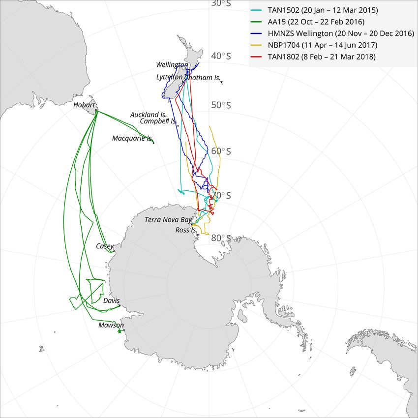
ble 1 and Fig. 1):1 diurnal variation in noise levels (Kotthaus et al., 2016). Due
to signal attenuation and noise, ceilometers cannot measure
– 2015 TAN1502 voyage of the NIWA ship RV Tangaroa
clouds obscured by a lower cloud and therefore cannot be
from Wellington, New Zealand, to the Ross Sea;
used for 1 : 1 comparison with model clouds without using a
– 2015–2016 voyages (V1–V3) of the Australian Antarc- lidar simulator, which accounts for this effect (Chepfer et al.,
tic Division (AAD) icebreaker Aurora Australis from 2008). The Lufft CHM 15k ceilometer operates in the near-
infrared spectrum at 1064 nm, measuring lidar backscatter up
1 The voyage name pattern is a 2–6 character ship name followed to a maximum height of 15 km, producing 1024 regularly
by a two-digit year and a two-digit sequence number. TANxxxx and spaced bins (about 15 m resolution). The sampling rate of
NBPxxxx are official voyage names, while HMNZSW16 and AA15 the instrument is 2 s. The Vaisala CL51 ceilometer operates
are names made for the purpose of this study. in the near-infrared spectrum at 910 nm. The sampling rate
https://doi.org/10.5194/acp-20-6607-2020 Atmos. Chem. Phys., 20, 6607–6630, 2020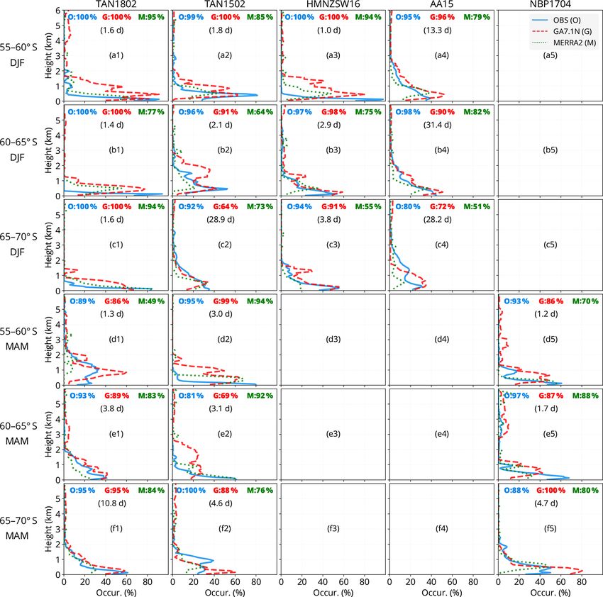
6610          P. Kuma et al.: Evaluation of Southern Ocean cloud in HadGEM3 and MERRA-2 using ship observations

Table 1. Table of voyages. The table lists voyages analysed in this study. Listed is the voyage name (Voyage), which is the official name
of the voyage or an abbreviation for the purpose of this study, ship name (Ship), organisation (Org.), start and end dates (yyyy-mm-dd) of
the voyage (Start, End), number of days spent at sea (Days), target region of the SO (Region), and maximum and minimum geographical
coordinates of the voyage track (Lat., Long.).

 Voyage               Ship                      Org.     Start        End           Days    Region             Lat.       Long.
 TAN1502              RV Tangaroa               NIWA     2015-01-20   2015-03-12      51    Ross Sea           41–75◦ S   162◦ E–174◦ W
 TAN1802              RV Tangaroa               NIWA     2018-02-08   2018-03-21      41    Ross Sea           41–74◦ S   170◦ E–175◦ W
 HMNZSW16             HMNZS Wellington          RNZN     2016-11-20   2016-12-20      20    Ross Sea           36–68◦ S   166–180◦ E
 NBP1704              RV Nathaniel B. Palmer    NSF      2017-04-11   2017-06-13      63    Ross Sea           53–78◦ S   163◦ E–174◦ W
 AA15 (AA V1–V3)      Aurora Australis          AAD      2015-10-22   2016-02-22     123    Indian O. sector   42–69◦ S   62–160◦ E

Figure 1. Map showing tracks of voyages used in this study. The ship observational dataset is comprised of five voyages between 2015 and
2018, spanning the months of November to June and latitudes between 40 and 78◦ S, of which data between 50 and 70◦ S are used in this
study.

of the instrument is 2 s and range is 7.7 km, producing 770            rection are derived) were retrieved to altitudes of about 10–
regularly spaced bins (10 m resolution).                               20 km, terminated by a loss of radio communication or bal-
   Radiosonde observations were performed on the TAN1802               loon burst.
and NBP1704 voyages south of 60◦ S. Temperature, pres-                    On the TAN1802 voyage we used iMet-1 ABx radioson-
sure, relative humidity and Global Navigation Satellite Sys-           des, measuring pressure, air temperature, relative humidity
tem (GNSS) coordinates (from which wind speed and di-                  and GNSS coordinates of the sonde (from which wind speed

Atmos. Chem. Phys., 20, 6607–6630, 2020                                                    https://doi.org/10.5194/acp-20-6607-2020
P. Kuma et al.: Evaluation of Southern Ocean cloud in HadGEM3 and MERRA-2 using ship observations                                     6611

Table 2. Table of deployments. The table cells indicate if data from a given instrument (row) was available from a voyage (column).

                          Instrument/voyage      AA15      TAN1502      HMNZSW16         NBP1704      TAN1802
                          Lufft CHM 15k                                       X              X            X
                          Vaisala CL51             X           X
                          iMet radiosondes                                                                X
                          Radiosondes (other)                                                X

and direction are derived). The sondes were launched three                – 1-hourly average Radiation Diagnostics (product
times a day at about 08:00, 12:00 and 20:00 UTC on 100 g                    “M2T1NXRAD.5.12.4”),
Kaymont weather balloons. They reached a typical altitude
of 10–20 km and then terminated by balloon burst or loss of               – 3-hourly instantaneous Assimilated Meteorological
radio communication. We used 10 s resolution profiles gen-                  Fields (product “M2I3NVASM.5.12.4”),
erated by the vendor-supplied iMetOS-II control software for
further processing.                                                       – 1-hourly instantaneous Single-Level Diagnostics (prod-
   Automatic weather station (AWS) data were available on                   uct “M2I1NXASM.5.12.4”),
the TAN1502, TAN1802 and NBP1704 voyages. These in-
cluded variables such as air temperature, pressure, sea sur-              – 3-hourly average Assimilated Meteorological Fields
face temperature, wind speed and wind direction. Voyage                     (product “M2T3NVASM.5.12.4”),
track coordinates were obtained from the ships’ GNSS re-
ceivers.                                                                  – 1-hourly average Single-Level Diagnostics (product
                                                                            “M2T1NXSLV.5.12.4”).
2.2   HadGEM3
                                                                           We used the “Radiation Diagnostics” in TOA outgoing
HadGEM3 (Walters et al., 2019) is a general circulation                 SW radiation evaluation (Sect. 5.1), the instantaneous “As-
model developed by the UK Met Office and the Unified                    similate Meteorological Fields” and “Single-Level Diagnos-
Model Partnership. It can be used in a “nudging” (Telford               tics” products to generate simulated ceilometer profiles and
et al., 2008) mode, in which winds and potential temperature            pseudo-radiosonde profiles (Sect. 5.2 and 5.3), and the av-
are relaxed towards the ERA-Interim reanalysis (Dee et al.,             erage “Assimilate Meteorological Fields” and “Single-Level
2011). The Met Office Global Atmosphere 7.1 (GA7.1) is the              Diagnostics” to generate zonal plane plots of thermodynamic
atmospheric component of HadGEM3 (Walters et al., 2019),                and cloud fields (Sect. 5.4). The four-dimensional MERRA-
based on the Unified Model (UM) version 11.0.                           2 fields were provided on pressure and model levels. For our
   The model runs used the HadISST sea surface tempera-                 analysis we chose to use the model-level products (72 levels)
ture dataset (Rayner et al., 2003) as lateral boundary con-             due to their higher vertical resolution compared to pressure-
ditions. The nudged simulations represent atmospheric dy-               level products. The analysed time period of MERRA-2 data
namics as determined by observations. The model was run                 was 2015–2018.
on a 1.875◦ × 1.25◦ (longitude × latitude) “N96” resolution
grid, which corresponds to a horizontal resolution of about             2.4   CERES
100 km × 140 km at 60◦ S and 85 vertical levels. The model
output fields were sampled every 6 h (instantaneous) and                The Clouds and the Earth’s Radiant Energy System (CERES)
daily (mean). In our analysis we used a nudged run of GA7.1             is a set of low Earth orbit (LEO) satellite instruments and
(“GA7.1N”) between the years 2015 and 2018, correspond-                 a dataset of SW and longwave (LW) radiation observations
ing to the ship observations.                                           (Loeb et al., 2018; Doelling et al., 2016). The CERES instru-
                                                                        ments (called FM1 to FM6) provide a continuous record of
2.3   MERRA-2                                                           observations since the first deployment on the Tropical Rain-
                                                                        fall Measuring Mission (TRMM) satellite in 1997 (Simpson
Modern-Era Retrospective analysis for Research and Appli-               et al., 1996) and have been flown on Terra, Aqua (Parkin-
cations (MERRA-2) is a reanalysis provided by the NASA                  son, 2003), the Suomi NPOESS Preparatory Project (Suomi
Global Modelling and Assimilation Office (Gelaro et al.,                NPP) and Joint Polar Satellite System-1 (JPSS-1) (Goldberg
2017). The reanalysis was chosen for its contrasting results            et al., 2013) satellites since. Currently CERES is considered
of TOA outgoing SW radiation bias in the SO compared to                 the best available global Earth radiation datasets and is often
GA7.1. As shown later (Fig. 3), its bias is positive rather than        used as the primary dataset for GCM tuning and validation
negative, when CERES is used as a reference.                            (Schmidt et al., 2017; Hourdin et al., 2017). We used the fol-
   We used the following products (Bosilovich et al., 2015):            lowing CERES products in our analysis:

https://doi.org/10.5194/acp-20-6607-2020                                                  Atmos. Chem. Phys., 20, 6607–6630, 2020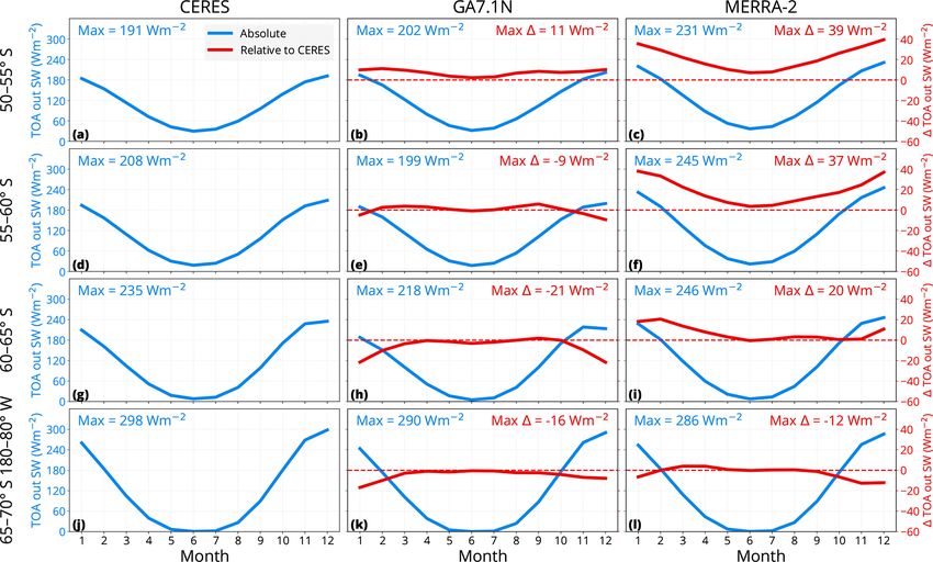
6612            P. Kuma et al.: Evaluation of Southern Ocean cloud in HadGEM3 and MERRA-2 using ship observations

    – CERES SYN1deg-Day edition 4A (configuration code           through the atmosphere, i.e. attenuation by hydrometeors and
      406406 and 407406) product of daily average radiation      air molecules and backscattering. COSP comprises multi-
      (“CERES SYN”),                                             ple instrument simulators, such as MODIS, ISCCP, MISR,
                                                                 CALIPSO and CloudSat. It has been used extensively by
    – CERES          EBAF-TOA           edition  4.1
                                                                 previous studies of model cloud, for example by Kay et al.
      (CERES_EBAF_Ed4.1) product of monthly energy-
                                                                 (2012), Franklin et al. (2013), Klein et al. (2013), Williams
      balanced average radiation (“CERES EBAF”).
                                                                 and Bodas-Salcedo (2017), Jin et al. (2017), and Schud-
   Due to the sun-synchronous orbits of the LEO satellite        deboom et al. (2018). COSP is planned to be used in the
platforms, the Flight Model (FM) instruments of CERES do         upcoming Coupled Model Intercomparison Project Phase 6
not capture the full diurnal variation in radiation. The EBAF    (CMIP6) (Webb et al., 2017).
and SYN1deg products are adjusted for diurnal variation by          For our analysis, we have developed a ground-based lidar
using 1-hourly geostationary satellite observations between      simulator by modifying the COSP ACTSIM spaceborne li-
60◦ S and 60◦ N, and use an algorithm to account for chang-      dar simulator (Chiriaco et al., 2006) (see the code and data
ing solar zenith angle and diurnal land heating. The CERES       availability section at the end of the document). This re-
EBAF-TOA edition 4.1 product is a Level 3B product, which        quired reversing of the vertical layers, as the surface lidar
means it has been globally balanced by ocean heat measure-       looks from the surface up rather than down from space to
ments using the Argo network (Roemmich and Team, 2009).          the surface, and changing the radiation wavelength affect-
                                                                 ing Mie scattering by cloud droplets and Rayleigh scattering
2.5    NSIDC sea ice concentration                               by air molecules. In this paper we present only a brief de-
                                                                 scription of the surface lidar simulator, with a more complete
We used the Near-Real-Time Defense Meteorological Satel-         description planned in an upcoming paper. The new simu-
lite Program (DMPS) Special Sensor Microwave Im-                 lator is made available as part of the Automatic Lidar and
ager/Sounder (SSMIS) Daily Polar Gridded Sea Ice Con-            Ceilometer Framework (ALCF) at https://alcf-lidar.github.io
centrations, version 1 product (NSIDC-0081) (Maslanik and        (last access: 1 June 2020).
Stroeve, 1999) provided by the National Snow and Ice Data           The recently introduced COSP version 2 (Swales et al.,
Center (NSIDC) to classify observations into those affected      2018) added support for a surface lidar simulator, although
and unaffected by sea ice. The sea ice concentration product     we believe our implementation, developed before COSPv2
has a resolution of 25 km × 25 km. We used a cutoff value        was available, is more complete in the present context due
of 15 % of sea ice concentration for the binary classification   to its treatment of Mie scattering at wavelengths other than
of sea ice, in line with previous studies (Comiso and Nishio,    532 nm (the wavelength of the CALIPSO lidar). Previously,
2008).                                                           a surface lidar simulator based on COSP has been used by
                                                                 Chiriaco et al. (2018) and Bastin et al. (2018). A ground-
3     Methods                                                    based radar simulator in COSP has also recently been imple-
                                                                 mented (Zhang et al., 2018).
3.1    Lidar simulator                                              The surface lidar simulator takes model cloud liquid and
                                                                 ice mixing ratios, cloud fraction and thermodynamic pro-
The CFMIP Observation Simulator Package (COSP) (Bodas-           files as the input, and calculates vertical profiles of attenuated
Salcedo et al., 2011), a set of instrument simulators devel-     backscatter. This can be done either by running the simula-
oped by the Cloud Feedback Model Intercomparison Project         tor “online” within the model code or “offline” on the model
(CFMIP), was extended with a surface lidar simulator and         output. We used the offline approach in our analysis.
used to produce virtual lidar measurements from model fields
(Kuma et al., 2020a). Resampling, noise reduction and cloud      3.2   Lidar data processing
detection were performed on observational and (where appli-
cable) model lidar data in a consistent way to reduce struc-     Lidar data in this study came from two different instruments:
tural uncertainty (see Sect. 3.2). The schematic in Fig. 2       Lufft CHM 15k and Vaisala CL51 ceilometers and the li-
shows the processing pipeline utilised in this study.            dar simulator. These instruments use different output for-
   COSP was originally developed as a satellite simula-          mats, wavelengths, sampling rates and range bins, as pre-
tor package whose aim is to produce virtual satellite (and       viously noted. Backscatter and derived fields such as CBH
more recently ground-based) observations from atmospheric        are provided in the firmware-generated data products, but
model fields in order to improve comparisons of model out-       the backscatter is uncalibrated and the derived fields such
put with observations (Bodas-Salcedo et al., 2011). This         as cloud detection are based on instrument-dependent al-
approach is required because physical quantities derived         gorithms. Therefore, we performed consistent subsampling,
from satellite observations generally do not directly corre-     noise reduction and cloud detection on data from both instru-
spond to model fields. COSP accounts for the limited view        ments, and applied the same methods to the lidar simulator
of the satellite instrument by calculating radiative transfer    output. As part of the processing we developed a publicly

Atmos. Chem. Phys., 20, 6607–6630, 2020                                            https://doi.org/10.5194/acp-20-6607-2020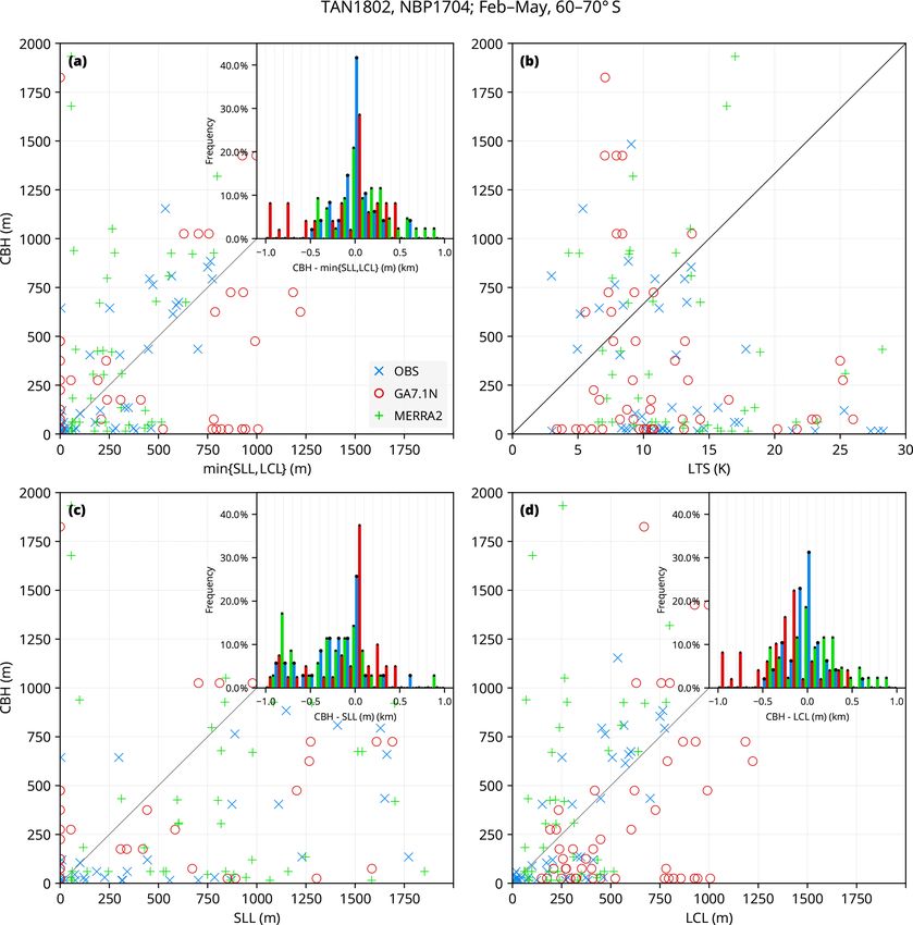
P. Kuma et al.: Evaluation of Southern Ocean cloud in HadGEM3 and MERRA-2 using ship observations                                     6613

Figure 2. Schematic of the processing pipeline utilised in this study to produce lidar and radiosonde statistics from observations and model
data.

available tool called cl2nc (“CL to NetCDF”) for converting             rate was 2 s) and subtracting the range-scaled noise mean
the Vaisala CL51 ceilometer data format to NetCDF (see the              from the backscatter. We then used the range-scaled noise
code and data availability section at the end of the document).         standard deviation (σ ) for cloud detection: a bin was consid-
                                                                        ered cloudy if the calibrated backscatter minus 3σ exceeded
3.2.1   Calibration                                                     20 × 10−6 m−1 sr−1 . This threshold was chosen subjectively
                                                                        so that cloud was visually well separated from other features,
The backscatter profiles produced by the Lufft CHM 15k                  such as boundary layer aerosol and noise on backscatter pro-
and Vaisala CL51 ceilometers are not calibrated to physical             file plots. The same threshold was used on both the observa-
units, even though they are expressed in metres per steradian           tions and output from the COSP surface lidar simulator and
(m−1 sr−1 ). To calibrate these backscatter fields we used the          thus should cause little bias.
method described by O’Connor et al. (2004). This method
uses the lidar ratio (LR) to calculate a calibration factor based       3.2.3    Model lidar data processing
on a known value of the LR in fully scattering cloudy scenes
(18.8±0.8 sr), such as thick stratocumulus clouds, which are            We used the same sampling rate (5 min) and model lev-
common over the SO. We applied this technique by using                  els as range bins on the surface lidar simulator output. For
visually identified scenes and choosing a calibration factor            each vertical profile we used model data at the same loca-
which achieves the known value. Due to the nature of the                tion as the ship and the same time relative to the start of
conditions (LR can be highly variable even in thick cloud               the year. Model data were selected using nearest-neighbour
scenes), the calibration is likely accurate to only about 50 %          interpolation. The model resolution is lower than the dis-
of the backscatter value. We do not expect this to have a se-           tance travelled by the ship in 5 min, therefore the same model
rious impact on the accuracy of cloud detection completed               data were used multiple times to generate consecutive pro-
in this study, largely because the predominantly low cloud              files. However, we also used the SCOPS (Webb et al., 2001)
tends to cause backscatter orders of magnitude greater than             subcolumn generator included in COSP to generate 10 ran-
clear air and because of the very large differences in cloud            dom samples of cloud for each profile based on cloud frac-
occurrence between the observations and models.                         tion and the maximum–random cloud overlap assumption
                                                                        (Bodas-Salcedo, 2010). The lidar simulator processes each
3.2.2   Subsampling, noise removal and cloud detection                  sample individually. The resulting cloud occurrence is calcu-
                                                                        lated as the average of the 10 samples. The lidar simulator
In order to simplify further processing and increase the                does not generate noise, and therefore we did not perform
signal-to-noise ratio, we subsampled the ceilometer obser-              any noise removal on the simulated profiles, but we used the
vations at a sampling rate of 5 min by averaging multiple               same threshold of 20 × 10−6 m−1 sr−1 and vertical bins of
profiles, and vertically averaging on regularly spaced 50 m             50 m for detecting cloud (as used on the observations). For
bins. We expect that in most cases cloud was almost con-                the MERRA-2 cloud occurrence analysis, we applied the li-
stant on this timescale and vertical scale, and therefore we            dar simulator on the 3-hourly instantaneous Assimilated Me-
were not averaging together different cloud types or clear              teorological Fields (M2I3NVASM.5.12.4) product.
and cloudy profiles. At the same time as subsampling, we
performed noise removal by estimating the noise distribution
(mean and standard deviation) based on returns in the upper-
most range bins (i.e. 300 samples over 5 min when sampling

https://doi.org/10.5194/acp-20-6607-2020                                                   Atmos. Chem. Phys., 20, 6607–6630, 2020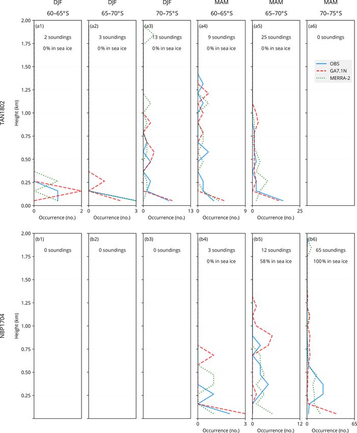
6614            P. Kuma et al.: Evaluation of Southern Ocean cloud in HadGEM3 and MERRA-2 using ship observations

4     Spatio-temporal subsets investigated                        coming solar radiation in DJF. The bias displays very simi-
                                                                  lar geographical pattern on the annual scale, DJF and MAM.
Because our observational dataset does not span the entire        The bias is much lower in MAM compared to DJF due to
geographical area of the SO and all months of the year, and       lower incoming solar radiation.
the atmospheric conditions in the SO are geographically vari-         We chose 1 January 2018 as a representative day in DJF
able, we subset the datasets into a number of geographical        to show the daily scale. On the daily scale (Fig. 3j, k, l), the
regions (by latitude) and time periods (by season). The geo-      patterns are closely linked to synoptic features. The region on
graphical regions investigated are 50–75◦ S by 5◦ of latitude,    the eastern side of the Antarctic Peninsula shows the greatest
and the temporal periods investigated are austral summer of       negative bias in the models. The relatively zonally symmetric
December, January, February (DJF) and autumn months of            annual and seasonal means suggest that there is not a signif-
March, April, May (MAM).                                          icant need for subsetting by longitude and that latitude aver-
   We do not use data from 70 to 75 and 50 to 55◦ S in all        ages can be very useful in identifying the key features of the
parts of the analysis. The data from 70 to 75◦ S are likely       SW radiation biases. The daily synoptic features are gener-
affected by circulation induced by land near the Ross Sea         ally well correlated between CERES and the models, which
(Coggins et al., 2014) and therefore may not be representa-       is expected in nudged model runs and reanalyses. MERRA-2
tive of the SO in general. This decision builds on the analysis   has greater TOA outgoing SW radiation than GA7.1N on all
detailed in Jolly et al. (2018) which shows a significant gra-    three time periods presented here. Considering that cloud is
dient in cloud properties between the Ross Ice Shelf and the      the dominant factor affecting SW radiation in the SO, this
Ross Sea and strong influences associated with synoptic con-      can only be associated with either cloud cover that is too
ditions. The data from 50 to 55◦ S were relatively sparse (the    high or cloud albedo that is too high. GA7.1N reflects too
ships spent relatively little time passing through these lati-    little SW radiation south of 60◦ S and too much radiation
tudes). Radiosonde observations were only available south         north of 60◦ S (Fig. 3b, e, h). MERRA-2 reflects too much
of 60◦ S.                                                         SW radiation in most of the SO, except for coastal regions
   There is likely temporal variability present within the DJF    of Antarctica (approx. 65–70◦ S) and the eastern side of the
and MAM time periods, but we decided to limit the num-            Antarctic Peninsula. The opposite sign of SW radiation bias
ber of temporal subsets to maintain a reasonable quantity         in GA7.1N compared to MERRA-2 suggests that contrasting
of observations in each subset. The magnitude of the SO           the two models could be useful for uncovering the cause of
TOA outgoing SW radiation bias is primarily modulated by          the bias.
incoming solar radiation, which is the highest in DJF. The            Figure 4 shows line plots of zonal mean reflected SW
voyages do not uniformly cover all geographical regions or        radiation and bias relative to CERES by month in multi-
time periods, with the largest number of observations in the      ple latitude bands between 50 and 70◦ S, with the southern-
Ross Sea sector south of New Zealand (TAN1802, TAN1502,           most band 65–70◦ S limited to 180–80◦ W to avoid covering
HMNZSW16 and NBP1704), followed by the Indian Ocean               land areas in Antarctica. The annual cycle follows the ex-
sector south of Western Australia (AA15). Temporally, the         pected seasonal pattern modulated by varying incoming so-
voyage observations mostly cover summer to autumn months          lar radiation with maxima of reflected radiation in December
of the year.                                                      and maxima of bias in December and January. The Antarc-
                                                                  tic sea ice extent, at its minimum in February and peaking
                                                                  in September, is also likely a secondary modulating factor
5     Results                                                     of the TOA outgoing SW radiation at higher latitudes. The
                                                                  models represent the seasonal pattern well but differ substan-
5.1    Shortwave radiation balance                                tially during the periods of peak incoming solar radiation.
                                                                  The GA7.1N model (Fig. 4b, e, h, k) exhibits bias ranging
Figure 3 shows TOA outgoing SW radiation in CERES,                from −21 to +11 W m−2 . The bias is positive north of 55◦ S
GA7.1 and MERRA-2. We present this panel plot in order            and negative south of this latitude, with the greatest absolute
to evaluate how well GA7.1N and MERRA-2 are performing            bias between 60 and 65◦ S. MERRA-2 displays a clearly dif-
in terms of SW radiation bias in the SO relative to CERES.        ferent bias from GA7.1N, ranging from −12 to 39 W m−2
This analysis assumes that CERES is a good observational          (Fig. 4c, f, i, l). The peak SW bias in MERRA-2 is positive
reference, although it is affected by errors of lower order of    for latitudes north of 65◦ S and negative south of this lat-
magnitude (2.5 W m−2 “regional monthly uncertainty”; Loeb         itude. The absolute bias in MERRA-2 is much larger than
et al., 2018, Sect. 4a.). The plots reveal a relatively zonally   in GA7.1N north of 60◦ S and similar to GA7.1N south of
symmetric pattern of negative and positive bias on the an-        this latitude. Therefore, the MERRA-2 results are valuable
nual (Fig. 3b, c) and seasonal (Fig. 3e, f, h, i) timescales.     for contrasting with GA7.1. The strong latitudinal variation
GA7.1N shows predominantly negative bias, while MERRA-            in the TOA outgoing SW radiation bias is important to take
2 shows predominantly positive bias. The annual average is        into consideration. Previous studies of SO clouds often did
dominated by the bias in DJF due to the relatively strong in-     not discern different latitudes.

Atmos. Chem. Phys., 20, 6607–6630, 2020                                             https://doi.org/10.5194/acp-20-6607-2020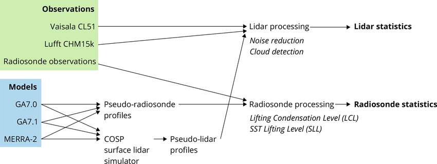
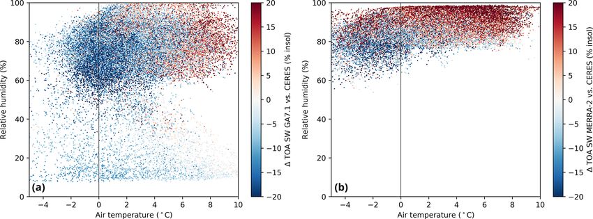
P. Kuma et al.: Evaluation of Southern Ocean cloud in HadGEM3 and MERRA-2 using ship observations                              6615

Figure 3. Geographical distribution of the TOA outgoing SW radiation in CERES, GA7.1N and MERRA-2. The plots show global all-sky
SW radiation as annual (2015–2018; a–c), seasonal (2015–2018 DJF, MAM; d–i) and daily (1 January 2018; j–l) mean. The blue–red colour
map shows bias relative to CERES (b, c, e, f, h, i), while the grayscale colour map shows absolute values (a, d, g, j, k, l).

Figure 4. Zonal means of the TOA outgoing SW radiation in CERES, GA7.1N and MERRA-2 during the years 2015–2018 in 5◦ latitude
bands between 50 and 70◦ S. The plots show monthly zonal mean TOA outgoing SW radiation (blue) and its difference relative to CERES
(red) as a function of month. Also shown are the maxima (“max”) and the difference from CERES (“max 1”).

   Figure 5 shows a scatter plot of the TOA outgoing SW ra-          of negative bias at temperature around 0 ◦ C in GA7.1N and
diation bias in GA7.1N and MERRA-2 as a function of near-            −2 ◦ C in MERRA-2 and a cluster of positive bias at higher
surface air temperature and relative humidity between 55 and         temperatures. This is consistent with the latitudinal depen-
70◦ S in January 2018. The bias is predominantly negative in         dence of bias in both models shown above.
GA7.1N and positive MERRA-2. There is a strong cluster

https://doi.org/10.5194/acp-20-6607-2020                                              Atmos. Chem. Phys., 20, 6607–6630, 2020
6616 P. Kuma et al.: Evaluation of Southern Ocean cloud in HadGEM3 and MERRA-2 using ship observations
Figure 5. Scatter plot of SW radiation bias in (a) GA7.1N and (b) MERRA-2 grid cells between 55 and 70◦ S in January 2018. Each point
represents a daily average of SW radiation bias as a function of near-surface air temperature and near-surface relative humidity. The bias is
expressed as a percentage of the incoming solar radiation in the grid cell. The points are a random sample of 100 000 points.
5.2 Cloud occurrence in model and observations marginally more consistent between the models and observa-
tions in terms of the cloud occurrence profile, but the cloud
To understand how clouds contribute to the SW bias, we ex- cover is still markedly underestimated.
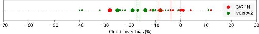
amine cloud cover and cloud occurrence as a function of Figure 7 shows the model subsets of Fig. 6 as points by
height in the models and observations. Figure 6 shows cloud their cloud cover bias relative to observations. It can be seen
occurrence profiles derived from ceilometer observations on that GA7.1N underestimates cloud cover by about 4 % and
different voyages and GA7.1N and MERRA-2 model output MERRA-2 by 16 % when non-weighted averages are con-
derived via the COSP surface lidar simulator, in subsets by sidered, and by 9 % (GA7.1N) and 18 % (MERRA-2) when
latitude and season. Most notably, the observed cloud cover weighted averages are considered.
is consistently very high in the observations (80 %–100 %) Due to the nature of the lidar measurements, middle to
for all periods and latitude bands examined and greater than high clouds may be obscured by low clouds, as the laser
90 % in most of the subsets. This finding differs substan- signal is quickly attenuated by thick cloud. Therefore, the
tially from the modelled cloud cover derived via the sur- lack of clouds above 2 km in the plots does not imply that no
face lidar simulator, which ranges between 69 % and 100 % clouds are present. The lidar simulator, however, ensures un-
in GA7.1N, and is about 4 %–9 % lower than observations biased 1 : 1 comparison with observations by accounting for
across the subsets. The cloud cover in MERRA-2 is also the signal attenuation.
lower than observed and much lower than in GA7.1N, span- The results demonstrate the value of surface cloud mea-
ning 51 %–95 %. Only in four subsets is the cloud cover surements in the SO relative to satellite measurements such
greater in GA7.1N than observed, and only in one subset is as CloudSat and CALIPSO, which would likely provide a bi-
the cloud cover greater in MERRA-2 than observed (out of ased sample of these clouds because of “ground clutter” and
21 subsets). Our analysis therefore shows that cloud cover is obscuration by higher-level clouds, respectively (Alexander
underestimated in both GA7.1N and MERRA-2 in the eval- and Protat, 2018).
uated geographical regions and seasons.
Examination of the vertical distributions in Fig. 6 shows 5.3 Radiosonde observations
that observations have a strong predominance of cloud be-
low 2 km and peaking below 500 m in most subsets, includ- We use radiosonde measurements performed on TAN1802
ing a substantial amount of surface-level fog in some sub- and NBP1704 to evaluate boundary layer properties and cor-
sets. In contrast, GA7.1N and MERRA-2 simulate clouds at relate them with clouds observed by a ceilometer. We com-
a higher altitude, peaking at about 500 m and generally the pare the observations with “pseudo-radiosonde” profiles ex-
peak is higher than in observed clouds. Especially, clouds tracted from model fields at the same location and time. The
below 500 m and fog appear to be lacking in the models. location is based on the GNSS coordinates of the ship at the
The subsets in Fig. 6 are derived from uneven length of time of the balloon launch (the balloon trajectory length was
ship observations (1.0–28.9 d) due to the limited availability generally not long enough to span multiple model grid cells
of data. The longer subsets (Fig. 6a4, b4, c2, c4, f1) appear in the lower troposphere).
Atmos. Chem. Phys., 20, 6607–6630, 2020 https://doi.org/10.5194/acp-20-6607-2020P. Kuma et al.: Evaluation of Southern Ocean cloud in HadGEM3 and MERRA-2 using ship observations 6617 Figure 6. Cloud occurrence frequency as a function of height derived from ceilometer observations (OBS) and model fields (GA7.1N and MERRA-2). The observational and model data were subsetted by latitude and season (DJF, MAM) along the voyage track. The numbers at the top of each panel show total (vertically integrated) cloud cover and the number of days the ship spent passing through the spatio-temporal subset. The height in the plots is limited to 6 km. There was no significant amount of cloud detected above this level. Figure 7. Cloud cover bias in models relative to observations. The points represent subsets as in Fig. 6. The size of the circles is proportional to the number of days of observations in the subset. The solid lines are averages, and dashed lines are averages weighted by the number of days the ship spent passing through the spatio-temporal subset. https://doi.org/10.5194/acp-20-6607-2020 Atmos. Chem. Phys., 20, 6607–6630, 2020
6618          P. Kuma et al.: Evaluation of Southern Ocean cloud in HadGEM3 and MERRA-2 using ship observations

   We define a new quantity “SST lifting level” (SLL) de-            tity, with peak at about 300 m. GA7.1N and MERRA-2 rep-
rived from SST and boundary layer atmospheric potential              resent the distribution over sea ice relatively poorly.
temperature, defined as the level to which an air parcel with
the same temperature as SST, rising from the sea surface,            5.4    Zonal plane comparison of GA7.1N and MERRA-2
would rise adiabatically by buoyancy. That is, it is the level
closest to the surface at which potential temperature is equal       In order to better understand the differences in the SW radia-
to SST, provided the air parcel is permitted to rise to this level   tion bias between GA7.1N and MERRA-2, we inspect zonal
by buoyancy (otherwise the air parcel does not rise and SLL          plane plots of cloud occurrence and thermodynamic fields
is 0 m). This quantity is applicable in sea-ice-free conditions      of the models in DJF 2017/18 and 1 January 2018 (Fig. 10).
in the SO, when cold Antarctic air is warmed by the open sea         The figure shows seasonal and daily average cloud liquid and
surface and is lifted by buoyancy until it reaches a limit im-       ice mixing ratio contours plotted over two different back-
posed by the atmospheric stability of the atmosphere. Along-         grounds: potential temperature and relative humidity (RH).
side the lifting condensation level (LCL), we found SLL to           The daily average plots (Fig. 10c, d) show a very pronounced
be a useful quantity for evaluation of CBH. The authors are          difference between the cloud liquid amount between the two
not aware of any previous use of SLL, but this definition is         models, with MERRA-2 simulating a much greater amount
supported by observations (see below).                               of cloud liquid. In contrast, GA7.1N simulates cloud with
   Apart from SLL and LCL, we also use the lower tropo-              ice, which are nearly absent in MERRA-2 at the chosen con-
spheric stability (LTS) (Klein and Hartmann, 1993). LTS is           tour levels. The liquid content is generally concentrated near
defined as the difference between potential temperature at           SLL in MERRA-2 but much less so in GA7.1N, where SLL
700 hPa and sea level pressure (Klein and Hartmann, 1993).           is often at 0 m. The cloud ice in GA7.1N generally has sig-
It has been used in multiple previous studies (Williams et al.,      nificantly greater vertical extent than the cloud liquid. These
2006; Franklin et al., 2013; Williams et al., 2013; Naud et al.,     differences are also present on the seasonal scale (Fig. 10a,
2014).                                                               b). The difference in potential temperature between the mod-
   Figure 8 shows the observed and modelled relation-                els is relatively small. GA7.1N, however, shows a slightly
ship between CBH and the minimum of SLL and LCL                      higher potential temperature. The RH field is very different
(“min{SLL,LCL}”), LTS, SLL and LCL. A large fraction of              between GA7.1N and MERRA-2, with MERRA-2 simulat-
the observed points (OBS) in Fig. 8a lie close to the origin         ing higher RH by about 10 %.
(40 % in the first 100 m in observations vs. 26 % and 17 % in           Perhaps most interestingly, the vertically integrated liquid
GA7.1N and MERRA-2, respectively), which suggests that               and ice content (Fig. 10i, j) is very different between the
near zero min{SLL,LCL} is a good indicator of fog or very            models. Both models simulate almost the same liquid + ice
low cloud, a relationship not well represented in the mod-           total, but the phase composition of cloud in GA7.1N is ma-
els. The remaining observed points show a close equivalence          jority ice, while in MERRA-2 it is almost entirely liquid.
between min{SLL,LCL} and CBH, while the models do not
represent this equivalence well. The histogram in Fig. 8a re-
veals that about 42 % of observed profiles have CBH within           6     Discussion
100 m of min{SLL,LCL}, while only about 28 % of GA7.1N
and 21 % of MERRA-2 profiles do.                                     The TOA outgoing SW radiation assessment shows that the
   Using SLL or LCL as a predictor for CBH individu-                 models exhibit monthly average biases of up to 39 W m−2
ally resulted in a weaker relationship than min{SLL,LCL}:            (MERRA-2, 50–55◦ S in December), and that these biases
25 % and 31 % of OBS profiles have CBH within 100 m of               have a significant latitudinal dependency, with the opposite
SLL and LCL, respectively (Fig. 8c, d). This suggests that           sign of bias between different latitude bands. In GA7.1N
min{SLL,LCL} is more strongly related to CBH than SLL                the bias is predominantly negative, while in MERRA-2 the
or LCL individually. Figure 8b shows CBH as a function               bias is predominantly positive. A similar pattern of bias is
of LTS. LTS does not display a good predictive ability for           present in both models. The bias is positive north of 55◦ S
CBH in this dataset, with the exception of very stable pro-          (65◦ S) in GA7.1N (MERRA-2) and negative south of this
files (LTS > 15 K), when observed CBH was below 250 m in             latitude. This finding is consistent with Schuddeboom et al.
all but one case.                                                    (2019), who observed opposite sign of SW cloud radiative
   Figure 9 shows the distribution of min{SLL,LCL} derived           effect south and north of 55◦ S in GA7.1.
from radiosonde observations and model fields. In observa-              A very similar geographical pattern of bias is present in
tions, the quantity almost consistently peaks near the ground        DJF and MAM, suggesting that similar cloud biases are
and reaches up to 1.5 km in ice-free cases (Fig. 9a1–a5, b4).        present in both seasons. This is also supported by Fig. 6,
GA7.1N represents this distribution relatively well. This is         which does not display a significant difference in observed
not the case with MERRA-2, which is less likely to peak near         cloud occurrence and bias in the models between DJF and
the ground (Fig. 9a3, a5, c4). The sea-ice cases (Fig. 9b5, b6)      MAM. Consistent with the maximum of incoming solar ra-
show markedly different observed distribution of the quan-           diation, December and January were found to be the months

Atmos. Chem. Phys., 20, 6607–6630, 2020                                                 https://doi.org/10.5194/acp-20-6607-2020
P. Kuma et al.: Evaluation of Southern Ocean cloud in HadGEM3 and MERRA-2 using ship observations 6619
Figure 8. Scatter plots of radiosonde measurements on the TAN1802 and NBP1704 voyages between February and May and 60 and 70◦ S
latitude. Corresponding profiles from GA7.1N and MERRA-2 are selected, i.e. having the same geographical coordinates and the same time
of the year. Each point on the scatter plots represents a radiosonde profile. The plots compare three datasets: observations (OBS), GA7.1N
and MERRA-2. The radiosonde observations are matched with ceilometer (OBS) and COSP-based CBH (GA7.1N and MERRA-2). Panel (a)
shows the points as a function of min{SLL, LCL} and CBH. The inset histogram shows distribution of the difference of CBH and min{SLL,
LCL} in bins of 100 m, where each bin contains three bars for the three datasets. Panels (b), (c) and (d) show the points as a function of LTS,
SLL and LCL, respectively.
with the greatest absolute bias in the models. Therefore, fix- in MERRA-2, and positive bias is predominantly correlated
ing the representation of clouds in the SO in these months is with higher temperature.
relatively more important than in other months.
Figure 5 suggests that the bias correlates not only with lat-
itude but also with near-surface air temperature. The negative
bias is strongly clustered around 0 ◦ C in GA7.1N and −2 ◦ C
https://doi.org/10.5194/acp-20-6607-2020 Atmos. Chem. Phys., 20, 6607–6630, 20206620 P. Kuma et al.: Evaluation of Southern Ocean cloud in HadGEM3 and MERRA-2 using ship observations
Figure 9. Histogram of min{SLL,LCL} derived from radiosonde observations (OBS) on TAN1802 and NBP1704, and the equivalent profiles
in GA7.1N and MERRA-2. Shown are subsets by latitude between 60 and 75◦ S and seasons DJF and MAM. The numbers at the top of each
panel indicate the number of profiles that make up the histogram and the percentage of sea ice cases determined from NSIDC satellite-derived
sea ice concentration.
Atmos. Chem. Phys., 20, 6607–6630, 2020 https://doi.org/10.5194/acp-20-6607-2020P. Kuma et al.: Evaluation of Southern Ocean cloud in HadGEM3 and MERRA-2 using ship observations 6621 Figure 10. Zonal plane plot of cloud liquid and ice mixing ratios in GA7.1N and MERRA-2 at 60◦ S. The cloud liquid and ice mixing ratios are plotted as contours on top of the potential temperature fields (a–d) and relative humidity fields (e–h). SLL is indicated by a white line. Panels (a), (b), (e) and (f) show a seasonal average in DJF 2017/2018, and panels (c), (d), (g) and (h) show a daily average on 1 January 2018. Panels (i) and (j) show the column-integrated values of cloud liquid and ice water as a function of longitude corresponding to the plots above. All liquid shown in the plots is supercooled (air temperature is less than 0 ◦ C everywhere). The ship-based lidar cloud occurrence revealed close to tence of synoptic situations). The subsets show a relatively 100 % cloud cover in multiple subsets. Subsetting allowed consistent cloud occurrence profile peaking below 500 m and us to identify whether the cloud cover is substantially dif- almost zero above 2 km (possibly also due to obscuration of ferent by latitude and season and also sample independent lidar signal by lower clouds). The models generally do not weather situations (it is expected that cloud occurrence pro- reproduce this profile well. Apart from underestimating the files are highly correlated over several days due to persis- total cloud cover, the peak of cloud occurrence in the models https://doi.org/10.5194/acp-20-6607-2020 Atmos. Chem. Phys., 20, 6607–6630, 2020
6622          P. Kuma et al.: Evaluation of Southern Ocean cloud in HadGEM3 and MERRA-2 using ship observations

is higher than observed. Improving the cloud profile repre-       in GA7.1, which contrasts with the negative bias south of the
sentation in the models is likely key for improving the SW        latitude, is important because it places a limit on the appli-
radiation bias.                                                   cability of other studies, which used SO observational data
   The effect of clouds on SW radiation is the product of         from regions north of 55◦ S (Lang et al., 2018).
cloud cover (the fraction of the sky containing clouds) and          In Sect. 5.3 we show that min{SLL,LCL} has a stronger
cloud albedo (the fraction of SW radiation reflected by the       equivalence to CBH than SLL, LCL individually or LTS.
clouds). With our ship-based lidar observations we measured       This relationship becomes quite notable when examining the
cloud cover (total, and cloud cover as a function of height),     individual voyage radiosonde profiles (not presented here).
while we did not measure cloud albedo. The cloud cover            We hypothesise that the theoretical reason for this relation-
was almost consistently underestimated in both GA7.1N and         ship is the following. When SLL is higher than LCL, an air
MERRA-2 across all latitudes. At the same time, the satel-        parcel warmed by the sea surface to temperature close to
lite observations show that MERRA-2 reflects too much all-        SST rises by buoyancy past LCL to a level with the equiv-
sky SW radiation. Therefore, the cloud albedo in MERRA-2          alent potential temperature. The water vapour starts to con-
must be too high in order to cause too much all-sky SW ra-        densate at LCL (assuming enough cloud condensation nuclei
diation reflection despite the lack of cloud cover. This effect   are present at 100 % saturation), forming cloud with CBH
is visible on the daily scale in Fig. 3j–l, where the individ-    equal to LCL. If SLL is lower than LCL, the air parcel rises
ual clouds in MERRA-2 appear significantly brighter than          to the level of equivalent potential temperature, where air
on satellite observations.                                        lifted from the sea surface eventually accumulates, poten-
   Remarkably, the observed cloud occurrence profiles ap-         tially forming cloud if enough moisture is transported from
pear to be similar between the DJF and MAM seasons and            the sea surface. The models do not represent the observed re-
latitude bands between 55 and 70◦ S (Fig. 6): if we focus on      lationship well and improving this relationship may be one
the subsets with more than 10 d (Fig. 6a4, b4, c2, c4, f1),       way of improving the cloud simulation.
i.e. not heavily skewed toward a single weather situation, we        Considering the strong observed relationship between
find that they are all characterised by a peak below 500 m        min{SLL,LCL} and CBH (CBH tends to occur at the
of 25 %–60 % and falling to near-zero above 2–3 km, some-         same level as min{SLL,LCL}), we evaluated the dis-
times with a minor secondary peak between 1 and 2 km. The         tribution of min{SLL,LCL} in the models in compari-
simulated profiles show a slightly higher altitude of the pri-    son with radiosonde observations (Fig. 9). We found that
mary peak between 0 and 1 km, underestimated in MERRA-            GA7.1N represents this distribution relatively well in sea-
2 by up about two-thirds and falling to near-zero between 2       ice-free cases, while MERRA-2 underestimates cases when
and 3 km without any substantial secondary peak. The total        min{SLL,LCL} was near the surface. This may be the rea-
cloud fraction appears to be more strongly underestimated         son for the underestimation of very low cloud and fog in
at high latitudes in GA7.1N in DJF, by 8 %–28 % (Fig. 6c2,        this model identified in the comparison with lidar observa-
c4) vs. 8 % (Fig. 6b4). This is an important consideration in     tions. Therefore, improving the distribution of the quantity
connection with the SW radiation bias, which shows a strong       in MERRA-2 may lead to improvement of low cloud simu-
latitudinal gradient of the TOA outgoing SW radiation bias        lation.
in the models (Figs. 3, 4). Based on the presented results,          It is interesting to contrast our results with previous studies
a plausible explanation for the SW radiation bias could be        which used cyclone compositing for the TOA SW radiation
overestimation of cloud albedo north of about 55◦ S (65◦ S)       bias evaluation in GCMs. We cannot make substantial con-
in GA7.1N (MERRA-2) causing positive TOA outgoing SW              clusions from our results on how much of the model bias is
radiation bias north of this latitude and underestimation of      attributable to cyclones. It appears, however, that the cloud
cloud cover over the whole SO causing negative TOA outgo-         cover and cloud liquid and ice mixing ratio bias in GA7.1N
ing SW radiation bias south of this latitude.                     is systematic rather than isolated to cyclonic activities due to
   In the ship observations we found a notable correspon-         its relative consistency across spatio-temporal subsets in the
dence between CBH, SLL and LCL. Boundary layer ther-              high-latitude SO. This does not rule out even greater biases
modynamics, which determine the lifting levels, are a plausi-     related to cyclonic sectors. Specifically, Bodas-Salcedo et al.
ble driver of cloud formation in the absence of other forcing.    (2014) evaluated a large set of models, including HadGEM2-
We examined SLL in models and radiosonde observations             A, a predecessor model to HadGEM3, likely affected by sim-
and found differences which are likely too small to explain       ilar biases and found that about 80 % of grid cells south of
the cloud occurrence differences between the models and           55◦ S could be classified as affected by a cyclone, and that
ceilometer observations. Bodas-Salcedo et al. (2012), in their    these grid cells were responsible for the majority of the to-
analysis of an earlier version of the GA model (GA3.0) using      tal SW radiation bias. Moreover, their cyclone compositing
cyclone composites also noted that biases in thermodynam-         showed that the bias in HadGEM2-A was largely negative
ics are not likely to explain the SW radiation bias but may       in the cold quadrants, and near zero in the warm quadrants.
still play a significant role. The presence of positive TOA       Their results also indicate a strong contrast in SW bias south
outgoing SW radiation bias in the SO between 50 and 55◦ S         and north of 55◦ S, similar to the result we found in GA7.1N.

Atmos. Chem. Phys., 20, 6607–6630, 2020                                             https://doi.org/10.5194/acp-20-6607-2020
You can also read