Vehicle-induced turbulence and atmospheric pollution
←
→
Page content transcription
If your browser does not render page correctly, please read the page content below
Atmos. Chem. Phys., 21, 12291–12316, 2021
https://doi.org/10.5194/acp-21-12291-2021
© Author(s) 2021. This work is distributed under
the Creative Commons Attribution 4.0 License.

Vehicle-induced turbulence and atmospheric pollution
Paul A. Makar, Craig Stroud, Ayodeji Akingunola, Junhua Zhang, Shuzhan Ren, Philip Cheung, and Qiong Zheng
Air Quality Modelling and Integration Section, Air Quality Research Division, Atmospheric Science and Technology
Directorate, Environment and Climate Change Canada, 4905 Dufferin Street, Toronto, Ontario, M3H 5T4, Canada

Correspondence: Paul A. Makar (paul.makar@canada.ca)

Received: 6 December 2020 – Discussion started: 5 January 2021
Revised: 7 May 2021 – Accepted: 9 June 2021 – Published: 17 August 2021

Abstract. Theoretical models of the Earth’s atmosphere ad-       1   Introduction
here to an underlying concept of flow driven by radiative
transfer and the nature of the surface over which the flow
is taking place: heat from the sun and/or anthropogenic          A common and ongoing problem with theoretical descrip-
sources are the sole sources of energy driving atmospheric       tions of the Earth’s atmosphere is a dichotomy in the rep-
constituent transport. However, another source of energy is      resentation of turbulent transport, between the turbulence
prevalent in the human environment at the very local scale       estimated in weather forecast models, and the turbulence
– the transfer of kinetic energy from moving vehicles to         required for accurate simulations in air-quality forecast
the atmosphere. We show that this source of energy, due          models. Representations of atmospheric turbulence used in
to being co-located with combustion emissions, can influ-        weather forecast and climate models have focused on pa-
ence their vertical distribution to the extent of having a       rameterizations of “sub-grid-scale turbulence”: descriptions
significant influence on lower-troposphere pollutant concen-     of the storage and release of energy derived from incom-
trations throughout North America. The effect of vehicle-        ing solar radiation and anthropogenic heat release, physical
induced turbulence on freshly emitted chemicals remains no-      factors in the built environment, and the transfer of sensi-
table even when taking into account more complex urban           ble and latent heat between the built environment and the
radiative transfer-driven turbulence theories at high resolu-    atmosphere. These efforts adhere to an underlying concept
tion. We have designed a parameterization to account for         of radiatively driven flow: heat transfer from the sun and/or
the at-source vertical transport of freshly emitted pollutants   anthropogenic sources being the source of energy behind at-
from mobile emissions resulting from vehicle-induced tur-        mospheric motions. There has been considerable research fo-
bulence, in analogy to sub-grid-scale parameterizations for      cused on improving the understanding of radiatively driven
plume rise emissions from large stacks. This parameteriza-       flow in urban areas (e.g., the advection and diffusion associ-
tion allows vehicle-induced turbulence to be represented at      ated with buildings and street canyons, Mensink et al., 2014;
the scales inherent in 3D chemical transport models, allow-      urban heat island radiative transfer theory, Mason, 2000; ef-
ing this process to be represented over larger regions than      forts to increase 3D model vertical and horizontal resolution
is currently feasible with large eddy simulation models. In-     in order to better capture the physical environment, Leroyer
cluding this sub-grid-scale parameterization for the vertical    et al., 2014). However, when these physical models of tur-
transport of emitted pollutants due to vehicle-induced turbu-    bulence are applied to problems involving the emissions,
lence in a 3D chemical transport model of the atmosphere         transport, and chemistry of atmospheric pollutants, predicted
reduces pre-existing North American nitrogen dioxide biases      surface concentrations of emitted pollutants may be biased
by a factor of 8 and improves most model performance scores      high and concentrations aloft biased low, indicating the pres-
for nitrogen dioxide, particulate matter, and ozone (for exam-   ence of missing additional sources of atmospheric dispersion
ple, reductions in root mean square errors of 20 %, 9 %, and     (Makar et al., 2014; Kim et al., 2015). Despite ongoing work
0.5 %, respectively).                                            to improve the turbulence schemes in meteorological mod-
                                                                 els (Makar et al., 2014; Hu et al., 2013; Klein et al., 2014),
                                                                 computational predictive models of atmospheric pollution

Published by Copernicus Publications on behalf of the European Geosciences Union.
12292                                             P. A. Makar et al.: Vehicle-induced turbulence and atmospheric pollution

typically make use of a constant “floor” or “cut-off” in the      et al., 2018). However, the application of this information
thermal turbulent transfer coefficients provided by weather       has been limited up to now to theoretical and computational
forecast models, sometimes with higher values of this cut-        models of the near-roadway environment and large eddy sim-
off over urban compared to rural areas (Makar et al., 2014),      ulation models with horizontal domains of a few kilometers
in an attempt to compensate for apparent insufficient verti-      in extent.
cal mixing of chemical tracers. The turbulent mixing in these        Regional air-quality models also have vertical resolution
physical descriptions, while capable of reproducing observed      in the tens of meters near the surface, suggesting the poten-
meteorological conditions, does not explain lower concentra-      tial for vehicle-induced turbulence (VIT) to influence turbu-
tion observations of emitted atmospheric pollutants.              lent mixing out of the lowest model layer(s). Here we demon-
   Large stack sources of pollutants provide a useful analogy     strate that this sub-grid-scale vertical transport process, due
in investigating a potential cause of this discrepancy. Emis-     to its highly localized spatial nature (over roadways), has a
sions from these sources occur at high temperatures, lofting      disproportionate impact on the vertical distribution and trans-
their emitted mass high into the atmosphere as a result of        port of freshly emitted chemical tracers. A comparable sub-
buoyancy effects. However, the physical size of the stacks        grid-scale process which has a similar influence on pollu-
(< 10 m diameter) is much smaller than the grid cell size         tants are the emissions from large stacks noted above (Gor-
used in regional models (kilometers to tens of kilometers). In    don et al., 2018; Akingunola et al., 2018). Accurate estima-
order to capture the rapid vertical redistribution of emissions   tion of pollutant concentrations from the latter sources must
from large stacks, sub-grid-scale parameterizations are used,     take into account the at-source buoyancy and exit velocity of
in which buoyancy calculations are performed to determine         high-temperature exhaust to determine the vertical distribu-
plume heights, which are then used to determine the distribu-     tion of fresh emissions. Similarly, our work focuses on deter-
tion of freshly emitted pollutants (Briggs, 1982, 1984; Gor-      mining the local lofting of pollutants from and due to moving
don et al., 2018; Akingunola et al., 2018). For large stack       vehicles, in order to adequately represent the at-source verti-
emissions, these parameterizations account for the effect of      cal distribution of their emissions, on the larger scale.
the addition of energy (the hot exhaust gas) on the local dis-       The extent of the vertical influence of VIT varies depend-
tribution of pollutants and are essential in estimating initial   ing on the configuration of vehicles on the roadway. From ob-
vertical distribution of those pollutants.                        servations taken from a trailer following an isolated passen-
   In this work, we investigate the potential for another type    ger van (Rao et al., 2002) and large eddy simulation (LES)
of at-source energy to influence the vertical distribution of     and other computational fluid dynamics (CFD) models of in-
freshly emitted pollutant concentrations: the addition of ki-     dividual vehicles (Kim, 2011; Y. Kim et al., 2016), the ver-
netic energy due to the displacement of air during the passage    tical distance over which VIT can be distinguished from the
of vehicles on roadways. Roadway observations in the 1970s        background for isolated, individual vehicles (i.e., the mixing
showed that this transferred energy has a significant influ-      length) is on the order of 2.5 to 5.13 m. However, as we show
ence on the transport of primary pollutants released from ve-     in the Methodology and the Results sections, for observa-
hicle exhaust, with vehicle passage being associated with “a      tions of ensembles of vehicles in traffic (Gordon et al., 2012;
distinct bulge in the high frequency range of the wind spec-      Miller et al., 2018) and large eddy and other computational
trum”, “corresponding to eddy sizes on the order of a few         fluid dynamics simulations of ensembles of vehicles (Y. Kim
metres” (Rao et al., 1979). The same work found that the          et al., 2016; Woodward et al., 2019; Zhang et al., 2017), the
variation in the concentration of non-reactive tracers could      mixing lengths associated with VIT are larger and on the or-
be attributed to wakes behind moving vehicles. Subsequent         der of tens of meters, to as much as 41 m. The vertical ex-
theoretical development led to the creation of the roadway-       tent of the impacts of alternating low and high areas of sur-
scale models describing turbulence within a few tens of me-       face roughness have been shown to create downwind internal
ters around and above roadways, in turn used to estimate          boundary layers to even more significant heights in the atmo-
the very local-level impact of vehicles on emitted pollu-         sphere (e.g., 300 m, Bou-Zeid et al., 2004, their Fig. 12), sug-
tant concentrations (Eskridge and Catalano, 1987). These          gesting that impacts on the lower boundary layer due to the
models showed that near-roadway concentrations of emit-           alternating roughness elements (in our case, vehicles versus
ted pollutants were highly dependent on vehicle speed, with       roadways) is not unreasonable. We also show in the Method-
over a factor of 2 reduction in emission-normalized pollu-        ology section that the impact of VIT within the context of
tant concentrations being associated with an increase in ve-      an air-quality model is via changes to the vertical gradient of
hicle speed from 20 to 100 km h−1 (Eskridge et al., 1991).        the thermal turbulent transfer coefficients; the gradient of the
With the advent of portable, very high time resolution 3D         sum of the natural turbulence and VIT terms allows VIT to
sonic anemometers, the turbulent kinetic energy of individ-       influence vertical mixing, even when model vertical resolu-
ual vehicles could be measured directly, either aboard an in-     tion is relatively coarse.
strumented trailer towed behind a vehicle (Rao et al., 2002)         LES and other CFD models have shown the importance
or through instrumentation mounted aboard a laboratory fol-       of VIT towards modifying local values of turbulent kinetic
lowing other vehicles in traffic (Gordon et al., 2012; Miller     energy, as noted in the references above. However, these

Atmos. Chem. Phys., 21, 12291–12316, 2021                                         https://doi.org/10.5194/acp-21-12291-2021
P. A. Makar et al.: Vehicle-induced turbulence and atmospheric pollution                                                 12293

models require relatively small grid cell sizes compared to       2     Methodology
regional chemistry models (centimeters to tens of meters)
and time steps to allow forward time-stepping predictions         2.1    Theoretical development
of future meteorology and chemistry. These constraints in
turn severely limit the size of the domain in which they          In contrast to the very local-resolution “roadway” models
can be applied, and the processing time for simulations for       used to examine the impact of vehicle motion on pollutant
these reduced domains can be very high. For example, the          concentration (Eskridge and Catalano, 1987; Eskridge et al.,
FLUENT model was used by Y. Kim et al. (2016) with an             1991) and computational fluid dynamics modeling of vehicle
adaptive mesh with a minimum cell size of 1 cm, with a            turbulence (Kim, 2011; Y. Kim et al., 2016; Woodward et al.,
100 m×20 m×20 m domain, while Woodward et al.’s (2019)            2019; Zhang et al., 2017), 3D models of atmospheric pollu-
implementation of FLUENT had a cell size of 50 cm, oper-          tion (Galmarini et al., 2015) have horizontal grid cell sizes
ating in a domain of 600 000 nodes (a volume of 75 000 m3 ),      of 1 km to tens of kilometers, and thus emissions and vertical
and an adaptive time step limited by a Courant number of 5.       transport associated with roadways must be approached from
The latter criterion implies a computation time step of less      the standpoint of sub-grid-scale parameterizations. Measure-
than 0.09 s for a 100 km h−1 vehicle (or wind) speed, while       ments of the turbulent kinetic energy (TKE) associated with
a 1 cm grid cell size implies a computation time step of less     vehicles are usually available on a “per-vehicle” or “per ve-
than 1.8 × 10⁻³ s time step. Similarly, the LES model em-         hicle within an ensemble” basis. These observations provide
ployed by Zhang et al. (2017) utilized a 1 m × 2 m × 1 m cell     the average on-road TKE per vehicle passing a point per unit
size and a computation time step of 0.03 s. Other LES models      time (Gordon et al., 2012; Miller et al., 2018) and/or the
have larger horizontal resolution but are limited in horizontal   shape of the enhanced TKE cross section in the plane per-
domain extent relative to regional chemical transport mod-        pendicular to the vehicle’s motion (Rao et al., 2002). A sub-
els (example LES models incorporating gas-phase chemistry         grid-scale parameterization linking these scales is therefore
include Vinuesa and Vilà-Guerau de Arellano (2005), with          necessary in order to study the impacts of VIT on the verti-
a 50 m horizontal resolution and a 3.2 km × 3.2 km domain;        cal redistribution of freshly emitted pollutants and hence on
Ouwersloot et al. (2011), with a 50 m horizontal resolution       large-scale atmospheric chemistry and transport. Sub-grid-
and a 12.8 km × 12.8 km domain; Li et al. (2016), with a          scale parameterizations are commonly used in atmospheric
150 m horizontal resolution and a 14.4 km×14.4 km horizon-        models of weather forecasting to provide the rates of change
tal domain; and S. W. Kim et al. (2016), with a 66.6 m hori-      in processes which occur at scales smaller than the model’s
zontal resolution and a 6.4 km × 6.4 km domain). In contrast,     horizontal and/or vertical resolution, cloud formation, and
a 3D regional chemical transport model typically operates         buoyant plume rise from large stacks being a common exam-
over a domain with may be continental in extent (the sim-         ple for model grid cell sizes of 10 km or more (Kain, 2004;
ulations described here have a 10 km × 10 km and 2.5 km ×         Briggs, 1982, 1984; Gordon et al., 2018; Akingunola et al.,
2.5 km horizontal resolutions with 7680 km × 6380 km and          2018).
1300 km×1050 km domains, respectively). The limiting hor-            Three separate problems must be addressed in the con-
izontal resolution for regional chemical transport models is      struction of such a VIT parameterization for atmospheric
on the order of kilometers, with a limiting vertical resolution   chemical transport models, specifically the following:
on the order of tens of meters and time steps on the order            1. What is the relationship governing the decrease in VIT
of 1 min. These limits for regional chemical transport mod-              with increasing distance (height) from the vehicles?
els are a function of the need to provide chemical forecasts
                                                                      2. How can observation data, in units of vehicles per unit
over a relatively large region, within a reasonable amount of
                                                                         time, be related to variables more commonly available
current supercomputer processing time (the chemical calcu-
                                                                         for regional chemical transport models?
lations typically taking up the bulk of the processing time).
LES models are capable of capturing VIT effects (Y. Kim et            3. How can VIT be incorporated into a regional model
al., 2016; Zhang et al., 2017; Woodward et al., 2019), and               in a manner that only the emissions due to vehicles
their results have been used here in developing our param-               are affected, given that the vehicle-induced turbulence
eterization but are constrained by current computer capac-               will have the most significant impact on emissions from
ity from being applied for the larger-scale domains required             moving vehicles due to the relatively low area fraction
in regional- to continental-scale air pollution simulations. A           of roadway area within a given grid cell?
“scale gap” exists between LES and regional chemical trans-       We address each of these issues in the sub-sections that fol-
port models – for regional chemical transport models, param-      low.
eterizations of the physical processes such as VIT, resolvable
at the high resolution of LES models, are therefore required.     2.2    Changes in VIT with height
In return, these parameterizations allow the relative impact
of the parameterized processes on the larger domain sizes of      Measurements of TKE behind a passenger van (Rao et al.,
regional chemical transport models to be determined.              2002) typically show a smooth distribution, with TKE de-

https://doi.org/10.5194/acp-21-12291-2021                                        Atmos. Chem. Phys., 21, 12291–12316, 2021
12294                                                        P. A. Makar et al.: Vehicle-induced turbulence and atmospheric pollution

creasing both above and below the height of the upper trail-
ing edge of the moving vehicle. Similar results have been
seen from very high-resolution computational fluid dynam-
ics modeling of the flow around individual vehicles, although
the shape of the vehicle and the arrangement of vehicles on
the roadway can have a strong influence on the location of
the maximum and shape of the vertical profile in TKE (Kim,
2011; Y. Kim et al., 2016). We examined four data sets (the
observations of Rao et al., 2002, and the LES modeling of
Y. Kim et al., 2016; Woodward et al., 2019; Zhang et al.,
2017) to evaluate the extent to which a Gaussian distribution
may be used to represent the decrease in VIT with height
above moving vehicles, as well as examining the expected
range of mixing lengths which may result from VIT. A Gaus-
sian distribution of TKE with height is given by Eq. (1),
where Iq (z) is the time-integrated added TKE value for ve-
hicle type q with height z (m2 s−1 ), hq is the height of the
vehicle, and Aq and σq are numerical constants:
                                  (z−hq )2                                   Figure 1. Example of length scales associated with an ensemble of

             Aq               −
                                    2σq2                                     vehicles (after Y. Kim et al., 2016; Fig. 14). TKE contours along
Iq (z) = q            e                          .                     (1)
             2π σq2                                                          dashed lines were extracted and fit to Eqs. (1) and (2) for Table 1.
                                                                             Note that the length scale of turbulence immediately behind the
Equation (1) may be rewritten as                                             leading vehicle, a large transport truck, is only 5.13 m, while the
                                      2                                     length scale immediately behind the trailing vehicle in the ensem-
   √
                      Aq       z − hq                                        ble (an identical transport truck) is 14.73 m.
ln    2π Iq (z) = ln       −             .                             (2)
                      σq         2σq2

Equation     (2) shows that values of −(z − hq )2 versus                     the figure). Increases in downwind turbulent length scales as-
    √                                                                        sociated with vehicles moving in close ensembles are a com-
ln( 2π Iq (z)), with the values of z taken from vertical pro-
files of Iq (z) in the literature, will yield a slope of 2σ1 2 and           mon feature in the literature.
                                                                   q            This analysis (see Table 1) shows that a Gaussian distribu-
                          A
an intercept of ln( σqq ), and the correlation coefficient for this          tion accounts for much of the variability in TKE with height
relationship may be used to judge the accuracy of the use                    (correlation coefficients of 0.54 to 0.99), and under realis-
of a Gaussian distribution to describe the decrease in TKE                   tic traffic conditions, the mixing lengths increase in size and
with height above moving vehicles. The resulting relation-                   may be considerably larger than those of isolated vehicles.
ships may also be used to describe the vertical mixing length,                  Two VIT mobile laboratory studies (Gordon et al., 2012;
defined “as the diameter of the masses of fluid moving as a                  Miller et al., 2018) observed vehicle-per-second TKE for ve-
whole in each individual case; or again, as the distance tra-                hicles moving in ensembles along multilane roadways, ag-
versed by a mass of this type before it becomes blended in                   gregated by vehicle classes using the same methodology, to
with neighbouring masses” (Prandtl, 1925; Bradshaw, 1974).                   derive formulae for the net TKE added by VIT at 4 and 2 m
Here we assume that this blending has occurred at the height                 (the height of the instrumentation used in these studies). We
at which the Gaussian has dropped to 0.01 of the value at                    combine these data here to determine the change in VIT with
z = hq (i.e., the value of z at which VIT has reached 1 % of                 height. Setting E as the TKE added due to the vehicles, two
its maximum value (i.e., e−(z−hq ) /(2σq ) = 0.01).
                                                     2   2                   formulae result as follows:
   An example of the analysis used to construct Table 1 ap-                  E(4 m) = 1.8Fc + 2.2Fm + 20.4Ft ,
pears in Fig. 1 for a CFD example for an ensemble of vehi-                   E(2 m) = 2.4Fc + 6.2Fm + 14.8Ft ,                               (3)
cles, taken from the literature (Y. Kim et al., 2016). In this fig-
ure, contours of TKE are shown as solid lines. TKE values as                 where E(4 m) and E(2 m) are the TKE added driving within
a function of height at three locations behind the trucks were               the ensemble at 4 and 2 m elevation from these two studies
used to determine σq and hence estimate the length scale via                 (m2 s−2 ) and Fc , Fm , and Ft are the number of passenger cars
Eqs. (1) and (2). A notable feature of this example is the sub-              and mid-sized (vans, flatbed pickup trucks, and SUVs) and
stantial increase in length scale which occurs between the                   large vehicles (10 to 18 wheel heavy-duty vehicles) traveling
initial vehicle (a transport truck) and subsequent downwind                  past a given point on the highway per second. The numer-
vehicles (compare the height of TKE contours, and the result-                ical coefficients are the time-integrated TKE values (Iq ) at
ing length scales in Fig. 1, between the left and right sides of             the two heights (m2 s−1 ). An alternative approach would be

Atmos. Chem. Phys., 21, 12291–12316, 2021                                                     https://doi.org/10.5194/acp-21-12291-2021
P. A. Makar et al.: Vehicle-induced turbulence and atmospheric pollution                                                                                                     12295

Table 1. Gaussian distribution fits of VIT TKE drop-off with height, from observation and CFD studies.

  Study, case                                                                                       Slope       Intercept            R2                          Mixing length
                                                                                                                                                          (z−hq )2

                                                                                                                                                        −     2
                                                                                                                                                            2σq
                                                                                                                                             (z at e                  = 0.01), m
  Isolated vehicles
  Rao et al. (2002), cube van, 80.5 km h−1 , hq = 2 m                                             2.2452          1.8534        0.9856                                        3.53
  Rao et al. (2002), cube van, 48.3 km h−1 , hq = 2 m                                             1.0230          1.4969        0.9709                                        4.22
  Y. Kim et al. (2016), lead automobile, hq = 1.5 m                                               4.6431          3.9013        0.8845                                        2.50
  Y. Kim et al. (2016), lead diesel cargo truck, hq = 4 m                                         3.6143          4.2223        0.9355                                        5.13
  Vehicle ensembles
  Y. Kim et al. (2016), automobile immediately following                                       0.073529           4.1144        0.9801                                        9.41
  lead diesel cargo truck, hq = 1.5 m
  Y. Kim et al. (2016), second automobile, following                                             0.47337          3.9275         1.00a                                        4.60
  lead diesel cargo truck, hq = 1.5 m
  Y. Kim et al. (2016) second diesel cargo truck, hq = 4 m                                       0.04070          4.7935        0.5424                                       14.64

  Woodward et al. (2019) vehicle ensembleb , hq = 1.5 m,                                         0.01916        −1.2402         0.9135                                       17.01
  parallel to flow, right lane
  Woodward et al. (2019) vehicle ensembleb , hq = 1.5 m,                                         0.01155        −1.4532         0.7543                                       21.46
  parallel to flow, left lane
  Woodward et al. (2019) vehicle ensembleb , hq = 1.5 m,                                       0.012489         −1.4766         0.9667                                       20.70
  transverse to flow, right lane
  Woodward et al. (2019) vehicle ensembleb , hq = 1.5 m,                                     0.0098094          −1.7815         0.9536                                       23.16
  transverse to flow, left lane
  Zhang et al. (2017), VS1: hq = 1.6 m, vehicle speed = 9 km h−1 ,                           0.0029165            5.1706        0.6614                                       41.24
  wind 11 km h−1
  Zhang et al. (2017), VS2: hq = 1.6 m, speed = 36 km h−1 ,                                    0.005158           5.0964        0.8306                                       31.38
  wind 11 km h−1
  Zhang et al. (2017), VS3: hq = 1.6 m, vehicle speed = 36 km h−1 ,                            0.007298           6.3394        0.9006                                       26.62
  wind 36 km h−1
  Zhang et al. (2017), VS4: hq = 1.6 m, vehicle speed = 36 km h−1 ,                            0.005411           5.6387        0.9339                                       30.67
  wind 36 km h−1
  Zhang et al. (2017), VS5: hq = 1.6 m, vehicle speed = 36 km h−1 ,                            0.003478           4.3150        0.8574                                       37.89
  wind 54 km h−1
a Note that only two contour lines were available for retrieving TKE and height values from this vehicle within Fig. 14 of Y. Kim et al. (2016); while the correlation coefficient is
formally unity, this is a two-point line.
b Woodward et al. (2019) Fig. 21 turbulent velocity components in the parallel and transverse directions were squared, and distances were scaled to give equivalent distances from
wind-tunnel to ambient environment.

to make use of vehicle speed data within each grid cell and                                   the vehicles travel across one dimension of a grid cell allows
parameterizations utilizing vehicle speed (Di Sabatino et al.,                                us to generate the Fc values required to estimate TKE. Note
2003; Kastner-Klein et al., 2003) to construct TKE additions                                  that vehicle speed is implicit in this methodology utilizing
due to the sub-grid-scale roadways. However, vehicle speed                                    vehicle kilometer traveled (VKT) – higher speeds will result
information is not currently readily available on a gridded                                   in a greater number of vehicle kilometers traveled per unit
hourly basis, while estimates of vehicle kilometer traveled                                   time and hence higher TKE values. As in the above discus-
are available in gridded form due to their use in emissions                                   sion, we assume a Gaussian distribution of the coefficients of
processing, and making the simple scaling assumption that                                     the TKE equations of Eq. (3) with height for each vehicle,

https://doi.org/10.5194/acp-21-12291-2021                                                                          Atmos. Chem. Phys., 21, 12291–12316, 2021
12296                                                        P. A. Makar et al.: Vehicle-induced turbulence and atmospheric pollution

where hq = 1.5, 1.9, and 4.11 m for cars, mid-sized vehicles,                      two variable in two unknowns (Aq , σq ) problem we find val-
and trucks, respectively, with each of the 2 and 4 m values of                     ues of lc , lm , and lt of 13.56, 6.25, and 11.28 m, respectively.
the coefficients of Eq. (3) being used to determine the corre-                     These values are based on observed traffic conditions and fall
sponding values of Aq and σq of Eq. (1), (i.e., q = c, m, t).                      well within the range of mixing lengths provided for vehi-
The resulting height-dependent formulae may be used to re-                         cle ensembles in Table 1; however, we note that they are a
place the coefficients of Eq. (3), leading to the following for-                   source of uncertainty, with the percent uncertainties (Gor-
mula for the net turbulent kinetic energy associated with the                      don et al., 2012) associated with the 4 m values at ±52 %,
number of vehicles in transit along a given stretch of roadway                     ±157 %, and ±12 % for cars, mid-sized vehicles, and trucks,
at a given time:                                                                   respectively. The relatively low values of lm and high uncer-
                                                                                   tainties in the corresponding mid-sized vehicle per-vehicle
                       −2.40×10⁻² (z−1.5)2

Enet (z) = 2.43Fc e                                                                estimates of TKE relative to the other vehicle types are likely

                              −1.18×10⁻¹ (z−1.9)2
                                                                                  the result of a combination of small sample size (Gordon
              + 15.58Fm e
                                                                                   et al., 2012, noted the relative proportion of the three ve-
                             −3.61×10⁻² (z−4.11)2

              + 20.43Ft e                             .                      (4)   hicle classes as 89.9 % cars, 4.8 % mid-sized vehicles, and
                                                                                   5.3 % trucks) and the variety of ensemble versus isolated ve-
Most 3D chemical transport models make use of some varia-                          hicles sampled (noting the variation in Table 1 for vehicles
tion in “K-theory” diffusion to link turbulent kinetic energy                      within the smaller vehicle size classes). Additional observa-
to mixing, with the vertical mixing of a transported variable                      tions of vehicle turbulence are clearly needed, particularly
c due to turbulence at heights z being related to the thermal                      in the region above the largest vehicles on the road (4.1 m),
turbulent transfer coefficient K via                                               using remote-sensing techniques such as Doppler lidar, in or-
∂c      ∂

              ∂c
                                                                                  der to improve mixing length estimates. However, the values
    =       K       .                                     (5)                      used here are reasonable with respect to the available data,
 ∂t    ∂z     ∂z
                                                                                   and while they likely overestimate the mixing length asso-
Finite differences and tridiagonal matrix solvers are usually                      ciated with isolated vehicles (Rao et al., 2002; Y. Kim et al.,
used to forward integrate Eq. (5). For example, the solver                         2016), they likely underestimate the mixing length of ensem-
used in the Global Environmental Multiscale – Modelling                            bles of vehicles (Y. Kim et al., 2016), particularly for ensem-
Air-quality and CHemistry (GEM-MACH) model uses the                                bles moving within street canyons (Woodward et al., 2019;
following finite difference for the spatial derivatives (both                     Zhang et al., 2017). The latter represent the some of the spe-
spatial derivatives are O 1σ 2 , the derivatives are carried                       cific regions where vehicle emissions are likely to dominate.
out in, and the K values are transformed into, σ = PP0 coor-                          We derive the following formula for the addition to the
                                                                                   thermal turbulent transfer coefficient associated with vehicle
dinates as K̃, where P is the pressure and P0 is the surface
                                                                                   passage as a function of height:
pressure):
                                                                                                  lc Fc + lm Fm + lt Ft
                                                                                   KVIT (z) = 0.4
cin+1 − cin                                                                                           Fc + Fm + Ft
    1t

                                                                                                         −2      2


     1 K̃

                          ci+1 −ci

                                                            c −c
                                                                                   · 2.43Fc e −2.40×10 (z−1.5)
     2   i+1 + K̃i        σi+1 −σi       − 21 K̃i + K̃i−1 σii −σi−1
                                                                 i−1
 =                                                                       .
                                                                                                     −1.18×10⁻¹ (z−1.9)2

                              σi+ 1 − σi− 1                                          + 15.58Fm e
                                  2       2
                                                                             (6)                                              21
                                                                                                    −3.61×10⁻² (z−4.11)2

                                                                                     + 20.43Ft e                                    .            (8)
Note in Eq. (6) that the prognostic values of K calculated
by the weather forecast model are on the same vertical levels
                                                                                   The use of Eq. (8) must be undertaken with care. Like most
as concentration; values of the additional component of K
                                                                                   regional air-quality models, the vertical resolution of GEM-
associated with VIT must therefore be calculated for model
                                                                                   MACH used here is relatively coarse (the first four model
layers as opposed to layer interfaces.
                                                                                   layer midpoints are located approximately 24.9, 99.8, 205.0,
   K and E may be linked through the relationship of Prandtl,
                                                                                   and 327.0 m above the surface). Layer midpoint values must
where l is a characteristic length scale:
                                                                                   be representative of the layer resolution in order to describe
          √
K = 0.4l E.                                               (7)                      the impact of VIT on the layer. A simple linear interpolation
                                                                                   between the peak values of KVIT and the first model inter-
As was done for Table 1, we have chosen this value on a per-                       face will overestimate the impact of VIT within the lowest
vehicle basis as the vertical location at which the Gaussian                       model layer, while the use of Eq. (8) for the midpoint value
profiles derived above reach 0.01 (i.e., 1 %) of their maxi-                       alone will underestimate the influence of VIT within the low-
mum value. Using each of the coefficient values of Eq. (3)                         est part of the first model layer. The best representation of a
at the two heights, in conjunction with Eq. (1) treated as a                       sub-grid-scale scalar quantity within a discrete model layer is

Atmos. Chem. Phys., 21, 12291–12316, 2021                                                            https://doi.org/10.5194/acp-21-12291-2021
P. A. Makar et al.: Vehicle-induced turbulence and atmospheric pollution                                                     12297

its vertical average within that layer. Here, we calculate the      2.4   Relating VIT to available gridded data – vehicle
vertically integrated average of Eq. (8) within each model                kilometer traveled
layer, to provide the best estimate of the impact of VIT, to
within the vertical resolution of the model.                        Along individual roadways, Eq. (8) makes use of Fc , Fm ,
                                                                    and Ft observations at points along roadways within a grid
                                                                    cell, hence deriving local estimates of VIT. These data are
2.3   VIT and model vertical resolution
                                                                    currently difficult to obtain for large-scale applications, and
                                                                    hence we have turned to secondary sources of information
The issue of the vertical extent of the impact of VIT is worth      to estimate these three terms. VKT is used for estimating on-
considering in the context of model layer thickness. Given          road vehicle emissions at jurisdiction level (e.g., county level
that the vertical length scale of added VIT is on the order         for the US and province level for Canada) for national emis-
of tens of meters, as denoted in the studies quoted herein,         sions inventories. Emissions processing systems used for air-
it is reasonable to question whether the added turbulence           quality models make use of spatial surrogates to help de-
should be expected to have an impact on the dispersion of           termine the spatial allocation of the mass emitted from dif-
pollutants. This apparent contradiction is easily resolved by       ferent types of vehicles on different roadways (Adelman et
noting (1) that the turbulence due to VIT is added as an            al., 2017). The same set of surrogates is used for calculat-
addition to the pre-existing “meteorological” thermal turbu-        ing VKT (km s−1 ) for each grid cell of the model domain
lent transfer coefficient (with the net turbulence profile, not     (varying by hour of day and day of week, for each of the
the VIT alone, determining its impact on vertical mixing)           three vehicle categories listed (see Fig. 3), in turn provid-
and (2) that the impact of this net turbulence does not de-         ing diurnal variations in VIT matching traffic flow. The data
pend just on the magnitude of the net coefficients of thermal       shown are derived from 2006 Canadian (Brett Taylor, Na-
turbulent transfer, but also on their vertical gradient. This       tional Pollution Release Inventory, Environment and Climate
second point can be illustrated by expanding the diffusion          Change Canada, personal communication, 2019) and 2011-
equation using the chain run of calculus (i.e., (∂c)/(∂t) =         based projected 2017 US VKT (EPA, 2017). Note that for the
(∂)/(∂z)(Knet (∂c)/(∂z)) = Knet (∂ 2 c)/(∂z2 )+(∂Knet )/(∂z)·       10 km grid cell size used here, values of Fc , Fm , and Ft may
(∂c)/(∂z)) and the aid of an example, shown in Fig. 2. Fig-         be derived by dividing these numbers by 10. The largest con-
ure 2 displays examples of cases where the concentration            tribution to total vehicle kilometer traveled is by the “cars”
gradient and natural thermal turbulent transfer coefficient         class (Fig. 3a) due to their greater numbers (the originating
both decrease linearly with height (Fig. 2a and b) and where        study (Miller et al., 2018) found that 89.9 % of vehicles mea-
the concentration gradient decreases with height while the          sured were cars), followed by trucks (Fig. 3c; 5.3 % of ve-
natural thermal turbulent transfer coefficients increase with       hicles measured) and mid-sized vehicles (Fig. 3b; 4.8 % of
height (Fig. 2c and d). The added KVIT is shown as a blue           vehicles measured).
dashed line, and the net vertical thermal turbulent transfer is        These VKT data may be linked to the above VIT formula
shown as a red line. Figure 2a and c depict these curves at a       in Eq. (8), provided the distance each vehicle is traveling
high vertical resolution, while Fig. 2b and d depict them at        within that grid cell is known. Here, we have made two addi-
a low (regional model) resolution. Note that in the latter, the     tional assumptions. The first assumption is that each vehicle
vehicle-induced addition to the net thermal turbulent transfer      carries out a simple transit of the cell – the distance traveled
coefficient depicted in Fig. 2a and c lies entirely within the      is the cell size. While this may be a reasonable first-order
lowest model layer of Fig. 2b and d. In both Fig. 2a and b,         approximation, we note that it has limitations: for example,
the impact of KVIT is to slow the build-up of near-surface          when the number of vehicles on the roads overwhelm the ca-
concentrations. In both Fig. 2c and d, the impact of KVIT           pacity of the roads (rush-hour traffic jams), the distance trav-
is to more rapidly vent near-surface concentrations further         eled decreases. However, under these circumstances the VKT
up into the atmosphere. That is, at both high and low reso-         values will also decrease; the impact of rush-hour conditions
lution, KVIT affects near-surface concentrations, due to the        should to some extent be included within the VKT estimates
vertical gradient of (∂Knet /∂z). Centered difference calcula-      available for emissions processing systems. The second as-
tions for the low-resolution case are shown in Fig. 2b and d        sumption is that the VKT contributions within a grid cell are
to illustrate the point that gradients in low vertical-resolution   additive – i.e., that their numbers may be added via the “F ”
net diffusivity result in reductions in the lowest model layer      terms in Eq. (8) (Gordon et al., 2012; Miller et al., 2018), an
trapping and increases in venting from this lowest layer. In        assumption found to be accurate in CFD modeling (Y. Kim
both of these cases, the addition of vehicle turbulence to the      et al., 2016). Note that this assumption may result in over-
lowest model layer changes the gradient of the net thermal          estimates of the net TKE – a better methodology for future
turbulent transfer coefficient, in turn leading to reduced sur-     work would be to collect and make use of statistics of vehicle
face concentrations. The above example illustrates the man-         density by roadway type within each grid cell. However, we
ner in which VIT may have an impact even on relatively low          note that assuming that vehicles are evenly distributed over
vertical model resolution.                                          roadways in a grid cell would result in a net underestimate

https://doi.org/10.5194/acp-21-12291-2021                                         Atmos. Chem. Phys., 21, 12291–12316, 2021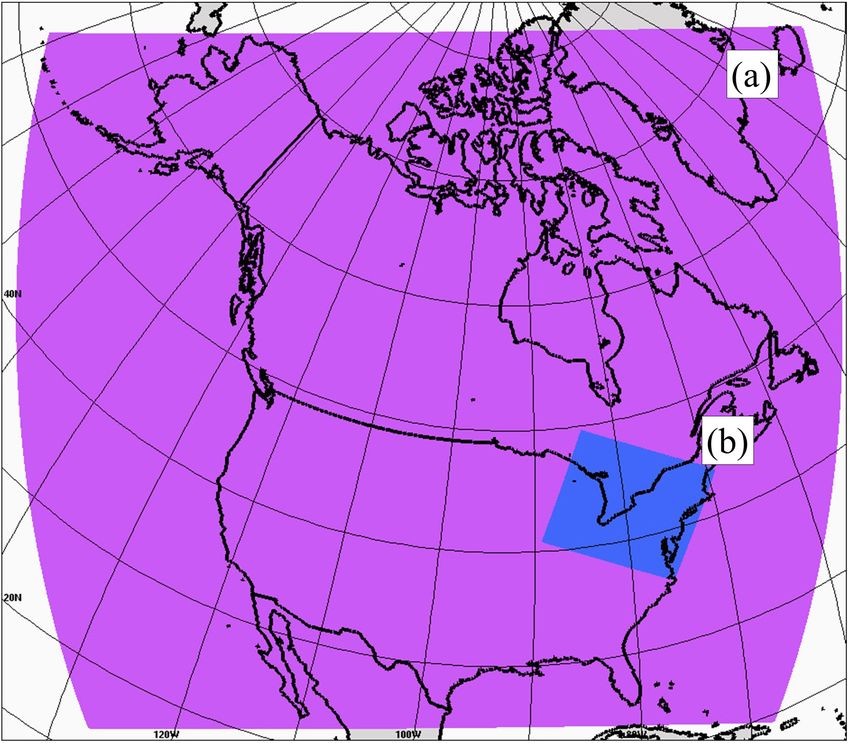
12298 P. A. Makar et al.: Vehicle-induced turbulence and atmospheric pollution
Figure 2. Illustration of the impact of VIT on the local vertical gradient of the thermal turbulent transfer coefficients, at high (a, c) and
low (b, d) resolution. Purple, green, dashed blue, and red lines illustrate the height variation in concentration, meteorological, or natural
coefficient of thermal turbulent transfer, VIT coefficient of thermal turbulent transfer, and net coefficient of thermal turbulent transfer, re-
spectively. (a, b) High- and low-resolution profiles and gradients, for the case where both concentration and meteorological thermal turbulent
transfer coefficients decrease with height. (c, d) High- and low-resolution profiles and gradients, for the case where concentration decreases
and meteorological thermal turbulent transfer coefficients increases with height.
of the TKE contributed over the larger roadways and main vertical transport due to modifications to the resolved gra-
arteries of urban areas. dient in thermal turbulent transfer coefficients, as discussed
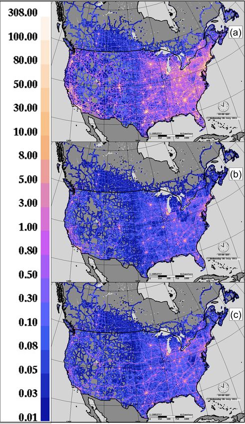
An example of the gridded vehicle-induced thermal turbu- above. Both the magnitude and gradient of Knet = K + KVIT
lent transfer coefficient values (KVIT , Eq. 8) created using may contribute to the concentration changes: breaking the
these assumptions, at 10:00 EDT, for our North American vertical diffusion equation down using the chain rule, Eq. (5)
10 km resolution domain, is shown in Fig. 4a. An an example may be rewritten as
vertical profile of KVIT for central Manhattan Island at 0.5 m
vertical resolution is shown in Fig. 4b. The resulting enhance- ∂c ∂ 2 c ∂K ∂c
=K 2 + . (9)
ments to “natural” K values at the vertical resolution of the ∂t ∂z ∂z ∂z
version of the GEM-MACH air-quality model at 2.5 km hor- Both terms on the right-hand-side of Eq. (9) may contribute
izontal resolution are shown in Fig. S1 in the Supplement as to decreases in concentration c at the surface and increases in
dashed lines. The enhancements are confined to the lowest concentrations aloft. If the near-surface concentration profile
model layer, as might be expected from the vertical resolu- (∂c/∂z) is negative (concentrations decrease with height),
tion employed in this version of GEM-MACH. Nevertheless, then increases in K will result in surface concentration de-
the values are sufficient to significantly change simulated creases). If this results in sufficient lofting that the concen-
Atmos. Chem. Phys., 21, 12291–12316, 2021 https://doi.org/10.5194/acp-21-12291-2021
P. A. Makar et al.: Vehicle-induced turbulence and atmospheric pollution                                                     12299

                                                                     are typically on the order of 0.1 to 2.0 m2 s−1 ). Aside from
                                                                     Fig. S1a, the vertical profiles here would not be modified
                                                                     by these lower limits. We also note that these VIT-induced
                                                                     changes in total thermal turbulent transfer coefficients only
                                                                     impact the species emitted at the roadway level, as discussed
                                                                     below.

                                                                     2.5   Construction of a sub-grid-scale parameterization
                                                                           for on-road vehicle-induced turbulence

                                                                     We note that the portion of the area of a grid cell which is
                                                                     roadway-covered will be relatively small for most air pol-
                                                                     lution model resolutions, such as those considered here. For
                                                                     example, satellite imagery of the largest freeways show these
                                                                     to have a width of less than 400 m. Hence, the largest roads
                                                                     make up less than 1/5 of the total area of a 2.5 km grid cell,
                                                                     and less than 1/20 of a 10 km grid cell). The largest impact
                                                                     of VIT is thus likely to be for the chemical species being
                                                                     emitted by the mobile sources, in terms of the grid cell aver-
                                                                     age concentration. Furthermore, the grid cell approach com-
                                                                     mon to these models results in horizontal numerical diffusion
                                                                     from the roadway scale to the grid cell scale: sub-grid-cell-
                                                                     scale emissions are automatically mixed across the extent of
                                                                     the grid cell. The key impact of VIT will thus be in the verti-
                                                                     cal dispersion of the pollutants emitted from mobile sources.
                                                                     We must therefore devise a numerical means to ensure this
                                                                     additional source of diffusion is added to the model, bearing
                                                                     these constraints in mind.
                                                                        Two examples of similar sub-grid-scale processes appear
                                                                     in the literature. The first example is the cloud convection
                                                                     parameterizations used in numerical weather forecast mod-
                                                                     els (Kain, 2004), wherein the formation and vertical transport
                                                                     associated with convective clouds, known to occur at smaller
Figure 3. Vehicle kilometer traveled per 10 km grid cell (km s−1 )   scales than the grid cell size employed in a numerical weather
for (a) cars, (b) mid-size vehicles, and (c) trucks, July 2015.      prediction model, are treated using sub-grid-scale parame-
                                                                     terizations. In these parameterizations, cloud formation and
                                                                     transport are calculated within the grid cell on a statistical
tration profile maximizes above the ground (i.e., (∂c)/(∂z)          basis, using formulae linking the local processes to the re-
becomes positive near the surface), then decreasing values of        solvable scale of the model. The second example is found
K with height (i.e., negative values of (∂K)/(∂z)) will also         in the treatment of emissions from large stacks within air-
result in a shift towards negative rates of change, through the      quality forecast models (Gordon et al., 2018; Akingunola et
second term in the right-hand-side of Eq. (9). All six panels        al., 2018). These sources usually have stack diameters on the
of Fig. S1 show increased Kvalues, i.e., increases in the first      order less than 10 m, and these sources emit large amounts of
term in Eq. (9). All six panels also show a trend of (∂K)/(∂z)       pollutant mass at high temperatures and velocities. In order
becoming more negative (that is, near-surface positive slopes        to represent these sources, the most common approach is to
become less positive and negative slopes become more nega-           calculate the height of the buoyant plume using the predicted
tive), decreasing the magnitude of the second term in Eq. (9)        ambient meteorology (vertical temperature profile, etc.) as
in Fig. S1b–d and f and switching to a negative rate of change       well as the stack parameters (exit velocity, exit temperature,
in Fig. S1a and e. Both changes in the magnitude and gra-            stack diameter). The emitted mass during the model time step
dient of K resulting from VIT contribute to the resulting            from the stack is then distributed over a defined vertical re-
changes in surface concentration.                                    gion within the grid cell in which the source resides. Note
   The thermal turbulent transfer coefficient values of Fig. S1      that the mass is also automatically distributed immediately in
may also be compared to the minima on natural K values               the horizontal dimension within the grid cell – the key issue
imposed in air pollution models in an attempt to account             is to ensure that the emitted mass is properly distributed in
for missing subgrid-scale mixing (Makar et al., 2014; these          the vertical dimension. Our aim in the VIT parameterization

https://doi.org/10.5194/acp-21-12291-2021                                          Atmos. Chem. Phys., 21, 12291–12316, 2021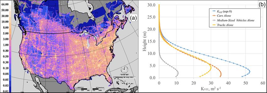
12300                                                 P. A. Makar et al.: Vehicle-induced turbulence and atmospheric pollution

Figure 4. (a) Example estimated thermal turbulent transfer coefficients from VIT at 2 m elevation during a weekday at 10:00 in July (m2 s−1 ),
using the VKT data of Fig. 3. (b) Vertical profile of VIT thermal turbulent transfer coefficients at 1 m resolution in central Manhattan Island
and individual values for the TKE associated with cars, mid-sized vehicles, and trucks considered separately, generated using Eq. (8). Note
that the profiles of (b) would be added to the ambient thermal diffusivity coefficients (see Sect. 2.5 and Eq. 12).

that follows is identical in intent to that of the existing major         by non-mobile area sources and vertical diffusion due to me-
point source treatments in air-quality models: to redistribute            teorological sources of turbulence within the grid cell but
the mass emitted by vehicle sources in the vertical dimen-                outside of the sub-grid-scale roadway. The second term de-
sion, taking the very local physics influencing that vertical             scribes the rate of change in the vertical diffusion of the
transport of fresh emissions into account. We therefore fo-               mobile-source-emitted pollutants over the sub-grid cell road-
cus on determining the at-source vertical transport of emitted            way, which experiences both meteorological and roadway
mass associated with VIT.                                                 turbulence, and the final term prevents double-counting of
   We start with the formulae for the transport of chemical               the meteorological component in Eq. (11), which is equiva-
species by vertical diffusion:                                            lent to Eq. (12). Note that turbulent mixing for non-emitted
                                                                        chemicals is determined by solving Eq. (5), and for chem-
∂ci      ∂      ∂ci
     =       K        + Ei ,                                 (10)         icals which are not emitted from mobile on-road sources,
 ∂t     ∂z      ∂z                                                        Eq. (10) is solved with Ei = Ei,oth . This form of the diffu-
where ci is the emitted chemical species, K represents the                sion Eq. (12) allows the net change in concentration to be
sum of all forms of thermal turbulent transfer in the grid cell,          calculated from three successive calls of the diffusion solver,
and Ei is the emissions source term for the species emit-                 starting from the same initial concentration field. One advan-
ted at the surface (applied as a lower boundary condition on              tage of this approach is that existing code modules for the so-
the diffusion equation). For grid cells containing roadways               lution of the vertical diffusion equation may be used – rather
and hence mobile emissions, we split K into meteorologi-                  than being used once, they are used three times, with dif-
cal and vehicle-induced components (KT and KVIT , respec-                 ferent values for the input coefficients of thermal turbulent
tively) and the emissions into those from mobile sources and              transfer coefficient (K) and for the lower boundary condi-
those from all other sources (Ei,mob and Ei,oth , respectively):          tions (E). The solution, once a suitable means of estimating
                                                                        KVIT is available, is thus relatively easy to implement in ex-
∂ci      ∂                 ∂ci                                            isting numerical air pollution model frameworks.
     =        (KT + KVIT )       + Ei,mob + Ei,oth .       (11)
 ∂t      ∂z                ∂z
The terms in Eq. (11) may be rearranged:                                  2.6   Comparison of energy densities: VIT, solar, and
                                                                            urban perturbations in sensible and latent heat
∂ci      ∂       ∂ci
    =         KT       + Ei,oth
 ∂t      ∂z      ∂z                                                       The relative contribution of TKE from VIT towards energy

           ∂                  ∂ci                                         density can be compared to the daytime solar maximum en-
       +       (KT + KVIT )         + Ei,mob                              ergy input to illustrate why VKT has relatively little impact
           ∂z                 ∂z

           ∂       ∂ci
                                                                        during daylight hours, particularly in the summer. The max-
       −       KT         .                                    (12)       imum TKE from VIT can be determined easily from Fig. 3
           ∂z      ∂z
                                                                          and the use of our formulae; Fig. 3a shows vehicle kilometer
The first bracketed term in Eq. (12) describes the rate of                traveled values ranging from a maximum of 308 in the high-
change of the chemical’s concentration due to its emission                est density 10 km grid cell in North America (New York City)

Atmos. Chem. Phys., 21, 12291–12316, 2021                                                   https://doi.org/10.5194/acp-21-12291-2021
P. A. Makar et al.: Vehicle-induced turbulence and atmospheric pollution 12301
down through 4 orders of magnitude in background grid cells ganic particle thermodynamics, secondary organic aerosol
with few vehicles. A typical urban value would be 30.8 VKT: formation, vertical diffusion (in which area sources such
this gives an Fc value from our formulae of 3.08 vehicles s−1 as vehicle emissions are treated as lower boundary condi-
for a 10 km grid cell size. Assuming that the vehicles are tions on the vertical diffusion equation), advective trans-
all cars, from our formulae we have a corresponding total port, and particle microphysics and deposition. The model
TKE added at the point crossed by the vehicles, at height makes use of a sectional approach for the aerosol size dis-
z = hcars = 1.5 m, of 7.48 m2 s−2 . We can combine this and tribution, here employing 12 aerosol bins. The version used
the Fc value along with the area and volume of a lane of here also follows the “fully coupled” paradigm – the aerosols
a roadway to estimate the energy density (EVIT ) on dimen- formed in the model’s chemical modules in turn may modify
sional grounds: the model’s meteorology via the direct and indirect effects
(Makar et al., 2015a, b, 2017). The meteorological model
(TKE) (air density) (lane volume) Fc forming the basis of the simulations carried out here is ver-
EVIT = . (13)
(lane area) sion 4.9.8 of the Global Environmental Multiscale weather
Assuming each vehicle has a length of 4.5 m, width of 2.0 m, forecast model (Cote et al., 1998a, b; Caron et al., 2015;
height of 1.5 m, a lane length of 10 km, and an air density Milbrandt et al., 2016). Emissions for the simulations con-
of 1.225 kg m−3 , one arrives at 84.8 kg s−3 and values rang- ducted here were created from the most recent available in-
ing from a North American grid maximum of 848 kg s−3 to ventories at the time the simulations were carried out – the
a background value 4 orders of magnitude smaller (8.48 × 2015 Canadian area and point source emissions inventory,
10−2 kg s−3 ). These energy densities may be compared to the 2013 Canadian transportation (on-road and off-road) emis-
typical solar energy density reaching the surface at midlati- sions inventory, and 2011-based projected 2017 US emis-
tudes of 1300 W m−2 , or in SI units, 1300 kg s−3 , and the typ- sions inventory. As noted above, the model simulations were
ical range of perturbations in latent and sensible heat fluxes carried out on two separate model domains shown in Fig. 5:
associated with the use of a more complex urban radiative a 10 km horizontal grid cell size North American domain
transfer scheme (the town energy balance module; Mason, (768 × 638 grid cells; 7680 × 6380 km) and a 2.5 km hori-
2000) in our 2.5 km grid cell size simulations (typical diur- zontal grid cell size Pan Am Games domain (520 × 420 grid
nal ranges in the perturbations associated with versus with- cells; 1300 km × 1050 km). For the 10 km domain, simula-
out the use of the town energy balance (TEB): latent, −200 tions were for the month of July 2016, while for the higher-
to +3 W m−2 ; sensible, −100 to +100 W m−2 , respectively). resolution model, month-long summer (July 2015) and win-
That is, under most daylight conditions, the energy densities ter (January 2016) simulations were carried out with and
associated with VIT will be relatively small compared to the without the VIT parameterization. These periods were based
solar energy density at midday, with a typical urban value on the availability of emissions data, previous model simu-
of 6.5 % and a range from 65 % in the cell with the high- lations for the same time periods appearing in the literature
est VKT values down to 0.0065 % in background conditions (Makar et al., 2017; Stroud et al., 2020), and the timing of a
where the vehicle numbers are relatively small. Urban traffic prior field study (Stroud et al., 2020).
however may contribute similar energy levels as the changes
in net latent and sensible heat fluxes associated with the use 2.8 VIT as a sub-grid-scale phenomena
of an urban canopy radiative transfer model. We also note
that at night, during the low sun angle conditions of early It should be noted that the VIT enhancements to turbulent
dawn and late evening and during the lower sun angles of exchange coefficients are used to determine the vertical dis-
winter, the relative importance of VIT to solar radiative in- tribution of freshly emitted pollutants at each model time
put will be larger. Consequently, the impact of VIT will be step – they are not applied for all species within a model
higher at night and in the early morning rush hours and at grid cell. Similar sub-grid-scale approaches are used for the
other times when the sun is down or sun angles are low, as is vertical redistribution of mass from large stack sources of
demonstrated below. pollutants, where buoyancy calculations are applied to de-
termine the rise and vertical distribution of pollutants from
2.7 GEM-MACH simulations large industrial sources. Both stacks and roadways are treated
as sub-grid-scale sources of pollutants which are influenced
A research version of the Global Environmental Multiscale by very local sources of energy (stacks: high emission tem-
– Modelling Air-quality and CHemistry (GEM-MACH) nu- peratures and exit velocities; roadways: vehicle-induced tur-
merical air-quality model, based on version 2.0.3 of the bulence) resulting in an enhanced vertical redistribution of
GEM-MACH platform, was used for the simulations car- newly emitted chemical species. In both cases, the vertical
ried out here (Makar et al., 2017; Moran et al., 2010, 2018; transport results from an interplay between the energy as-
Chen et al., 2020). GEM-MACH is a comprehensive 3D de- sociated with the emission process (stacks: high temperature
terministic predictive numerical transport model, with pro- emissions with the ambient vertical temperature profile; VIT:
cess modules for gas and aqueous phase chemistry, inor- kinetic energy imparted to the atmosphere in which emis-
https://doi.org/10.5194/acp-21-12291-2021 Atmos. Chem. Phys., 21, 12291–12316, 202112302 P. A. Makar et al.: Vehicle-induced turbulence and atmospheric pollution
tour plots of published data, and is subdivided into isolated
vehicle and vehicle ensemble studies and cases.
The inferred mixing length shows a marked variation be-
tween that of isolated vehicles or the lead vehicle in an en-
semble and that of other vehicles appearing further back in
the ensemble. Both directly observed and CFD modeled val-
ues of the inferred mixing length for isolated vehicles or the
lead vehicles of an ensemble vary from 2.5 to 5.13 m. For
subsequent vehicles in an ensemble, the mixing lengths in-
crease to range from 4.6 to 41 m. The difference in mixing
length between the lead vehicle in an ensemble and subse-
quent identical vehicles appearing later in the ensemble also
increases. For example note that diesel truck mixing lengths
inferred from the CFD modeling examining different vehi-
cle configurations (Y. Kim et al., 2016) increase from 5.13
to 14.64 m, and the mixing lengths for automobiles increase
from 2.50 (isolated automobile) to 4.6 (automobile two ve-
Figure 5. GEM-MACH test domains: (a) 10 km grid cell size North hicles back from a lead diesel truck) to 9.41 m (automo-
American domain; (b) 2.5 km grid cell size Pan Am domain. bile immediately behind a leading diesel truck). The mixing
length associated with VIT may also be significantly influ-
enced by the ambient wind and local built environment – the
sions have been injected with the ambient turbulent kinetic mixing length associated with the component of TKE due to
energy). This interaction precludes a treatment solely from VIT within street canyons (Woodward et al., 2019; Zhang et
the standpoint of model input emissions, since the extent al., 2017) ranges from 2/3 to greater than the street canyon
of the mixing will depend on the local atmospheric condi- height, with maximum mixing lengths of 41 m. It is impor-
tions as well as the energy added due to the manner in which tant to note that these mixing lengths are driven by the ve-
the emissions occur. Both processes have been addressed by hicle passage within the canyon; they result from the addi-
large eddy simulation modeling on a very local scale, but pa- tional TKE added due to the presence of vehicles in the CFD
rameterizations are required in both cases for regional-scale simulations. The above data show that a Gaussian distribu-
simulations. In both cases, the parameterized vertical redis- tion provides a reasonable description of the decrease in TKE
tribution of pollutants is applied to freshly emitted species from vehicles with height, and, under realistic traffic condi-
– the horizontal spatial extent of the emitting region is suf- tions, the mixing lengths increase in size and are consider-
ficiently small that although present, the enhanced mixing ably larger than those of isolated vehicles and are compara-
will have a minor effect on the redistribution of pre-existing ble to or greater than the near-surface vertical discretization
chemicals and on other atmospheric constituents affected by of air-quality models.
vertical transport. VIT in the context of regional chemical The length scales associated with VIT range from 2.50 m
transport models is thus best treated as a sub-grid-scale phe- in the case of isolated vehicles (Y. Kim et al., 2016), through
nomenon applied to fresh emissions, in direct analogy to the ∼ 10 m for vehicles moving in ensembles (Woodward et al.,
approach taken for large stack emissions. 2019; Zhang et al., 2017) up to 41 m, with the larger values
being typical for urban street canyons. The latter describe the
specific regions in which VIT is expected to have the greatest
impact, given the high vehicle density within the urban core.
3 Results However, our parameterization makes use of length scales
derived from observations on open (non-street canyon) free-
3.1 VIT height dependence as a Gaussian distribution ways (Gordon et al. 2012; Miller et al., 2018) and thus may
underestimate the length scales in the urban core. The impact
In the Methodology section, we describe the potential for the of multiple vehicles traveling in an ensemble on open road-
use of a Gaussian distribution to describe the fall-off in TKE ways was specifically depicted in the open roadway simula-
with height above vehicles. Using the equations presented tions of Y. Kim et al. (2016) reproduced in Fig. 1, where the
there, we have analyzed VIT studies appearing in the litera- vertical extent of turbulent mixing was shown to grow with
ture, determining the decrease in TKE as a function of height increasing number of vehicles traveling in an ensemble. Fur-
from published figures and then fitting these data to a Gaus- thermore, as was discussed and demonstrated in the Method-
sian distribution to the height above ground. The result of ology section using the diffusivity equation, the length scale
this analysis for several data sets is shown in Table 1, gener- of the turbulence need not be greater than the model lowest
ated by extracting vehicle centerline TKE values from con- layer resolution in order to capture the impacts of VIT on
Atmos. Chem. Phys., 21, 12291–12316, 2021 https://doi.org/10.5194/acp-21-12291-2021You can also read