Dynamics and circulation of Venus and Titan
←
→
Page content transcription
If your browser does not render page correctly, please read the page content below
ATMOSPHERIC , O CEANIC
                                     AND   P LANETARY P HYSICS
                                       U NIVERSITY OF OXFORD

          DPhil First Year Report

Dynamics and circulation of Venus and
               Titan

          João Manuel Mendonça

                    Supervisor
              Prof. Peter L. Read

                   Co-Supervisor
             Dr. Stephen R. Lewis
              (The Open University)

                   August 2009

            E-mail: Mendonca@atm.ox.ac.uk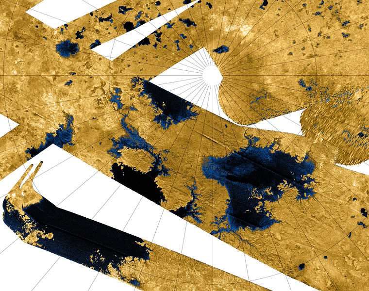
Dynamics and Circulation of Venus and Titan
Abstract:
     The main objective of my DPhil is to study and understand the atmospheric circula-
tion of slowly rotating "planets" such as Venus and Titan, that despite their differences,
exhibit a strong planetwide super-rotating zonal winds and other similar features in their
atmospheres.
     To achieve this goal, we use Simplified General Circulation Models (SGCMs) adapted
for both atmospheres. These models use simplified parameterisations as explained in Chap-
ter 4, 6 and 7. These simplifications save computational time and avoid difficulties regard-
ing the observational data about these astronomical objects, nevertheless they attempt to
keep a realistic dynamic circulation of the atmosphere, essential for our objectives.
     In the first year of my PhD project, I started by reading the literature on the subject of
General Circulation Models (GCMs) for Venus and Titan, with special emphasis on simpli-
fied models and methods to extend the SGCM for Venus improving the radiative scheme.
The new parameterisation of the radiative scheme in the SGCM for Venus, transforms the
model to a more complete version (Full GCM) which allows us to better compare the results
of the model with observational data. Amongst other features, the possible existence of a
transport barrier in the atmosphere of Venus from the analysis of potential vorticity (PV)
fields, and the possible influence of eddy momentum fluxes in the middle atmosphere near
the jets, were investigated. The basis for the first Simplified General Circulation Model
(SGCM) for Titan was developed, and has a similar structure than the one for Venus.
     This report is a description of the work done, and is structured as follows: I first write a
literature review, followed by the results of the research I have done for each Astronomical
object (Venus and Titan), and finally present a summary of my future plan of work.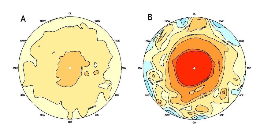
Contents

1   Introduction                                                                                                                        1
    1.1 Super-rotating Atmospheres of Venus and Titan . . . . . . . . . . . . . . .                                                     1
    1.2 Proposed Methodology . . . . . . . . . . . . . . . . . . . . . . . . . . . .                                                    2
    1.3 Report Summary . . . . . . . . . . . . . . . . . . . . . . . . . . . . . . .                                                    3

2   General Characteristics of Venus and Titan                                                                                           5
    2.1 Venus . . . . . . . . . . . . . . . . . . . . . .                   .   .   .   .   .   .   .   .   .   .   .   .   .   .   .    5
        2.1.1 Surface . . . . . . . . . . . . . . . . .                     .   .   .   .   .   .   .   .   .   .   .   .   .   .   .    8
        2.1.2 Atmospheric Composition and Clouds .                          .   .   .   .   .   .   .   .   .   .   .   .   .   .   .   10
        2.1.3 Thermal Structure and Energy Balance                          .   .   .   .   .   .   .   .   .   .   .   .   .   .   .   11
        2.1.4 Atmospheric Dynamics . . . . . . . . .                        .   .   .   .   .   .   .   .   .   .   .   .   .   .   .   12
    2.2 Titan . . . . . . . . . . . . . . . . . . . . . . .                 .   .   .   .   .   .   .   .   .   .   .   .   .   .   .   16
        2.2.1 Surface . . . . . . . . . . . . . . . . .                     .   .   .   .   .   .   .   .   .   .   .   .   .   .   .   17
        2.2.2 Atmospheric Composition and Clouds .                          .   .   .   .   .   .   .   .   .   .   .   .   .   .   .   18
        2.2.3 Thermal Structure and Energy Balance                          .   .   .   .   .   .   .   .   .   .   .   .   .   .   .   19
        2.2.4 Atmospheric Dynamics . . . . . . . . .                        .   .   .   .   .   .   .   .   .   .   .   .   .   .   .   21

3   General Circulation Models for Venus and Titan                                                                                      23
    3.1 Venus . . . . . . . . . . . . . . . . . . . . .                 .   .   .   .   .   .   .   .   .   .   .   .   .   .   .   .   23
        3.1.1 Venus GCMs . . . . . . . . . . . . .                      .   .   .   .   .   .   .   .   .   .   .   .   .   .   .   .   23
        3.1.2 Recent Venus GCMs . . . . . . . . .                       .   .   .   .   .   .   .   .   .   .   .   .   .   .   .   .   24
    3.2 Titan . . . . . . . . . . . . . . . . . . . . . .               .   .   .   .   .   .   .   .   .   .   .   .   .   .   .   .   24
        3.2.1 Titan GCMs . . . . . . . . . . . . . .                    .   .   .   .   .   .   .   .   .   .   .   .   .   .   .   .   24

4   OPUS-V                                                                                                                              27
    4.1 The Model . . . . . . . . . . . .   .   .   .   .   .   .   .   .   .   .   .   .   .   .   .   .   .   .   .   .   .   .   .   27
    4.2 Simple Parameterisation . . . .     .   .   .   .   .   .   .   .   .   .   .   .   .   .   .   .   .   .   .   .   .   .   .   29
        4.2.1 Thermal Forcing . . . .       .   .   .   .   .   .   .   .   .   .   .   .   .   .   .   .   .   .   .   .   .   .   .   29
        4.2.2 Boundary Layer Scheme         .   .   .   .   .   .   .   .   .   .   .   .   .   .   .   .   .   .   .   .   .   .   .   30

5   Research using OPUS-V                                                            31
         5.0.3 Atmospheric Transport . . . . . . . . . . . . . . . . . . . . . . . . 31
         5.0.4 Meridional Study of the Atmospheric Dynamics . . . . . . . . . . 34

6   New Radiative Scheme on OPUS-V                                                                                                      39
    6.1 Shortwaves’ Scheme . . . . . . . . . . .                .   .   .   .   .   .   .   .   .   .   .   .   .   .   .   .   .   .   39
    6.2 Longwaves’ Scheme . . . . . . . . . . .                 .   .   .   .   .   .   .   .   .   .   .   .   .   .   .   .   .   .   39
        6.2.1 The Problem . . . . . . . . . . .                 .   .   .   .   .   .   .   .   .   .   .   .   .   .   .   .   .   .   39
        6.2.2 Net-Exchange Rate Matrix . . . .                  .   .   .   .   .   .   .   .   .   .   .   .   .   .   .   .   .   .   40
        6.2.3 Adaptation of the NER Formalim                    .   .   .   .   .   .   .   .   .   .   .   .   .   .   .   .   .   .   40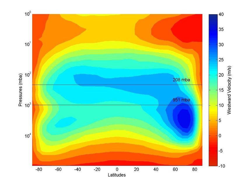
iv                                                                                                                               Contents

           6.2.4 KARINE . . . . . . . . . . . . . . . . . . . . . . .                                        .   .   .   .   .   .   .   .   41
     6.3   Results . . . . . . . . . . . . . . . . . . . . . . . . . . . . .                                 .   .   .   .   .   .   .   .   41
           6.3.1 IR Radiative Budget and Net-Exchange Rate matrix                                            .   .   .   .   .   .   .   .   41
           6.3.2 Vertical Temperature profile . . . . . . . . . . . . .                                      .   .   .   .   .   .   .   .   43

7    Preliminary Results from OPUS-T                                                                                                         45
     7.1 The Model . . . . . . . . . . .     .   .   .   .   .   .   .   .   .   .   .   .   .   .   .   .   .   .   .   .   .   .   .   .   45
     7.2 Simple Parameterisations . . .      .   .   .   .   .   .   .   .   .   .   .   .   .   .   .   .   .   .   .   .   .   .   .   .   46
          7.2.1 Basic Parameters . . .       .   .   .   .   .   .   .   .   .   .   .   .   .   .   .   .   .   .   .   .   .   .   .   .   46
          7.2.2 Radiative Forcing . . .      .   .   .   .   .   .   .   .   .   .   .   .   .   .   .   .   .   .   .   .   .   .   .   .   46
     7.3 Spin-up Phase . . . . . . . . .     .   .   .   .   .   .   .   .   .   .   .   .   .   .   .   .   .   .   .   .   .   .   .   .   50

8    Conclusions and Future Work                                                         55
     8.1 Conclusions . . . . . . . . . . . . . . . . . . . . . . . . . . . . . . . . . . 55
     8.2 Future Work . . . . . . . . . . . . . . . . . . . . . . . . . . . . . . . . . . 56
     8.3 Approximate Timeline . . . . . . . . . . . . . . . . . . . . . . . . . . . . 57

A Basic Equations                                                                     59
  A.1 Primitive Equations . . . . . . . . . . . . . . . . . . . . . . . . . . . . . . 59
  A.2 The Eulerian-Mean Equations . . . . . . . . . . . . . . . . . . . . . . . . 60

Bibliography                                                                                                                                 61
List of Figures
2.1 UV image of Venus’ clouds. . . . . . . . . . . . . . . . . . . . . . . . . . 6
2.2 Surface of Venus measured by Magellan probe (1990’s) . . . . . . . . . . . 8
2.3 Nightside of Venus in the near-infrared ’window’ at 2.3 µm. . . . . . . . . 11
2.4 Reflected solar flux and thermal flux, in Earth and Venus. . . . . . . . . . . 12
2.5 Temperature profiles in Venus. . . . . . . . . . . . . . . . . . . . . . . . . 13
2.6 Scheme of the main features of the atmospheric circulation on Venus. . . . 13
2.7 Venus wind profiles (Height-Wind velocity) from the Pioneer Probes. . . . 14
2.8 The North polar vortex from Mariner 10 and Pioneer Venus Orbiter (Taylor,
2006). . . . . . . . . . . . . . . . . . . . . . . . . . . . . . . . . . . . . . 15
2.9 Summary of vertical structure of Titan’s atmosphere. . . . . . . . . . . . . 16
2.10 Radar images to date of Titan’s north polar region. . . . . . . . . . . . . . . 17
2.11 Reference temperature profile used in the thermal forcing for Titan GCM. . 19
2.12 Schematic Titan’s general circulation for the northern spring. . . . . . . . . 21
2.13 Zonal wind profile obtained by Huygens probe. . . . . . . . . . . . . . . . 21
4.1 Prognostic variables diagnostics of the Oxford Venus GCM. . . . . . . . . 28
4.2 Equatorial Kelvin and Mixed Rossby Gravity Waves from Lee (2006) . . . 29
5.1 PV fields from Mars and Earth. . . . . . . . . . . . . . . . . . . . . . . . . 32
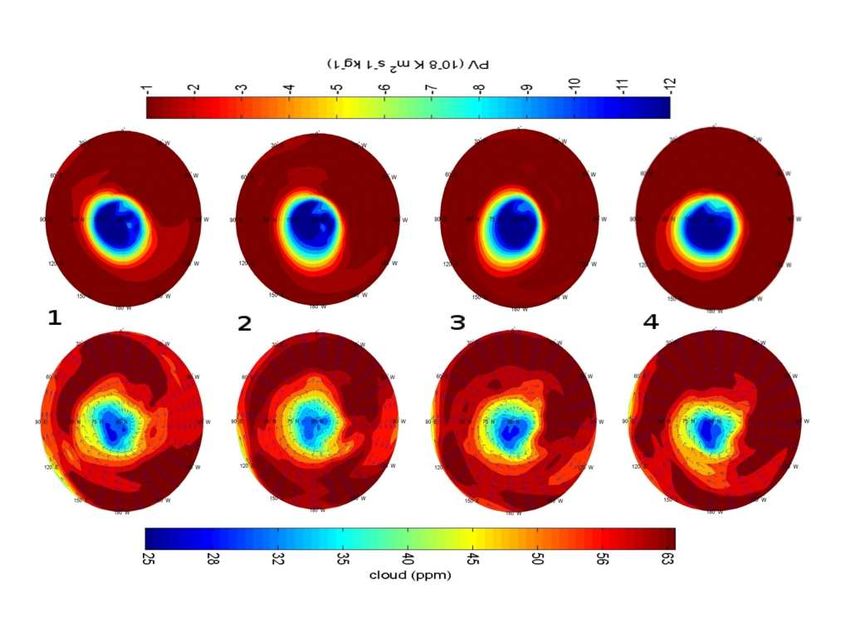
5.2 PV field and cloud distribution at the Polar vortex. . . . . . . . . . . . . . . 32
5.3 Zonal and time cloud liquid concentration. . . . . . . . . . . . . . . . . . . 33
5.4 Zonal thermal wind speed from cyclostrophic approximation. . . . . . . . . 34
5.5 Evaluation of each term of the meridional component of the equation of
motion. . . . . . . . . . . . . . . . . . . . . . . . . . . . . . . . . . . . . 36
5.6 Eddy forcing terms. . . . . . . . . . . . . . . . . . . . . . . . . . . . . . . 37
5.7 Evaluation of each term of the meridional component of the equation of
motion including eddy forcing terms. . . . . . . . . . . . . . . . . . . . . . 38
6.1 Radiative budget and spectrally integrated Net Exchange Rate matrix for
the thermal radiation and the temperature profiles. . . . . . . . . . . . . . . 42
7.1 Zonal mean relaxation temperature fields for two different declination angles. 49
7.2 The "hotspot" used for the diurnal and seasonal forcing. . . . . . . . . . . . 49
7.3 Longitudinally averaged westward wind speed (m s−1 ) during the spin-up
phase. . . . . . . . . . . . . . . . . . . . . . . . . . . . . . . . . . . . . . 50
7.4 Prognostic variables diagnostics of the Oxford Titan GCM. . . . . . . . . . 52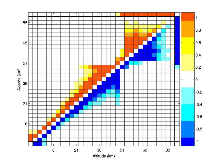
List of Tables

2.1   Table from Lee (2006) with the bulk, orbital and atmospheric parameters
      for Venus. . . . . . . . . . . . . . . . . . . . . . . . . . . . . . . . . . .   . 9
2.2   Venus atmospheric composition . . . . . . . . . . . . . . . . . . . . . .        . 10
2.3   Atmospheric Composition of Titan. . . . . . . . . . . . . . . . . . . . .        . 18
2.4   Titan atmospheric’s properties from Atreya (1986). . . . . . . . . . . . .       . 20

7.1   Values used in the Titan GCM. . . . . . . . . . . . . . . . . . . . . . . . . 48

8.1   Future Work Timeline . . . . . . . . . . . . . . . . . . . . . . . . . . . . . 57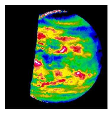
C HAPTER 1

                                                                Introduction

Contents
        1.1   Super-rotating Atmospheres of Venus and Titan . . . . . . . . . . . . .      1
        1.2   Proposed Methodology . . . . . . . . . . . . . . . . . . . . . . . . . . .   2
        1.3   Report Summary . . . . . . . . . . . . . . . . . . . . . . . . . . . . . .   3

1.1      Super-rotating Atmospheres of Venus and Titan
The circulation of the atmospheres of both Venus and Titan are well known to exhibit
strong super-rotation and a variety of similar enigmatic features, but both remain poorly
understood (see Chapter 2). The super-rotation is characterised by a faster rotation of the
atmosphere compared to the rotation rate of the solid body, and is most likely found in
slowly rotating "telluric bodies". This is a surprising phenomenon because it is counter
intuitive if we think on results of solid bodies in a regime of no rotation. Having a better
understanding of the mechanism of formation and maintenance of this phenomenon, we
can draw a more accurate theory about the global circulation of both atmospheres.
    When studying the circulation of Venus and Titan’s atmospheres, some general ques-
tions arise about their super-rotation:

      • What is the mechanism that drives these slow rotating "planets" to an atmospheric
        super-rotation?

      • Is the super-rotation an inevitable state of slow rotating "planets"?

      • What are the atmospheric and slow body’s parameters for which the atmosphere is
        sensitive to in its transition to super-rotation?

      • Are the phenomena such as the polar vortex or the large-scale wave patterns ob-
        served in the atmosphere of Venus, common in the super-rotating atmospheres?

     This DPhil investigates mainly the atmospheric circulation of two "worlds": Venus and
Titan. Despite the differences in the physical body, different rates of vertical and horizontal
profiles for heating and cooling (Venus: important diurnal variations; Titan: important
seasonal variations) and the amount of total atmospheric mass, both rotate slowly and have
a very efficient way of retaining IR radiation in the atmosphere, which increases the vertical
static stability of the atmosphere. Here we investigate the mechanism and the consequences
2 Chapter 1. Introduction
in the dynamics of the atmosphere produced by the atmospheric circulations in these two
"planets".
The aim of the comparative study about both atmospheres is to understand a variety of
atmospheric phenomena governed by common physical laws. Understand why Titan and
Venus atmospheric’s circulation produce similar phenomena, could help to answer some
key scientific questions about the atmospheric super-rotation, that will be explored in my
PhD project:
• Which types of waves are most important for sustaining super-rotation? - Planetary
waves, Gravity waves or Thermal tides?
• What is the role of topography and surface interactions?
• What is the role of seasonal variations? - Much larger on Titan than on Venus.
• What is the dynamic role of clouds either as passive or active factors? Also what
determines distribution and properties of clouds across the planet? The model used
in this work (Lee et al., 2009), obtains a cloud distribution similar to observations.
1.2 Proposed Methodology
An essential tool used in my DPhil project is a numerical simulation of the atmospheric
circulation with General Circulation Models (GCMs). These models have been very im-
portant in investigating the climate and weather forecasting on Earth as well. Changing
the general parameters that characterise the planets, it is possible to adapt the model which
solves the primitive equations using for example a discretisized finite difference scheme
(the one used in our project). It is possible to modify the physical parameterisation as
well, to better adapt the planet atmosphere in study and solve problems regarding time
spent in computation. The dynamical part of the GCM usually remains the same due to
the universal laws of fluids in the atmosphere, but can be modified, as will be discussed in
Chapter 8, where we propose to include vertical variations of the specific heat. The basic
model used in this project is the "Unified Model" from the United Kingdom Meteorologi-
cal Office (version 4.5.1), which is used mainly for Earth climate research and for weather
forecasting.
The main challenge in my DPhil project is to simulate the atmospheric super-rotation
for slowly rotating "worlds" such as Venus and Titan, and have a better understanding of
the phenomenon, as said above. The circulation of these atmospheres have been studied by
several models, Chapter 3, but is still not fully understood.
The super-rotation for the upper atmosphere for both Titan and Venus, amongst several
hypothesis, is expected to follow the GRW theory where the super-rotation is caused by
a net upward transport of angular momentum by Hadley-like circulation, with large scale
barotropic eddies being the main transporter of momentum towards the equator (Gierasch
(1975) and Rossow and Williams (1979)).
Recent work in Oxford has resulted in the development of a simplified general circu-
lation model (SGCM) of the Venus atmosphere, which is already capable of quantitatively1.3. Report Summary 3
reproducing some aspects of its meteorology (Lee, 2006). We now plan to develop a more
complete GCM for the atmosphere of Venus. Amongst some modifications proposed in the
project for the Oxford Venus GCM, we are implementing a new radiative scheme based
in Net-Exchange rates matrix for the IR and table values for short-waves (see Chapter 6).
The validation of the results will be done with observational data from Venus Express for
Venus, and also from other results from successful GCMs. This Full GCM will allow a
more careful study of the role of the clouds in the circulation of Venus atmosphere and its
distribution.
The Simplified General Circulation Models (SGCMs) do not try to use fully Physics-
base representations of all physical process. However, they are very useful tools in compar-
ative studies of the different atmospheric circulations, since it is easier to adapt the model
to different conditions and where the aim is more concerned with the dynamic features of
the atmosphere. Adapting the well established Venus SGCM from Lee et al. (2007) for
Titan’s conditions, enables us to do comparative simulations and explore possible roles
for waves and seasons in simplified forms. This will improve our tools to understand the
atmospheric’s circulation, and phenomena such as the super-rotation.
1.3 Report Summary
In the next Chapter, I will give an overview of the general characteristics for Venus and
Titan namely the bulk and orbital parameters, surface, atmospheric composition and clouds,
thermal structure and energy balance, and especially atmospheric dynamics.
Chapter 3 describes the state of the art regarding general circulation models for Venus
and Titan.
On Chapter 4 the previous model developed for Venus is presented and on Chapter 5
new diagnostics are computed to study mixing barriers and the importance of eddy mo-
mentum fluxes in the upper atmosphere on this model.
Chapter 6 outlines the new radiative scheme which is being implemented in the Venus
GCM and shows some diagnostics with that new parameterisation.
Chapter 7 presents the new Oxford Titan GCM, which has similar structure to the
previous Venus GCM developed in Oxford in 2006. It shows some results from its early
spin-up phase.
A general conclusion of my first year and a brief summary about my future work are
presented in Chapter 8.C HAPTER 2
General Characteristics of Venus
and Titan
Contents
2.1 Venus . . . . . . . . . . . . . . . . . . . . . . . . . . . . . . . . . . . . . 5
2.1.1 Surface . . . . . . . . . . . . . . . . . . . . . . . . . . . . . . . . 8
2.1.2 Atmospheric Composition and Clouds . . . . . . . . . . . . . . . . 10
2.1.3 Thermal Structure and Energy Balance . . . . . . . . . . . . . . . 11
2.1.4 Atmospheric Dynamics . . . . . . . . . . . . . . . . . . . . . . . . 12
2.2 Titan . . . . . . . . . . . . . . . . . . . . . . . . . . . . . . . . . . . . . 16
2.2.1 Surface . . . . . . . . . . . . . . . . . . . . . . . . . . . . . . . . 17
2.2.2 Atmospheric Composition and Clouds . . . . . . . . . . . . . . . . 18
2.2.3 Thermal Structure and Energy Balance . . . . . . . . . . . . . . . 19
2.2.4 Atmospheric Dynamics . . . . . . . . . . . . . . . . . . . . . . . . 21
2.1 Venus
Venus is the second closest planet to the Sun, has no moons, and it is the most Earth-
like astronomical object in our solar system (see Table 2.1). Despite this similarity, Earth
and Venus have very distinct characteristics. To explain this, if we assume that at their
formation the composition was the same, they must have had a different evolution. The
physical mechanism by which Venus evolved still remains poorly understood.
Galileo Galilei observed Venus for the first time using a telescope in 1609, and later
on, in 1631, Johannes Kepler mapped its orbit around the sun and observed the first transit
of Venus. These were early discoveries about the planet that hid its rotation velocity in
the dense layers of its atmosphere for more than 200 years. The first attempts to calculate
the rotation velocity were made by Jean-Dominique Cassini between 1666 and 1667 and
suggested a period of less than one Earth day from the observations of bright areas in
the Venus atmosphere. Several scientists tried in the 18th and 19th century to obtain an
accurate result for the Venus rotation period, but these measurements had difficulties such
as: finding points of reference in the planet and short period of time to observe Venus
from the telescopes. All the results obtained a rotation for Venus around 24h, but the
observations from 1877 to 1878 by Giovanni Virginio Schiaparelli did not show any signal6 Chapter 2. General Characteristics of Venus and Titan
Figure 2.1: Ultraviolet image of Venus’ clouds obtained by the Pioneer Venus Orbiter (Feb.
26, 1979).
of variation related with rotation. Based on its results Giovanni suggested that the rotation
was synchronised with the movement around the sun, 224.7 days. This idea was against the
value of a period of rotation of 24h shared by several scientist of his time. The true value
was only found in the 20th century, using radar measurements which allows the radiation
to penetrate in the thick atmosphere and have more accurate results for the rotation of the
planet. The observations in 1962 by the Jet Propulsion Laboratory (NASA, EUA) obtained
surprisingly a rotation in the inverse direction and very slow, with a period of 240.0 days
(Goldstein (1964) and Carpenter (1964)). Combining the period of rotation with the orbital
period of 224.7 days, one get a Solar day on Venus of 116 days, with the Sun rising in the
west and setting in the east.
Understanding the origin of the mysterious retrograde rotation, opposite to most of the
other bodies in the Solar System, has been a challenging problem. In Correia and Laskar
(2001), it is explained that the actual state of the retrograde rotation of Venus is not from
primordial origin (in the formation planet/solar system), but from the post-formation dy-
namical evolution. The inclination of the rotation axis of the interior planets is a degree of
freedom with irregular movement due to the coupling of rotation itself, with perturbations
due to the movement of other bodies in the solar system.
The slow retrograde rotation coupled with an orbit of eccentricity almost zero and a
low spin axis inclination leads to a very weak seasonal variation on Venus.
Despite being called Earth’s "sister planet", because of the similar size, gravity, and
bulk composition, Venus has the most massive atmosphere of the terrestrial planets, cov-
ered by an opaque layer of highly reflective clouds preventing its surface from being seen
from space in visible wavelengths. The main gas of its atmosphere is CO2 . In the Earth this
gas can be efficiently removed from the atmosphere dissolving into oceans, but in Venus
it is the major cause for the high temperature in the atmosphere and surface. CO2 as a2.1. Venus 7 "greenhouse" gas and being the main component of the atmosphere (Venus contains a to- tal of about 92 bars of CO2 ), raises the surface temperature to about 750 K, three times higher than if this effect did not exist in Venus. The clouds mainly composed by droplets of sulphuric acid have a total mass relatively small but enough to contribute to the planet’s visible appearance (see Figure 2.1), atmospheric thermal structure and energy balance.
8                               Chapter 2. General Characteristics of Venus and Titan

Figure 2.2: Radar map of the surface of Venus measured by Magellan probe (1990’s). The
red colour represents the highest levels and blue the depressions. The north pole is at the
center of the image.

2.1.1   Surface

The first estimate of the temperature on the Venus’s surface was in the 1950’s, with the pos-
sibility to measure the intensity of the microwave radiation coming from the planet using
radio telescopes. The value obtained was around 673 K, and it was confirm by the probe
Mariner 2, that showed the surface as the source of this radiation. Later, the Venera lan-
ders measured a temperature of roughly 730 K, showing a sterile, mainly basaltic, surface
like a scorched desert dominated by a rock-strewn landscape. Some questions related to
the composition, the transformations that the rocks suffer in the surface and the process of
erosion still remain unanswered.

    The satellite Magellan mapped the planet’s surface from orbit and showed that the
planet Venus is 70% covered by smoothly (rolling) plains, 20% of low lands and the last
10% highland regions, see Figure 2.2. Apparently the movement of tectonic plates seems
to not exist, and the cause of the formation of highlands, which appear as massive local
mountains, is suggested to be caused by a deep process within the crust, like a vigorous
convection in a large "hot spot" in that zone. Much of Venus’s surface appears to have been
shaped by volcanic activity. This "renews" the surface, making it look relatively young.
The several hundred craters in the surface are uniformly distributed and in a well-preserved
condition (an indication for the resurfacing phenomenon). The size of the craters is related
with the filtering of the huge atmosphere that covers the planet, which does not allow the
formation of small meteoric craters.
2.1. Venus 9
Venus Titan Earth
Mean Radius (km) 6051.8 2575.0 6371.0
Surface gravity (equator ms−2 ) 8.87 1.35 9.78
Bond Albedo 0.75 0.2 0.306
Solar Irradiance (Ws−2 ) 2623.9 14.90 1367.6
Black-body temperature (K) 231.7 84.5 254.3
Sidereal orbit period (days) 224.701 (15.95) 365.256
Tropical orbit period (days) 224.695 (15.95) 365.242
Orbit inclination (deg) 3.39 27 (relative to Saturn) 0.0
Orbit eccentricity 0.0067 0.029 0.0167
Sidereal rotation period (hrs) (-)5832.5 382.68 23.9345
(Solar) Length of day (hrs) 2802.0 383.68 24.0
Solar day / Sidereal day 0.480411 (1.000) 1.000274
Obliquity of orbit (deg) 177.36 23.45
Surface Pressure (atm) 92 1.5 1
Mean molecular weight (g/mole) 43.45 28 28.97
Gas constant (J/K/kg) 188 290 287
Specific heat (J/K/kg) 850.1 1005 1005
κ=R/Cp 0.222 0.277 0.286
Atmospheric composition 0.95 CO2 0.9-0.97 N2 0.78 N2
0.035 N2 0.201 O2
Global Super-rotation 10 6-10 0.015
Local super-rotation (maximum) 60 3-8
Sidereal day (Earth days) 243 1.025 1
Solar Days (Earth days) 116.95 1.027 1.000274
Surface Temperature (approx K) 730 94 285
Table 2.1: Table from Lee (2006) with the bulk, orbital and atmospheric parameters for
Venus (Williams, 2003), Earth (Williams, 2003) and Titan (Coustenis and Taylor (1999)
and Allison and Travis (1985)).10 Chapter 2. General Characteristics of Venus and Titan
Total mass of atmosphere 4.8×10²⁰ kg
Mean molecular weight 43.45 g/mol
Scale height 15.9km
Atmospheric composition (near surface,
by volume)
Major Carbon dioxide (CO2 ) 96.5%
Nitrogen (N2 ) 3.5%
Minor (ppm) Sulphur dioxide (SO2 ) 150
Argon (Ar) 70
Water (H2 O) 20
Carbon monoxide (CO) 17
Helium (He) 12
Neon (Ne) 7
Table 2.2: Venus atmospheric composition (Taylor, 2006)
2.1.2 Atmospheric Composition and Clouds
Venus has a dense atmosphere mainly composed of Carbon dioxide (∼96.5%) and a small
amount of nitrogen (∼3.5%), Table 2.2. It is observed in the atmosphere that some times,
the minor constituents like sulphur dioxide, carbon monoxide and water, exhibit local con-
centrations with temporal and spatial variations, which are linked with its atmospheric
circulation and meteorology, and/or some occurrence in the surface like volcanism. The
images in the UV (see Figure 2.1), show a dominant pattern in the atmosphere with the
shape of the letter "Y" or the inverse "C", laid sideways. This feature is related with some
unknown UV absorbent substances that are redistributed spatially by the dynamics on the
atmosphere.
The main cloud deck is composed mostly by sulphur dioxide and sulphuric acid droplets
and it extends from about 45 to 65 km above the surface, with haze layers above and below.
At the UV, visible and most of the infrared wavelength range, the clouds are very thick, hid-
ing completely the surface of the planet. The clouds have particles of three different modes
whose proportions are different in the different layers, with sizes ranging from less than 1
to over 30 µm in diameter. The smaller particles, ’mode 1’ droplets, extend throughout the
top of the clouds and their composition is still unknown. The droplets of the ’mode 2’ are
mainly H2 SO4 and H2 O, and the ’mode 3’ are probably composed by "bigger droplets"
of H2 SO4 and are located at lower and mid cloud layers.
The clouds have a very high optical depth and a high single scattering albedo in some
of the most significant spectral intervals, but they are not completely opaque to all wave-
lengths: some visible and near-IR spectral windows can be observed.
From the near-IR mapping spectrometer (see Figure 2.3), it is possible to observe vari-
ability on the horizontal and vertical structure of the clouds, which is a consequence of the
dynamical transport and the production and destruction of particles in the clouds.2.1. Venus 11
Figure 2.3: This false colour image is from the night side of Venus in the near-infrared
’window’ at 2.3 µm, and was obtained by the NIMS aboard the Galileo spacecraft during
its flyby in February 1990 (Carlson et al., 1991). The variations (more than one order of
magnitude) in brightness show the change in thickness of the clouds from white and red
(thin cloud regions) to black and blue (thick clouds).
2.1.3 Thermal Structure and Energy Balance
In the case of planets without an internal source of energy, the Sun is the main source of
energy. If Venus was an airless planet with an albedo of 0.76 and having the same distance
from the sun, the expected value for the surface temperature would be around 230K, which
is very different from the value observed. One possible cause for the discrepancy in the
values is related with the composition of the massive atmosphere in Venus that creates a
significant greenhouse effect. This feature is responsible for the high temperatures at the
surface. The lower atmosphere (troposphere), due to the large opacity of the overlying
layers, does not radiate enough energy at long thermal wavelength to space. It re-emits
part of the energy received back to the surface, raising its expected temperature (to around
730K).
The atmosphere of Venus is more efficient transporting heat from the equator to the
poles than the planet Earth. This feature has influence in the gradient of the net thermal
emission that is stronger in Venus (see Figure 2.4) due to the high thermal capacity and to
the more "organised" atmosphere in a less turbulent regime.
The clouds have a very important role in the thermal structure of the atmosphere since
it absorbs and reflects the major part of the solar flux radiation and contributes as well for
the "greenhouse" effect. Due to the highly reflective properties of the clouds, the planet
receives less total solar energy than the Earth.
Computing the height and the density from the accelerometer measurements of the Pi-
oneer Venus entry probe,the values of different temperature profiles for different locations
were retrieved from the hydrostatic equation complemented with the equation of state. In12 Chapter 2. General Characteristics of Venus and Titan
Figure 2.4: The purple lines represent reflected solar flux and the red lines the thermal flux
in Earth and Venus. Image from Crisp (2007).
Figure 2.5, four vertical profiles of temperature are shown (Seiff et al., 1980), plus one that
was used in the thermal forcing of the Oxford Venus GCM (Lee, 2006). The radiative time
scales which are needed as well in the parameterisation can be calculated using radiative
models (Pollack and Young, 1975). However, the values used in the GCM are less than the
values obtained for almost every altitude. This difference is mainly related to computation
cost and an advection mechanism that was neglected in the radiative calculations in Pollack
and Young (1975).
2.1.4 Atmospheric Dynamics
The circulation of the atmosphere in Venus (see Figure 2.6) is governed by two regimes
for different structures in the atmosphere: the retrograde zonal super-rotation in the tro-
posphere and mesosphere (Gierasch et al., 1997), and the solar-antisolar circulation across
the terminator in the thermosphere (Bougher et al., 1997). Several observations done by
descent probes, Vega balloons or using cloud tracking in the UV, showed that in the tro-
posphere (0 to around 70km), the winds reach a maximum of 100ms−1 at the cloud tops
and decreasing to roughly zero at the surface (Figure 2.7). In average, the main cloud deck
rotates around the planet in a period of 4-5 days, being around 50-60 times faster than
the rotation of the slowly solid body, maximum of 2ms−1 at the equator relative to the
background stars.
The dynamics of the atmosphere in Venus is driven by a differential insulation in lat-2.1. Venus 13 Figure 2.5: The black line is the temperature profile used in the thermal forcing of the Venus GCM (Lee et al., 2007). The figure was obtained from Lee (2006) which used the data from Pioneer Venus descent probe (Seiff et al., 1980). The night probe measured the temperatures up to 65 km only. The four probes obtained the data from different latitudes and local times: Sounder - 4.4◦ N, 7:38 am; Day - 32.1◦ S, 6:46 am; Night - 28.7◦ S, 0:07 am; North - 59.3◦ N, 3:35 am. Figure 2.6: The figure summarises schematically the main features of the atmospheric circulation on Venus and some questions that remain poorly understood (Taylor, 2006).
14                              Chapter 2. General Characteristics of Venus and Titan

Figure 2.7: Venus wind profiles (Height-Wind velocity) from the Pioneer Probes (Taylor,
2006).

itude, and the presence of middle or high latitude super-rotation is well explained as a
consequence of poleward angular momentum transport by a thermally direct Hadley circu-
lation. More difficult to explain, is the presence of the observed equatorial super-rotation
in its atmosphere. Such a phenomenon requires the presence of nonaxisymmetric eddy
motions, because the flow in this zone rotates with much higher angular velocity than
the one driven by a differential insulation planetary rotation under just the existence of
axisymmetric circulation, unless super-rotation was its initial condition. There are sev-
eral mechanisms that can explain the formation of such eddies: barotropic instability of a
high-latitude jet produced by the Hadley cell (Gierasch (1975) and Rossow and Williams
(1979)); transient or topographically forced planetary or small-scale gravity waves (Leovy,
1973); Solar semidiurnal thermal tide (Fels and Lindzen, 1974); and external torques (Gold
and Soter, 1971).
     The observations in the IR made by Venus Express showed a bright south pole sur-
rounded by a cold "collar" (Piccioni et al., 2007), that is very similar to what was observed
in previous missions to the north pole (Taylor et al., 1979) (see Figure 2.8). These huge
cyclonic structures change their central morphology continually, showing a single, dou-
ble or tri-pole structure that rotates around the pole. Analysing in altitude, there are two
phases that characterise the polar vortex: at about 50 km, a cold "collar" circulating around
a higher temperature polar cap, and at about 90 km, the warm pole, where the temperature
of the pole is higher than the equatorial one.
     The nature and mechanisms of the polar temperature structures and the polar vortices
are still not clear. It has been proposed that the polar temperature structures are a result
of the compressional adiabatic warming from the descending branch of the meridional
cell circulation, coupled with variations in the solar heating, due to variations in the haze
2.1. Venus 15
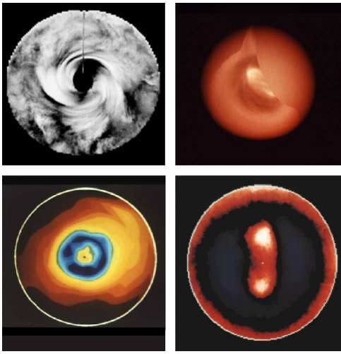
Figure 2.8: The figure shows four images of the North polar vortex (Taylor, 2006). The one
in the top left, is a UV image from Marine 10, the bottom left one was taken at 11.5 µm
with Pioneer Venus and shows the cold "collar" (Taylor et al., 1980). The top right image is
averaged over 72 days, and shows the dipole structure surrounded by a cold "collar". The
last image is about the collar-dipole structure again, which remains poorly understood.
densities at 80 km. The dynamics of the polar vortices in Venus seems to be related to the
possibility of barotropic instabilities in the polar flow (Limaye et al., 2009).
The global waves activity in Venus’ atmosphere is likely to play an important role
in the transport of momentum and energy in the atmosphere. The planetary-scale cloud
patterns observed in the UV measurements, with a shape of a large horizontal "Y", can
be explained by the presence of atmospheric waves travelling slowly with respect to the
cloud-top winds. The combination of mid latitude waves travelling somewhat slower than
the winds, interfering with slightly faster equatorial waves coupled with some non-linear
effects can explain the pattern observed. The real nature of the waves in the atmosphere of
Venus is difficult to explain due to the lack of observational data. del Genio and Rossow
(1990) studied the images from UV to study the characteristics of the waves in the atmo-
sphere of Venus, and correlated the contrasts of an unknown absorber ("Y" and reversed
"C" shape), the winds and the temperature fields. The waves observed at 65-70 km of al-
titude were of two types: equatorially trapped waves moving in the same direction as the
wind but faster, extending from its equator to roughly 20◦ latitude and with a period of 4
days, identified as a Kelvin wave; mid-latitude waves moving in the same direction of the
winds but slower, with two different periods of 4 and 5.2 days, which were intrepreted as
Mixed-Rossby-Gravity waves (del Genio and Rossow, 1990).16 Chapter 2. General Characteristics of Venus and Titan
Figure 2.9: The figure shows schematically some features of Titan’s atmosphere such as
the temperature, clouds, hazes, precipitation, surface, and radiation fluxes. This figure is
taken from Coustenis and Taylor (1999). The smooth temperature profile curve is from a
theoretical model done before the Cassini mission (Yelle et al., 1997), and the Huygens
temperature profile is from Fulchignoni et al. (2005).
2.2 Titan
In 1655 the Dutch astronomer Christian Huygens discovered the first known moon of Sat-
urn, Titan (see Table 2.1). Titan is the largest moon of Saturn, and the only moon in the
Solar System to have a thick atmosphere, which caused an overestimation in measuring its
dimensions before the arrival of Voyager 1 in 1980. It is a cold world (surface temperature
is around 94 K) covered by an atmosphere mainly composed by nitrogen, like the Earth,
but having methane as other of the main constituents, Figure 2.9.
As the Earth’s moon, Titan is tidally locked in synchronous rotation with a planet,
orbiting once every 15.94 days in a positive direction at a distance of about 1.2 million
kilometres. A small satellite called Hyperion, is locked in a 3:4 resonance with Titan,
which could have been captured by the moon from a possible chaotic trajectory.
The moon has an equatorial radius of 2575km, which makes Titan the second largest
in our solar system (Jupiter’s moon Ganymede is 112km larger). The value of the mean
density is around 1.88 g/cm3 suggesting that the composition of Titan is half water and half
rocky material compressed due to gravitation.2.2. Titan 17
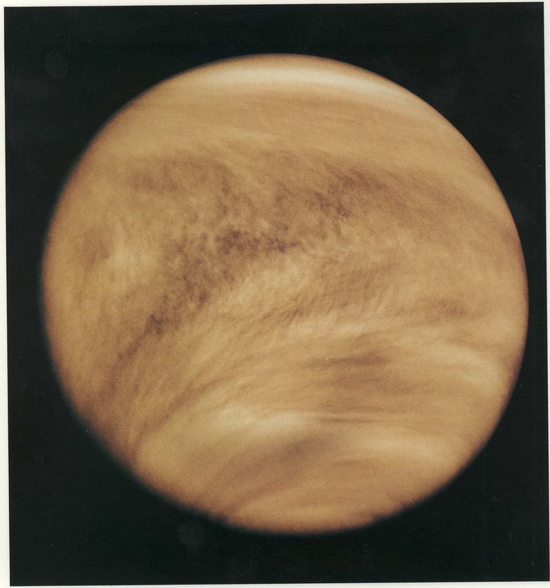
Figure 2.10: This figure shows a Cassini false-color mosaic with all synthetic-aperture
radar images to date of Titan’s north polar region. The regions with the colours in blue and
black are related with liquids (hydrocarbon lakes).
Copyright NASA/JPL/USGS
2.2.1 Surface
The satellite Cassini, which was prepared to float in hydro-carbonates like methane and
ethane because it was thought that the surface was almost completely or fully covered by
an ocean. After its launch other reality started to become more plausible, with a surface
with little or no liquid. Later, after the arrival of Cassini and the landing of Huygens, it was
discovered that the surface of Titan was in an intermediate state due to the observation of
geological structures related with the presence of liquids, like rivers and lakes of methane
and ethane (Stofan et al., 2007) (see Figure 2.10). The confirmation arrived on June 2008
with the data from Cassini’s Visible and IR Mapping Spectrometer (VIMS) about a liquid
in a Lake Ontario in Titan’s southern hemisphere (Brown et al., 2008).
The surface of Titan is relatively smooth, the observations obtain roughly height vari-
ations of the order of 150 m and the mountains have less than 2 km. The small number of
craters suggests a relatively young surface influenced by geological processes like: erosion
by winds, slushy volcanoes, as well as hydrocarbon rain and soot, depositing possibly new
material on the surface. Other feature of the moon that certainly is reducing the number of
craters is its massive atmosphere, that acts as a shield. It was estimated that the number of
craters is reduced by a factor of two due to atmospheric shielding (Ivanov et al., 1997).
There is some evidences of volcanic activity (cryovolcanism) in Titan. The cryovolcan-
ism, which is suspected to exist in Titan and highly possible to exist in many other frozen
bodies in the solar system, consists in a volcanic process involving icy fluids (water in Ti-
tan’s case), or cryolavas that is water or water-ammonia, which behave similarly to basaltic
lavas on Earth. This phenomenon, that can be a source of methane in the atmosphere, needs
heat to activate. There are some suggestions for the origin of the heat source, for example,
the decay of radioactive elements within the mantle.18 Chapter 2. General Characteristics of Venus and Titan
Constituent Mole Fraction
Major
Molecular nitrogen, N2 0.98–0.82
Methane, CH4 2×10⁻² (at 100 mb)
(8±3)×10−2 (at 3700 km)
Minor
Argon, AR362.2. Titan 19
Figure 2.11: Reference temperature profile used in the thermal forcing for Titan GCM
derived from observational data (Lindal et al., 1983).
2.2.3 Thermal Structure and Energy Balance
The cold moon of Saturn, Titan, absorbs the major part, ∼60%, of the incident solar en-
ergy before it arrives at the surface, and ∼30% is reflected back to space. The high levels
of Titan’s atmosphere absorb mainly the shorter wavelengths by processes such as ioni-
sation and dissociation of atmospheric gases. The longer wavelengths, coming from the
sun or re-emitted by the surface and the atmosphere as well, are absorbed by the minor
constituents like methane, which has an important IR spectrum due to the internal charge
distribution that forms a net dipole moment. This last phenomenon makes the atmosphere
very opaque to the IR radiation. Other contribution to the opacity at long-wavelengths is
the collision between molecules of N2 , which is the main gas in the atmosphere, which
produces temporary dipole moments (collision-induced).
Assuming that Titan is in radiative equilibrium, it is possible to do a simple calculation
for the temperature of the surface. Using the Stefan-Boltzmann law and the 228 megawatts
that falls on Titan from the Sun, minus the amount reflected (∼30%) and using an approxi-
mate correction for the extra amount received from near surface atmosphere which absorbs
IR, is possible to obtain a temperature of 94.4 K. The value from this simple approximation
is close to the one obtained by the Huygens probe.
The Figure 2.11 shows a vertical temperature profile, which is the one used for the
vertical temperature reference in the parameterisation of the thermal forcing used later in
the Titan SGCM (see Chapter 7). The figure indicates some properties of the different
atmosphere’s structure up to the stratosphere.
In Flasar et al. (1981), it is suggested from infrared measurements of the spatial distri-
bution of temperature that there is no relevant latitudinal or diurnal variations of the tem-
perature for any altitude of the lower atmosphere, which is reinforced by the large values
of radiative constant times calculated for Titan’s atmosphere. In the upper stratosphere, the
meridional contrasts are approximately 20 K where the radiative time constant is shorter.20 Chapter 2. General Characteristics of Venus and Titan
Property value
Surface
Pressure 1496±20 mba
Temperature 94±0.7 K
Effective temperature 86 K
Measured lapse rate
0–3.5 km 1.38±0.1 K km−1
3.5 km 0.9±0.1 K
42 km 0
Troposphere
Height 42 km
Pressure 127 mba
Temperature 71.4±0.5 K
Stratosphere
Height 200 km
Pressure 0.70 mba
Temperature 170±15
Table 2.4: Table from Atreya (1986). The data are from Lindal et al. (1983).2.2. Titan 21
Figure 2.12: A suggested scheme for Titan’s general circulation for northern spring (the
general picture is largely dependent of the season) which was proposed by Flasar et al.
(1981).
Figure 2.13: Zonal wind profile obtained by Huygens probe (Bird et al., 2005). The smooth
curve was obtained using a zonal wind model by Flasar et al. (1997).
2.2.4 Atmospheric Dynamics
The nature of Titan’s general circulation is still poorly known, there are few data available
in comparison with the other terrestrial planets of our solar system. The study of other
atmospheres has helped to understand the dynamics of Titan’s atmosphere, applying the
Universal laws of atmospheric physics and fluid dynamics (see Figure 2.12).
Titan rotates slowly in a positive direction, and its atmospheric zonal winds have been
suggested by the haze’s rapid zonal motion, to be cyclostrophic in the same direction of the
planet’s rotation, which is similar to Venus. Assuming this balance, it is easy to retrieve the
zonal wind from temperature fields. From Cassini data of 2004, it was possible to measure
the weakest values for the winds at high southern latitudes, which increased toward the
north. The maximum value obtained was 160 ms−1 at 20-40◦ N. From Huygens probe
which entered at 10◦ , it was possible to measure accurately, the vertical profile of the zonal
winds, which showed values smaller than the values obtained by numerical models and an
interesting feature as a valley between the 60 and 100 km (see Figure 2.13).22 Chapter 2. General Characteristics of Venus and Titan
It is possible to verify from Figure 2.13, that for some areas of the atmosphere, we ob-
serve zonal velocities that are a clear feature of super-rotation of the atmosphere comparing
with solid body rotation rate of 16 days, which seems to be very similar to Venus’ case -
a slowly rotating body with an atmosphere in rapid rotation. One possible explanation
for this super-rotation is from the Gierasch-Rossow mechanism (there are several mecha-
nisms listed in the Venus dynamics atmosphere section). This mechanism suggests that a
barotropically unstable high latitude jet is produced by the upward and poleward angular
momentum transports by the mean meridional circulation (Large Hadley Cell), which with
equatoward eddy momentum flux maintains the equatorial zonal wind.
The inclination of the rotation axis angle with the ecliptic plane (roughly 27◦ ) is re-
sponsible for a strong seasonal variation that possibly affects largely the form of the Hadley
cell, as was obtained in a numerical study by Hourdin et al. (1995). During most part of
the year in Titan the Hadley cell extends from pole-to-pole, where the symmetric two-cell
configuration seems to appear in a limited transition period in the equinoxes.
In the troposphere, the geostrophic balance is a better approximation than the cy-
clostrophic, due to the weaker velocity winds. As a result of the geostrophic balance and
the pole-to-pole Hadley cell, the zonal winds change their direction depending on the sea-
son and in each hemisphere.
The wave activity in the atmosphere is thought to be important to maintain the super-
rotation atmosphere. Despite of few direct evidence of wave activity, Rossby waves are
expected to be present in the atmosphere, the ones related with the "Y" shape observed
by UV measurements in Venus. Due to the type of atmospheric circulation, the barotropic
waves are expected to exist and to transport momentum from high to low latitudes.
The proximity and the eccentric orbit of Titan around Saturn, cause the non-axisymmetric
gravitational tides. This phenomenon causes a periodic (16 days) atmospheric pressure
perturbation in the atmosphere, and has a relevant effect in the lower atmosphere where it
introduces a maximum amplitude perturbation of the order of one tenth in temperature and
unity in the winds (Tokano and Neubauer, 2002).C HAPTER 3
General Circulation Models for
Venus and Titan
Contents
3.1 Venus . . . . . . . . . . . . . . . . . . . . . . . . . . . . . . . . . . . . . 23
3.1.1 Venus GCMs . . . . . . . . . . . . . . . . . . . . . . . . . . . . . 23
3.1.2 Recent Venus GCMs . . . . . . . . . . . . . . . . . . . . . . . . . 24
3.2 Titan . . . . . . . . . . . . . . . . . . . . . . . . . . . . . . . . . . . . . 24
3.2.1 Titan GCMs . . . . . . . . . . . . . . . . . . . . . . . . . . . . . . 24
3.1 Venus
3.1.1 Venus GCMs
General Circulation Models (GCM) applied to the planet Venus have become important
tools for understanding its atmospheric dynamics, and are being developed now by several
groups across the world. These numerical simulations study the dynamics, by integrat-
ing numerically the equations of hydrodynamics on the sphere, using thermodynamics for
various energy sources.
The improvement of the dynamical core of the GCM and the improvement in com-
puter technology brought advances and better results for these computationally expensive
models. The adaptation made in these models for the Venus’ atmosphere presents some
technical difficulties regarding accuracy and computation time, mainly associated with the
radiative scheme within the massive atmosphere. Venus GCMs have been developed since
more than three decades ago. They have typically used simple physical parameterisations
or restrictions to less than three dimensions due to the difficulties highlighted above, but
their success has been gradually increasing over the years. As part of this evolution, we find
works such as those of Kalnay de Rivas (1975), based on a simple quasi-three-dimensional
spectral model and which produced a weak super-rotation, with a maximum westward wind
speed of 20 m s−2 , which was pointed out later by Mayr and Harris (1983) as having an
inappropriate parameterisation of the thermal conductivity.24 Chapter 3. General Circulation Models for Venus and Titan
3.1.2 Recent Venus GCMs
Nowadays, the formulation of numerical circulation models is being developed at several
institutions around the world, including: France (Lebonnois et al., 2009), USA (Hollingsworth
et al. (2007), Parish et al. (2008)), Japan (Ikeda et al., 2007) and UK (Lee et al., 2007).
The Oxford model is among the leading "Simplified GCMs" - i.e. models which do
not try to use fully Physics-base representations of all physical process, but include simpli-
fied representations of heating, cooling and friction processes (Lee et al., 2007). This has
led to some success in producing plausibly realistic Venus-like global circulations, with a
significant super-rotation (within a factor of 2).
To date, the French (LMD, Paris, France) GCM, Lebonnois et al. (2009) and the
Japanese (CCSR/NIES/FRCGC) GCM, Ikeda et al. (2007), are the only two that attempt to
include a full radiative transfer model that computes temperature structure self-consistently.
This is particularly challenging because of the extreme opacity of the atmosphere in the IR.
The method used in the LMD group is based on the parameterisation developed by Eymet
et al. (2009), that uses a Net Exchange Rates formulation. The CCSR model uses a two-
stream radiative scheme (Nakajima et al., 2000).
These two models are the most recent successful models, and seem capable of showing
a super-rotation above the clouds, similar to observations. Below the clouds, the results
are not so promising since the observed variation with height of the super-rotation is not
obtained, starting from a initial condition of a rest atmosphere. In the chapter regarding
the radiative scheme (similar parameterisation to the one used in the GCM of the LMD
group), it is possible to observe in the results that the mid atmosphere is heating from the
hot lower atmosphere, which creates a zone of convection. The cooling to space appears to
be stronger at the upper atmosphere inducing thermal instabilities. There are several points
to be investigated in these models, as for example the role of the thermal tides which seem
to be important to maintain a strong equatorial super-rotation in the LMD GCM, supporting
the Gierasch mechanism (Lebonnois et al., 2008), the influence of variations of the specific
heat with temperature, the role of the topography and the potential role of sub-grid scale
gravity waves.
3.2 Titan
3.2.1 Titan GCMs
The atmosphere of Titan has been investigated with general circulation models. Amongst
the existent models, the ones at which I will give more emphasis are Hourdin et al. (1995)
and del Genio et al. (1993). The adaptation of terrestrial GCMs to other Earth-like atmo-
spheres has had some success like in the case of Mars, Venus and Titan.
In the del Genio et al. (1993), they used a simplified Earth model with Titan’s rota-
tion rate, which produced strong winds in the same direction of the solid’s rotation at the
equator. The mechanism to produce the super-rotation in the atmosphere was suggested to
follow the Gierasch mechanism (Gierasch, 1975), which is stronger in the presence of an
optically thick cloud deck.3.2. Titan 25
In Hourdin et al. (1995) the Gierasch mechanism is also suggested to be the responsible
for producing the super-rotation which is produced spontaneously with prograde wind at
the equator. The results showed little sensitivity in the troposphere and stratosphere due
to the diurnal forcing, and the changes in the horizontal resolution are only relevant in the
stratospheric super-rotation. The 3D model used was based on finite-difference represen-
tation, which computes the heating and cooling rates by a radiative scheme from McKay
et al. (1989), and also includes a parameterisation for the vertical turbulent mixing of mo-
mentum and potential temperature.
There are more successful GCMs for Titan’s atmosphere: the 2D (latitude-height)
GCM from the LDM group, Rannou et al. (2005) that uses a parameterised up-gradient mo-
mentum transport; a 3D GCM from Tokano et al. (1999) which uses the radiative scheme
from McKay et al. (1989) and includes also gravitational tide effects and an improved
parameterisation regarding variations of the surface’s temperature comparing with other
models, but showing a weaker super-rotation in the stratosphere; more recently, the 3D
GCM known as TitanWRF (Newman et al., 2008), includes a more recent version of the
radiative scheme from McKay et al. (1989) and also diurnal and seasonal variations in solar
forcing which is running efficiently on parallel machines.C HAPTER 4
OPUS-V
Contents
4.1 The Model . . . . . . . . . . . . . . . . . . . . . . . . . . . . . . . . . . 27
4.2 Simple Parameterisation . . . . . . . . . . . . . . . . . . . . . . . . . . 29
4.2.1 Thermal Forcing . . . . . . . . . . . . . . . . . . . . . . . . . . . 29
4.2.2 Boundary Layer Scheme . . . . . . . . . . . . . . . . . . . . . . . 30
The Venus SGCM used in this work was developed in Oxford (Lee, 2006), also known
as OPUS-V (Oxford Planetary Unified Simulation model for Venus). This model was
based in an advanced GCM for Earth (Cullen et al., 1992), and adapted for the study of the
atmosphere of Venus (Lee et al., 2007).
4.1 The Model
The Venus GCM uses values of the physical and dynamical properties corresponding to
Venus (Colin (1983) and Williams (2003)), and simplified parameterisation for radiative
forcing and boundary layer dissipation. It is configured as an Arakawa B grid (Arakawa
and Lamb, 1981), and adapted to use a 5x5 horizontal resolution covering the entire domain
with 31 vertical levels, extended from the surface to an altitude of around 90 km, with a
maximum of 3.5 km in the vertical grid spacing.
The radiation scheme used is not based in a radiative transfer model. Instead it used a
linear thermal relaxation scheme towards a reference temperature which was obtained from
Pioneer Venus probe data (Seiff et al., 1980), VIRA model, and a vertical contribution
which reflects the peak in absorption of the solar insulation within the cloud deck. The
interaction of the atmosphere with the surface was modelled by a boundary layer scheme
with a linearised friction parameterisation. In the three upper layers, a sponge layer is
included, with Rayleigh friction dumping horizontal winds to zero.
Using this simple GCM for Venus, it was possible to reproduce a super-rotating at-
mosphere without any non-physical forcing, diurnal or seasonal cycles. The result of the
super-rotation is shown in the Figure 4.1a, where the horizontal equatoward transport of
momentum at 40-80 km is responsible for maintaining the equatorial super-rotation.
The model reproduces equatorial Kelvin waves and Mixed-Rossby-Gravity (MRG)
waves spontaneously, as shown in the Figure 4.2. Regarding the MGR waves, it was veri-
fied that they have an important influence in maintaining the equatorial super-rotation.28 Chapter 4. OPUS-V
(a) (prograde) Westward Velocity (m/s) (b) Northward Velocity (m/s)
(c) Temperature (K) (d) Temperature (K)
Figure 4.1: Prognostic variable diagnostics after 500 days of zonal average from the Oxford
Venus GCM, without the diurnal forcing and after 40000 Earth days of integration from a
rest atmosphere (Lee, 2006). (a) Westward wind speed (m/s). (b) Northward wind speed
(m/s). (c) Temperature(K). (d) Temperature after the latitude mean has been removed (K).4.2. Simple Parameterisation 29
(a) Equatorial Kelvin waves (b) Mixed-Rossby-Gravity waves
Figure 4.2: (a) Equatorial Kelvin waves with a period of 9.5±0.5 days and (b) Mixed-
Rossby-Gravity waves with periods of 30±2 days are spontaneously produced in the
model. The results for the temperature anomaly were taken at a longitude point of 65°N,
and at the equator. The time axis represents the time integration of the model in Earth days.
In the Figure 4.2, it is possible to observe in the polar region of this temperature
anomaly representation that the model reproduces qualitatively the cold "collar" in the
middle atmosphere and a warm pole in the upper atmosphere.
The model implements a condensing cloud parameterisation which includes: condensa-
tion, evaporation and sedimentation of a mono-modal sulphuric acid cloud. The condensa-
tion and evaporation are two instantaneous processes, determined by the saturation vapour
pressure (SVP) profile for acid sulphuric vapour. The sedimentation rates are determined
by the pressure dependent viscosity of carbon dioxide, where is assumed that particles fall
at their terminal Stoke velocity (Lee et al. (2009) and Lee et al. (2007)). Using this pas-
sive tracer scheme, large structures in the atmosphere very similar to those observed were
found: the "Y" shape and reversed "C" shape features. The model includes also an ideal
diurnal cycle parameterisation. The simple formulation perturbates the thermal relaxation
field in a form of a "hot spot" that varies with the Sun’s position, creating diurnal and
semi-diurnal tides in the atmosphere, that contributes to the equatorward momentum trans-
port, maintains the equatorial super-rotation in the model and produces a stronger global
super-rotation.
A more complex boundary layer was tested in the model, a Monin-Obukhov boundary
layer parameterisation, which was integrated with a realistic topography for Venus, but the
results did not show any significant influence in the global mean circulation.
4.2 Simple Parameterisation
4.2.1 Thermal Forcing
Due to the difficulties of implementing an fully radiative transfer model optimised for fast
computations suitable for a Venus GCM, the Oxford model uses a linear thermal relax-30 Chapter 4. OPUS-V
ation instead (Lee, 2006). This parameterisation updates the temperatures at each point
(λ-longitude, φ-latitude, p-pressure, t-time) of the GCM grid using,
T (λ, φ, p, t) − T 0 (φ, p)
δT rad (λ, φ, p, t) = − δt (4.1)
τ
where T0 (φ,p) is the forcing thermal structure which gives the differences in temperature
equator-to-pole, and τ is the constant of time in this formulation.
The form of the relaxation temperature is,
T 0 (φ, p) = T ref (p) + T 1 (p)(cos(φ) − C). (4.2)
In this equation we find Tref (p) which is the reference temperature profile obtained from
Seiff et al. (1980) and Seiff (1983), T1 (p) is a perturbation term that shape the equator-to-
pole difference, and finally the constant C which is the integral of cos(φ) over the domain
and has the value of π4 . The values of T1 (p) are chosen to give qualitatively the influence
of the peak in absorption of solar insulation within the cloud deck (Tomasko et al., 1985).
The values for the time constant used have been smaller than the values observed for the
atmosphere of Venus to save computational time, and it is expected to have the same effect
as large values. The true values for the relaxation time-scale are difficult to obtain due to
the large value near the surface which could induce the observation of false values. The
values for τ are 25 Earth days, decreasing slightly in the uppermost levels.
4.2.2 Boundary Layer Scheme
The surface boundary layer parameterisation used in the Venus GCM simulates the inter-
action between the surface and the atmosphere, and is based in a linear friction parameter-
isation which is fairly correct for Venus conditions (Lee, 2006). This simple formulation
was constructed using,
d~u ~u
= , (4.3)
dt τd
where τ d is the relaxation time scale and ~u is the horizontal velocity vector at the lowest
layer only (the velocity at the surface level is assumed to be equal to zero). The planet’s
surface is assumed to be flat, so the value for τ d is the same at all the surface points,
32 Earth days, which using a relation between the relaxation period and the bulk transfer
coefficients gives approximately the typical values for the Earth (Lee, 2006).
At the top three layers of the GCM, a sponge layer is included, with the same Rayleigh
friction dumping the eddy components of the velocity field, to avoid the reflection of any
wave in the numerically imposed rigid lid. The time constants were chosen from values
between 100 and 0.01 Earth days, decreasing with altitude in the GCM grid.You can also read