On the configuration and initialization of a large-scale hydrological land surface model to represent permafrost - Hydrol-earth-syst-sci.net
←
→
Page content transcription
If your browser does not render page correctly, please read the page content below
Hydrol. Earth Syst. Sci., 24, 349–379, 2020
https://doi.org/10.5194/hess-24-349-2020
© Author(s) 2020. This work is distributed under
the Creative Commons Attribution 4.0 License.

On the configuration and initialization of a large-scale hydrological
land surface model to represent permafrost
Mohamed E. Elshamy1 , Daniel Princz2 , Gonzalo Sapriza-Azuri3 , Mohamed S. Abdelhamed1 , Al Pietroniro1,2 ,
Howard S. Wheater1 , and Saman Razavi1
1 Global Institute for Water Security, University of Saskatchewan, 11 Innovation Blvd, Saskatoon, SK, Canada
2 Environment   and Climate Change Canada, 11 Innovation Blvd, Saskatoon, SK, Canada
3 Departamento del Agua, Centro Universitario Regional Norte (CENUR), Litoral Norte,

Universidad de la República, Salto, Uruguay

Correspondence: M. E. Elshamy (mohamed.elshamy@usask.ca)

Received: 30 April 2019 – Discussion started: 16 May 2019
Revised: 26 November 2019 – Accepted: 17 December 2019 – Published: 24 January 2020

Abstract. Permafrost is an important feature of cold-region      1   Introduction
hydrology, particularly in river basins such as the Macken-
zie River basin (MRB), and it needs to be properly repre-
sented in hydrological and land surface models (H-LSMs)          Earth system models (ESMs) are widely used to project
built into existing Earth system models (ESMs), especially       climate change, and they show a current global warming
under the unprecedented climate warming trends that have         trend that is expected to continue during the 21st century
been observed. Higher rates of warming have been reported        and beyond (IPCC, 2014). Higher rates of warming have
in high latitudes compared to the global average, resulting      been observed in high latitudes compared to the global av-
in permafrost thaw with wide-ranging implications for hy-        erage (DeBeer et al., 2016; McBean et al., 2005), result-
drology and feedbacks to climate. The current generation of      ing in permafrost thaw with implications for soil moisture,
H-LSMs is being improved to simulate permafrost dynam-           hydraulic connectivity, streamflow seasonality, land subsi-
ics by allowing deep soil profiles and incorporating organic     dence, and vegetation (Walvoord and Kurylyk, 2016). Re-
soils explicitly. Deeper soil profiles have larger hydraulic     cent analyses provided by Environment and Climate Change
and thermal memories that require more effort to initialize.     Canada (Zhang et al., 2019) have shown that Canada’s far
This study aims to devise a robust, yet computationally ef-      north has already seen an increase in temperature of double
ficient, initialization and parameterization approach applica-   the global average, with some portion of the Mackenzie River
ble to regions where data are scarce and simulations typi-       basin (MRB) already heating up by 4 ◦ C between 1948 and
cally require large computational resources. The study fur-      2016. Subsequent impacts on water resources in the region,
ther demonstrates an upscaling approach to inform large-         however, are not so clear. Recent analysis of trends in Arc-
scale ESM simulations based on the insights gained by mod-       tic freshwater inputs (Durocher et al., 2019) highlights that
elling at small scales. We used permafrost observations from     Eurasian rivers show a significant annual discharge increase
three sites along the Mackenzie River valley spanning differ-    during the 1975–2015 period, while in North America, only
ent permafrost classes to test the validity of the approach.     rivers flowing into the Hudson Bay region in Canada show
Results show generally good performance in reproducing           a significant annual discharge change during that same pe-
present-climate permafrost properties at the three sites. The    riod. Those rivers in Canada flowing directly into the Arc-
results also emphasize the sensitivity of the simulations to     tic, of which the Mackenzie River provides the majority of
the soil layering scheme used, the depth to bedrock, and the     flow, show very little change at the annual scale. However,
organic soil properties.                                         while the annual scale change may be small, larger changes
                                                                 have been reported at the seasonal scale for northern Canada
                                                                 (St. Jacques and Sauchyn, 2009; Walvoord and Striegl, 2007)

Published by Copernicus Publications on behalf of the European Geosciences Union.
350                                                               M. E. Elshamy et al.: Land surface modelling of permafrost

and northeastern China (Duan et al., 2017). In the most re-         11 m soil column (Park et al., 2011), which was increased
cent assessment of climate change impacts on Canada, Bon-           to 30.5 m in subsequent versions (Park et al., 2013). Rec-
sal et al. (2019) reported that higher winter flows, earlier        ognizing this issue, most recent studies have indicated the
spring flows, and lower summer flows were observed for              need to have a deeper soil column (20–25 m at least) in land
some Canadian rivers. However, they also state that “It is un-      surface models (run stand-alone or embedded within ESMs)
certain how projected higher temperatures and reductions in         than previously used, to properly capture changes in freeze
snow cover will combine to affect the frequency and magni-          and thaw cycles and active-layer dynamics (Lawrence et al.,
tude of future snowmelt-related flooding”.                          2012; Romanovsky and Osterkamp, 1995; Sapriza-Azuri et
   As permafrost underlies about one quarter of the exposed         al., 2018).
land in the Northern Hemisphere (Zhang et al., 2008), it               However, a deeper soil column implies larger soil hy-
is imperative to study and accurately model its behaviour           draulic and, more importantly, thermal memory that requires
under current and future climate conditions. Knowledge of           proper initialization to be able to capture the evolution of
permafrost conditions (temperature, active-layer thickness –        past, current, and future changes. Initial conditions are es-
ALT, and ground ice conditions) and their spatial and tem-          tablished by either spinning up the model for many annual
poral variations is critical for the planning of development in     cycles (or multi-year historical cycles, sometimes detrended)
northern Canada (Smith et al., 2007) and other Arctic envi-         to reach some steady state or by running it for a long transient
ronments. The hydrological response of cold regions to cli-         simulation for hundreds of years or both (spinning to stabi-
mate change is highly uncertain, due to a large extent to our       lization followed by a long transient simulation). Lawrence et
limited understanding and representation of how the differ-         al. (2008) spun up CLM v3.5 for 400 cycles with data for the
ent hydrologic and thermal processes interact, especially un-       year 1900 for deep soil profiles (50–125 m) to assess the sen-
der changing climate conditions. Despite advances in cold-          sitivity of model projections to soil column depth and organic
region process understanding and modelling at the local scale       soil representation. Dankers et al. (2011) used up 320 cycles
(e.g. Pomeroy et al., 2007), their upscaling and systematic         of the first year of the record to initialize JULES to simulate
evaluation over large domains remain rather elusive. This is        permafrost in the Arctic. Park et al. (2013) used 21 cycles
largely due to a lack of observational data, the local nature       of the first 20 years of their climate record (1948–2006) to
of these phenomena, and the complexity of cold-region sys-          initialize their CHANGE land surface model to study differ-
tems. Hydrological response and land-surface feedbacks in           ences in active-layer thickness between Eurasian and North
cold regions are generally complex and depend on a multi-           American watersheds.
tude of interrelated factors including changes to precipitation        Conversely, Ednie et al. (2008) inferred from borehole ob-
intensity, timing, and phase as well as soil composition and        servations in the Mackenzie River valley that present-day
hydraulic and thermal properties.                                   permafrost is in disequilibrium with the current climate, and
   There have been extensive regional and global modelling          therefore, it is unlikely that we can establish a reasonable
efforts focusing on permafrost (refer to Riseborough et al.,        representation of current ground thermal conditions by em-
2008; Walvoord and Kurylyk, 2016 for a review), using ther-         ploying present or 20th-century climate conditions to start
mal models (e.g. Wright et al., 2003), global hydrological          the simulations. Analysis of paleo-climatic records (Szeicz
models coupled to energy balance models (e.g. Zhang et al.,         and MacDonald, 1995) of summer temperature at Fort Simp-
2012) and, most notably, land surface models (e.g. Lawrence         son, dating back to the early 1700s, shows that a negative
and Slater, 2005). These studies, however, have typically fo-       (cooling) trend prevailed until the mid-1800s, followed by a
cused on and modelled only a shallow soil column in the or-         positive (warming) trend until the present. However the au-
der of a few metres. For example, the Canadian Land Surface         thors “assumed” a quasi-equilibrium period prior to 1720,
Scheme (CLASS) typically uses 4.1 m (Verseghy, 2012), and           using an equilibrium thermal model to establish the initial
the Joint UK Land Environment Simulator (JULES) stan-               conditions of 1721 and then the temperature trends there-
dard configuration is only 3.0 m (Best et al., 2011). These         after to carry out a transient simulation until 2000. Thermal
are too shallow to represent permafrost properly and could          models use air temperature as their main input, while land
result in misleading projections. For example, Lawrence and         surface models (as used here and described below) consider
Slater (2005) used a 3.43 m soil column to project the im-          a suite of meteorological inputs and consider the interaction
pacts of climate change on near-surface permafrost degrada-         between heat and moisture. The effect of soil moisture, and
tion in the Northern Hemisphere using the Community Cli-            ice in particular, could be large on the thermal properties of
mate System Model (CCSM3), which led to an overestima-              the soil. Sapriza-Azuri et al. (2018) used tree-ring data from
tion of climate change impacts and raised considerable crit-        Szeicz and Macdonald (1995) to construct climate records
icism (e.g. Burn and Nelson, 2006). It eventually led to the        for all variables required by CLASS at Norman Wells in
further development of the Community Land Model (CLM),              the Mackenzie River valley since 1638 to initialize the soil
the land surface scheme of the CCSM, to include deeper              profile of their model. While useful, such proxy records are
soil profiles (e.g. Swenson et al., 2012). Similarly, the first     not easily available at most sites. Additionally, reconstruct-
version of the CHANGE land surface model had only an                ing several climatic variables from summer temperature in-

Hydrol. Earth Syst. Sci., 24, 349–379, 2020                                        www.hydrol-earth-syst-sci.net/24/349/2020/
M. E. Elshamy et al.: Land surface modelling of permafrost                                                                    351

troduces significant uncertainties that need to be assessed.      2     Models, methods, and datasets
Thus, there is a need to formulate a more generic way to de-
fine the initial conditions of soil profiles for large domains.   2.1    The MESH modelling framework
   Concerns for appropriate subsurface representation not
only include the profile depth. The vertical discretization       MESH is a community hydrological land surface model
of the soil column (the number of layers and their thick-         (H-LSM) coupled with two-dimensional hydrological rout-
nesses) requires due attention. Land surface models that uti-     ing (Pietroniro et al., 2007). It has been widely used in
lize deep soil profiles exponentially increase the layer thick-   Canada to study the Great Lakes basin (Haghnegahdar et al.,
nesses to reach the total depth using a tractable number of       2015) and the Saskatchewan River basin (Yassin et al., 2017,
layers (15–20). For example, CLM 4.5 (Oleson et al., 2013)        2019a) amongst others. Several applications to basins outside
used 15 layers to reach a depth of 42.1 m for the soil col-       Canada are underway (e.g. Arboleda-Obando, 2018; Bahre-
umn. Sapriza-Azuri et al. (2018) used 20 layers to reach a        mand et al., 2018). The MESH framework allows for the cou-
depth of 71.6 m in their experiments using CLASS as em-           pling of a land surface model, either the Canadian Land Sur-
bedded in the MESH (Modélisation Environmenntale Com-             face Scheme (Verseghy, 2012) or Soil, Vegetation, and Snow
munautaire – Surface and Hydrology) modelling system.             (SVS; Husain et al., 2016), that simulates the vertical pro-
Park et al. (2013) had a 15-layer soil column with exponen-       cesses of heat and moisture flux transfers between the land
tially increasing depth to reach a total depth of 30.5 m in the   surface and the atmosphere, with a horizontal routing com-
CHANGE land surface model. Clearly, the role of the soil          ponent (WATROUTE) taken from the distributed hydrologi-
column discretization needs to be addressed.                      cal model WATFLOOD (Kouwen, 1988). Unlike many land
   The importance of insulation from the snow cover on the        surface models, the vertical column in MESH has a slope that
ground and/or organic matter in the upper soil layers is key      allows for the lateral transfer of overland flow and interflow
to the quality of ALT simulations (Lawrence et al., 2008;         (Soulis et al., 2000) to an assumed stream within each grid
Park et al., 2013). Organic soils have large heat and mois-       cell of the model. MESH uses a regular latitude–longitude
ture capacities that, depending on their depth and composi-       grid and represents subgrid heterogeneity using the grouped
tion, moderate the effects of the atmosphere on the deeper        response unit (GRU) approach (Kouwen et al., 1993), which
permafrost layers and work all year round but could lead to       makes it semi-distributed. In the GRU approach, different
deeper frost penetration in winter (Dobinski, 2011). Snow         land covers within a grid cell do not have a specific location,
cover, in contrast, varies seasonally and interannually and       and common land covers in adjacent cells share a set of pa-
can thus induce large variations to ALT, especially in the ab-    rameters, which simplifies basin characterization. While land
sence of organic matter (Park et al., 2011). Climate change       cover classes are typically used to define a GRU, other fac-
impacts on precipitation intensity, timing, and phase are         tors can be included in the definition such as soil type, slope,
translated to permafrost impacts via the changing the snow        and aspect. MESH has been under continuous development;
cover period, spatial extent, and depth. Therefore, it is crit-   its new features include improved representation of base-
ical to the simulation of permafrost that the model includes      flow (Luo et al., 2012) and controlled reservoirs (Yassin et
organic soils and has adequate representation of snow accu-       al., 2019b) as well as permafrost (this paper). For this study,
mulation (including sublimation and transport) and melt pro-      we use CLASS as the underlying land surface model within
cesses.                                                           MESH.
   This study proposes a generic approach to initialize deep         Underground, CLASS couples the moisture and energy
soil columns in land surface models and investigates the im-      balances for a user-specified number of soil layers of user-
pact of the soil column discretization and the configurations     specified thicknesses, which are uniform across the domain.
of organic soil layers (how many and which type) on the sim-      Each soil layer, thus, has a diagnosed temperature and both
ulation of permafrost characteristics. This is done through       liquid and frozen moisture contents down to the soil perme-
detailed studies conducted at three sites in the Mackenzie        able depth (SDEP) or the “depth to bedrock” below which
River valley, located in different permafrost zones. The ob-      there is no moisture and the thermal properties of the soil
jective is to be able to generalize the findings to the whole     are assumed to be as those of bedrock material (sandstone).
Mackenzie River basin and elsewhere, rather than finding the      MESH usually runs at a 30 min time step, and thus from the
best configuration for the selected sites. Using the same mod-    MESH-simulated continuous temperature profiles, one can
elling framework at both small and large scales is key to fa-     determine several permafrost related aspects that are used in
cilitating such generalization.                                   the presented analyses such as (see Fig. 1):
                                                                      – Temperature envelopes (Tmax and Tmin) are taken at
                                                                        daily, monthly, and annual time steps and defined by
                                                                        the maximum and minimum simulated temperature for
                                                                        each layer over the specified time period. To com-
                                                                        pare with available observations, we use the annual en-
                                                                        velopes.

www.hydrol-earth-syst-sci.net/24/349/2020/                                        Hydrol. Earth Syst. Sci., 24, 349–379, 2020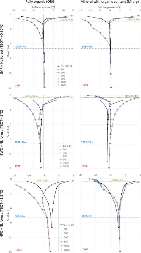
352                                                                 M. E. Elshamy et al.: Land surface modelling of permafrost

     – Active-layer thickness is defined as the maximum
       depth, measured from the ground surface, of the zero
       isotherm over the year taken from the annual maximum
       temperature envelopes by linear interpolation between
       layers bracketing the zero value (the freezing point de-
       pression is not considered) and has to be connected to
       the surface. The daily progression of ALT can also be
       generated to visualize the thaw and freeze fronts and
       determine the dates of thaw and freeze-up. These are
       calculated in a similar way to the annual ALT but using
       daily envelopes.
     – Depth of the zero annual amplitude (DZAA) is where
       the annual temperature envelopes meet within 0.1◦ (van
       Everdingen, 2005), and the temperature at this depth is
       TZAA.
Permafrost is usually defined as ground that remains cryotic
(i.e. temperature ≤ 0◦ C) for at least 2 years (Dobinski, 2011;
van Everdingen, 2005), but for modelling purposes and to
validate against annual ground temperature envelopes and              Figure 1. Schematic of the soil column showing the variables used
                                                                      to diagnose permafrost.
ALT observations, a 1-year cycle is adopted. This is common
amongst the climate and land surface modelling community
(e.g. Park et al., 2013). van Everdingen (2005) defined the           as the sum of the heat capacities, Cj , of its constituents (liq-
active-layer thickness as the thickness of the layer that is          uid water, ice, soil minerals, and organic matter), weighted
subject to annual thawing and freezing in areas underlain             by their volume fractions θj and, therefore, varies with time
by permafrost. Strictly speaking, the active-layer thickness          depending on the moisture content.
should be the lesser of the maximum seasonal frost depth                    X
and the maximum seasonal thaw depth (Walvoord and Kury-               Ci =      Cj θj                                               (2)
lyk, 2016). The maximum frost depth can be less than the                     j

maximum thaw depth, and, in such a case, there is a layer             Heat fluxes between soil layers are calculated using the layer
above the permafrost that is warmer than 0 ◦ C but is not con-        temperatures at each time step using the one-dimensional
nected to the surface (a lateral talik). Because active-layer         heat conduction equation
observations are usually based on measuring the maximum
                                                                                      dT
thaw depth, we adopted the same (thaw rather than freeze)             G (z) = −λ(z)      ,                                         (3)
criterion when calculating ALT in the model.                                          dz
   Prior versions of MESH/CLASS merely outputted tem-                 where λ(z) is the thermal conductivity of the soil calcu-
perature profiles. The code has been amended to calculate             lated analogously to the heat capacity. Temperature variation
the additional permafrost-related outputs detailed above. A           within each soil layer is assumed to follow a quadratic func-
typical CLASS configuration consists of 3 soil layers of 0.1,         tion of depth (z). Setting the flux at the bottom boundary to a
0.25, and 3.75 m thickness, but in 2006, the CLASS code               constant (i.e. Neumann-type boundary condition for the dif-
was amended to accommodate as many layers as needed                   ferential equation) and diagnosing the flux into the ground
(Verseghy, 2012). Neglecting lateral heat flow, the one-              surface, G(0), from the solution of the surface energy bal-
dimensional finite difference heat conservation equation is           ance results in a linear equation for G(0) as a function of T i
applied to each layer to obtain the change in average layer           for the different layers in addition to soil surface temperature,
temperature T i over a time step 1t as                                T (0). This enables the diagnosing of fluxes and temperatures
                             1t                                      of all layers using a forward explicit scheme. More details are
 t+1        t
        = T i + Gti−1 − Gti

Ti                                  ± Si ,                   (1)      given in Sect. S1 of the Supplement, and full details are given
                             Ci 1zi                                   in Verseghy (2012, 1991).
where t denotes the time, i is the layer index, Gi−1 and Gi              The CLASS thermal boundary condition at the bottom of
are the downward heat flux at the top and bottom of the soil          the soil column is either “no flux” (i.e. the gradient of the
layer, respectively, 1zi is the thickness of the layer, Ci is the     temperature profile should be zero) or a constant geother-
volumetric heat capacity, and Si is a correction term applied         mal flux. For this study, we considered the no-flux condi-
when the water phase changes (freezing or thawing) or the             tion, as data for the geothermal flux are not easy to find at
water percolates (exits the soil column at the lowest bound-          the Mackenzie River basin scale. Nicolsky et al. (2007) ig-
ary). The volumetric heat capacity of the layer is calculated         nored the geothermal flux in their study over Alaska using

Hydrol. Earth Syst. Sci., 24, 349–379, 2020                                          www.hydrol-earth-syst-sci.net/24/349/2020/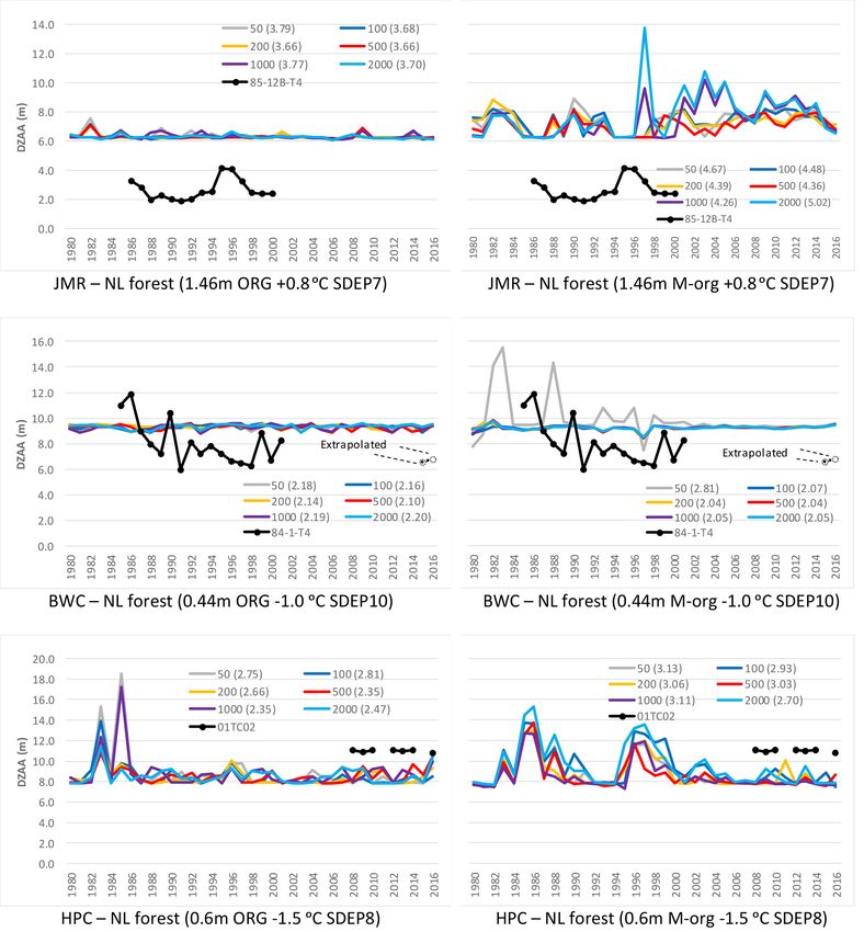
M. E. Elshamy et al.: Land surface modelling of permafrost                                                                     353

CLM with an 80 m soil column. Sapriza-Azuri et al. (2018)          thawing and its major impacts on landforms and connectiv-
showed that the difference in temperature at DZAA between          ity, and thus the hydrology of the basin. This is achieved
the two cases is within the error margin for geothermal tem-       through detailed studies conducted at three sites along a tran-
perature measurements for 60 % of their simulations at Nor-        sect near the Mackenzie River going from the sporadic per-
man Wells. However, we also tested with a constant geother-        mafrost zone (Jean Marie River) to the extensive discontinu-
mal flux to verify those previous findings.                        ous zone (Norman Wells) and the extensive continuous zone
   As for organic soils, CLASS can use a percentage of or-         (Havikpak Creek) as shown in Fig. 3. The following para-
ganic matter within a mineral soil layer, a fully organic layer,   graphs give brief descriptions of the three sites. Table 1 gives
or thermal and hydraulic properties provided directly. As the      details of permafrost monitoring at the sites, while more de-
latter are not usually available, especially at large scales, we   tailed descriptions are given in Sect. S2 of the Supplement.
used the first two options. In the first case, the organic con-       The Jean Marie River (JMR) is a tributary of the main
tent is used to modify soil hydraulic and thermal properties,      Mackenzie River basin (Fig. 3a) in the Northwest Territo-
similar to CLM (Oleson et al., 2013). For fully organic soils,     ries of Canada. The basin is dominated by boreal (deciduous,
CLASS has special values for those properties depending on         coniferous, and mixed) forest on raised peat plateaux and
the type of organic soil selected (fibric, hemic, or sapric)       bogs. The basin is located in the sporadic permafrost zone
based on the work of Letts et al. (2000) for peat soils (see       where permafrost underlies few spots only and is character-
Sect. S1). In traditional CLASS applications, when the flag        ized by warm temperatures (> −1 ◦ C) and limited (< 10 m)
for organic soil is activated, fibric (type 1) parameters are      thickness (Smith and Burgess, 2002). The basin and adja-
assigned to the first soil layer, hemic (type 2) parameters to     cent basins (e.g. Scotty Creek) have been subject to extensive
the second, and sapric (type 3) parameters to deeper layers        studies because the warm, thin, and sporadic permafrost un-
(Verseghy, 2012; see Supplement Table S1 for parameter val-        derling the region has been rapidly degrading (Calmels et al.,
ues). The corresponding code in MESH was amended such              2015; Quinton et al., 2011). Several permafrost monitoring
that more than one fibric or hemic layer can be present, and       sites have been established in and around the basin mostly
that the organic soil flag can be switched off (returning to       as part of the Norman Wells–Zama pipeline monitoring pro-
a mineral soil parameterization) for lower layers. In assign-      gram launched by the government of Canada and Enbridge
ing the organic-layer type, the same order is used (fibric at      Pipeline Inc. in 1984–1985 (Smith et al., 2004) to investigate
the surface, followed by hemic, then sapric with depth), as        the pipeline impact on permafrost conditions. This study uses
this represents the natural decomposition process. But with        data from sites 85-12A and 85-12B (see Table 1). Site 85-
the introduction of many more layers with depth, it is neces-      12A has no permafrost, while site 85-12B, in close proxim-
sary to have more flexibility in how the organic layers can be     ity, has a thin (3–4 m) permafrost layer with an ALT of about
configured. The fully organic parameterization was activated       1.5 m as estimated from soil temperature envelopes over the
when the organic content is 30 % or more, based on recom-          period 1986–2000. See Fig. S1 in the Supplement for a plot
mendation by the Soil Classification Working Group (1998).         of observed temperature envelopes.
                                                                      Bosworth Creek (BWC) has a small basin draining from
2.2   Study sites and permafrost data                              the northeast to the main Mackenzie River near Norman
                                                                   Wells (Fig. 3b). Permafrost monitoring activities started in
The Mackenzie River basin extends between 102–140◦ W               the region in 1984 with the construction of the Norman
and 52–69◦ N (Fig. 2). It drains an area of about 1.775 ×          Wells–Zama buried oil pipeline (as described above). The
106 km2 of western and northwestern Canada and covers              basin is dominated by boreal (deciduous, coniferous, and
parts of the provinces of Saskatchewan, Alberta, and British       mixed) forest. It is located in the extensive discontinuous per-
Colombia, as well as the Yukon and the Northwest Territo-          mafrost zone with relatively deep active-layer (1–3 m) and
ries (NWT). The average annual discharge at the basin out-         relatively thick (10–50 m) permafrost (Smith and Burgess,
let to the Beaufort Sea exceeds 300 km3 , which is the fifth       2002). Sapriza-Azuri et al. (2018) used cable T5 at the Pump
largest discharge to the Arctic. Such a large discharge influ-     Station 1 site (84-1) (see Table 1) to investigate the appropri-
ences regional as well as global circulation patterns under        ate soil depth and initial conditions for their permafrost sim-
the current climate, and it is expected to have implications       ulations, which serve as a pre-cursor for this current study.
for climate change. Figure 2 also shows the permafrost ex-         They recommended a soil depth of at least 20 m to ensure
tent and categories for the MRB taken from the Canadian            that the simulated DZAA is within the soil profile. However,
Permafrost Map (Hegginbottom et al., 1995). About 75 % of          they based their analysis on cable T5, which is within the
the basin is underlain by permafrost that can be either con-       right-of-way of the pipeline and is likely to be affected by
tinuous (in the far north and the western mountains), discon-      its construction or operation. We focus on the Norman Wells
tinuous (to the south of the continuous region), sporadic (in      Pump Station 1 site (84-1), and for this study we choose cable
the southern parts of the Liard and in the Hay sub-basin),         T4 as it is more likely to reflect the natural permafrost con-
or patchy further south. It is important to properly represent     ditions being out of the right of way of the pipeline. There
permafrost for the MRB model, given the current trends of

www.hydrol-earth-syst-sci.net/24/349/2020/                                         Hydrol. Earth Syst. Sci., 24, 349–379, 2020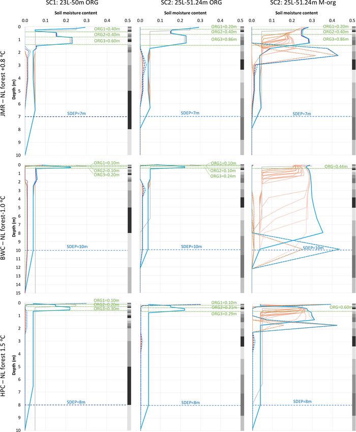
354                                                                    M. E. Elshamy et al.: Land surface modelling of permafrost

Table 1. Permafrost sites and important measurements for the study sites. NA: not available. KP: kilometre post (distance from the start of
the pipeline in Norman Wells). R.O.W.: right-of-way (of the pipeline).

  Site name                  Site ID            Type          Cables                 Record          Vegetation              Permafrost
                                                              (Depth in m)           period                                  condition
  JMR (Fort Simpson)
  Jean Marie Creek           JMC-01             Thermal       T1 (5)                 2008–2016       Shrub fen               No
                             JMC-02             Thermal       T1 (5)                 2008–2016       Needleleaf forest       No
  Pump Station 3             85-9 (NWZ9)        Thermal       T1 (5), T2 (5), T3     1986–1995,      Needleleaf forest/      No
                                                              (20), T4 (20)          2012–2016       shrubs/moss
  Jean Marie Creek A         85-12A             Thermal       T1 (5), T2 (5), T3     1986–1995                               No
                                                              (16.4), T4 (12)
  Jean Marie Creek B         85-12B             Thermal       T1 (5), T2 (5), T3     1986–2000                               Yes
                             (NWZ12)                          (17.2), T4 (9.7)
  Mackenzie Highway S        85-10A             Thermal       T1 (5), T2 (5), T3     1986–1995       NA                      No
                                                              (20), T4 (20)
                             85-10B             Thermal       T1 (5), T2 (5), T3     1986–1995       NA                      No
                                                              (10.5), T4 (10.5)
  Moraine South              85-11              Thermal       T1 (5), T2 (5), T3     1986–1995,      NA                      No
                                                              (12), T4 (12)          2014–2016
  BWC (Norman Wells)
  Norman Wells Fen           99-TT-05           Thaw tube                            2009            Needleleaf forest/      Yes
                             99-TC-05           Thermal       Near surface           2004–2008       moss
  Normal Wells Town          Arena              Thermal       T1 (16)                2014–2015       Disturbed area ad-      Yes
                             WTP                Thermal       T1 (30)                2014–2017       jacent to parking lot   Yes
  KP 2 – Off R.O.W.          94-TT-05           Thaw tube                            1995–2007       Needleleaf forest/      Yes
  Norman Wells (Pump         84-1               Thermal       T1 (5.1), T2 (5), T3   1985–2000       shrubs/moss             Yes
  Station 1)                                                  (10.4), T4 (13.6),     1985–2016
                                                              T5 (19.6)
  van Everdingen             30 m               Thermal       T1 (30)                2014–2017       Needleleaf/             Yes
                                                                                                     mixed forest
  Kee Scrap                  Kee Scrap-HT       Thermal       T1 (128)               2015–2017       Mixed forest            No
  HPC (Inuvik)
  Havikpak Creek             01-TT-02           Thaw tube                            1993–2017       Needleleaf forest       Yes
  Inuvik Airport             01-TT-03           Thaw tube                            2008–2017                               Yes
  Inuvik Airport             90-TT-16           Thaw tube                            2008                                    Yes
  Upper Air                  01-TT-02           Thaw tube                            2008–2017       NA                      Yes
  Inuvik Airport (Trees)     01-TC-02           Thermal       T1 (10)                2008–2017       Needleleaf forest       Yes
  Inuvik Airport (Bog)       01-TC-03           Thermal       T1 (8.35)                              Wetland                 Yes
                             12-TC-01           Thermal       T1 (6.5)               2013–2017                               Yes

Hydrol. Earth Syst. Sci., 24, 349–379, 2020                                             www.hydrol-earth-syst-sci.net/24/349/2020/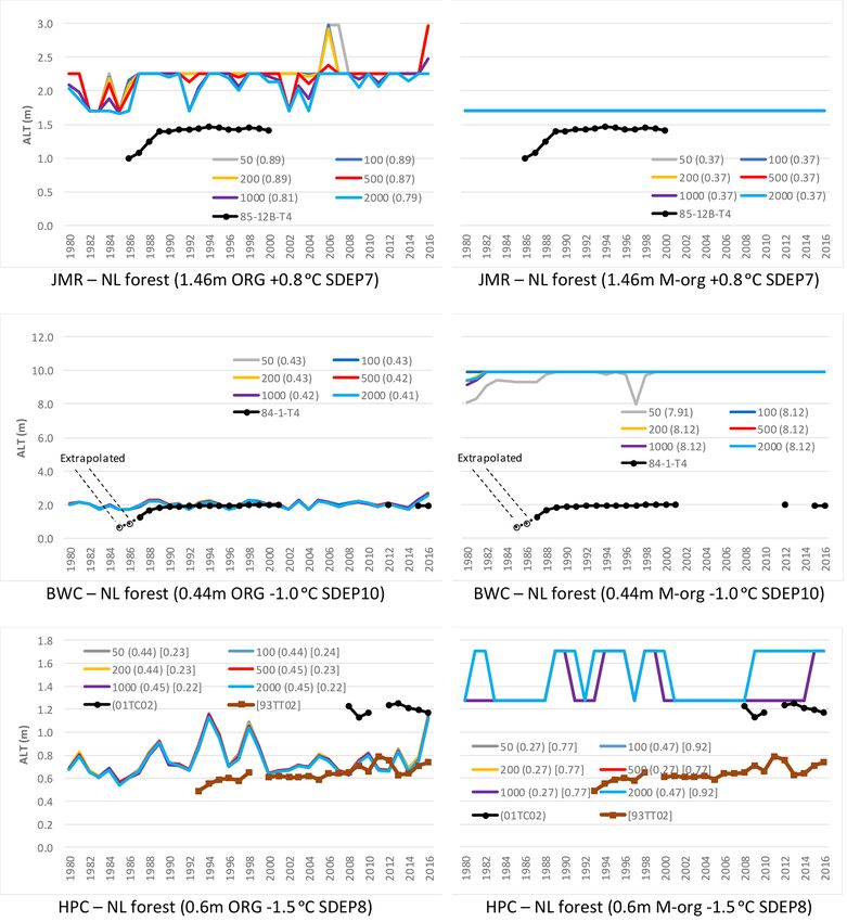
M. E. Elshamy et al.: Land surface modelling of permafrost                                                                           355

Figure 2. Mackenzie River basin: location, permafrost classification, and the three study sites.

has been a continuous record since 1985 (Smith et al., 2004;              (CCRS) 2005 dataset (Canada Centre for Remote Sensing et
Caroline Duchesne, personal communication, 2017).                         al., 2010). The parameterization of certain land cover types
   Havikpak Creek (HPC) is a small Arctic research basin                  differentiates between the eastern and western sides of the
(Fig. 3c) located in the eastern part of the Mackenzie River              basin using the Mackenzie River as a divide, informed by
basin delta, 2 km north of Inuvik Airport in the Northwest                calibrations of the MRB model. HPC and BWC are on the
Territories. The basin is dominated by sparse taiga forest                east side of the river, while JMR is on the west side, and
and shrubs and is underlain by thick permafrost (> 300 m).                therefore these setups have different parameter values for cer-
The basin has been subject to several hydrological studies,               tain GRU types (e.g. needleleaf forest). SDEP, soil texture
especially during the Mackenzie GEWEX (Global Energy                      information, and initial conditions were taken as described
and Water Exchanges) Study (MAGS). Recently, Krogh et                     above and adjusted according to model evaluation versus
al. (2017) modelled its hydrological and permafrost condi-                permafrost-related observations (ALT, DZAA, and temper-
tions using the Cold Regional Hydrological Model (CRHM)                   ature envelopes) with the aim of developing an initialization
(Pomeroy et al., 2007). They integrated a ground freeze and               and configuration strategy that can be implemented for the
thaw algorithm called XG (Changwei and Gough, 2013)                       larger MRB model.
within CRHM to simulate the active-layer thickness and the                   Provisions for special land covers within the MESH
progression of the freeze and thaw front with time, but they              framework include inland water. Because of limitations in the
did not attempt to simulate the temperature envelopes or                  current model framework, inland water must be represented
DZAA. Ground temperatures are measured with tempera-                      as a porous soil. This is parameterized such that it remains
ture cables installed in boreholes at two sites, 01TC02 and               as saturated as possible, drainage is prohibited from the bot-
01TC03, respectively (Smith et al., 2016). In addition, there             tom of the soil column, and it is modelled using CLASS with
are three thaw tubes at the Inuvik Upper Air station (90-TT-              a large hydraulic conductivity value and no slope. Addition-
16) just to the west of the basin, at HPC proper (93-TT-02),              ally, it was initialized to have a positive bottom temperature,
and at the Inuvik Airport (Bog) site (01-TT-03) measuring                 and therefore, it does not develop permafrost. Wetlands are
the active-layer depth and ground settlement (Smith et al.,               treated in a similar way (impeded drainage and no slope) but
2009).                                                                    with grassy vegetation and preserving the soil parameteriza-
                                                                          tion as described in below in Sect. 2.5 and 2.6. It remains
2.3   Land cover parameterization                                         close to saturation but can still be underlain by permafrost,
                                                                          depending on location. Taliks are allowed to develop under
                                                                          wetlands this way.
Parameterizations for the three selected basins were ex-
tracted from a larger MRB model, described in Elshamy
et al. (2020). This includes the land cover characterization
and parameters for vegetation and hydrology. The land cover
data are based on the Canada Centre for Remote Sensing

www.hydrol-earth-syst-sci.net/24/349/2020/                                                 Hydrol. Earth Syst. Sci., 24, 349–379, 2020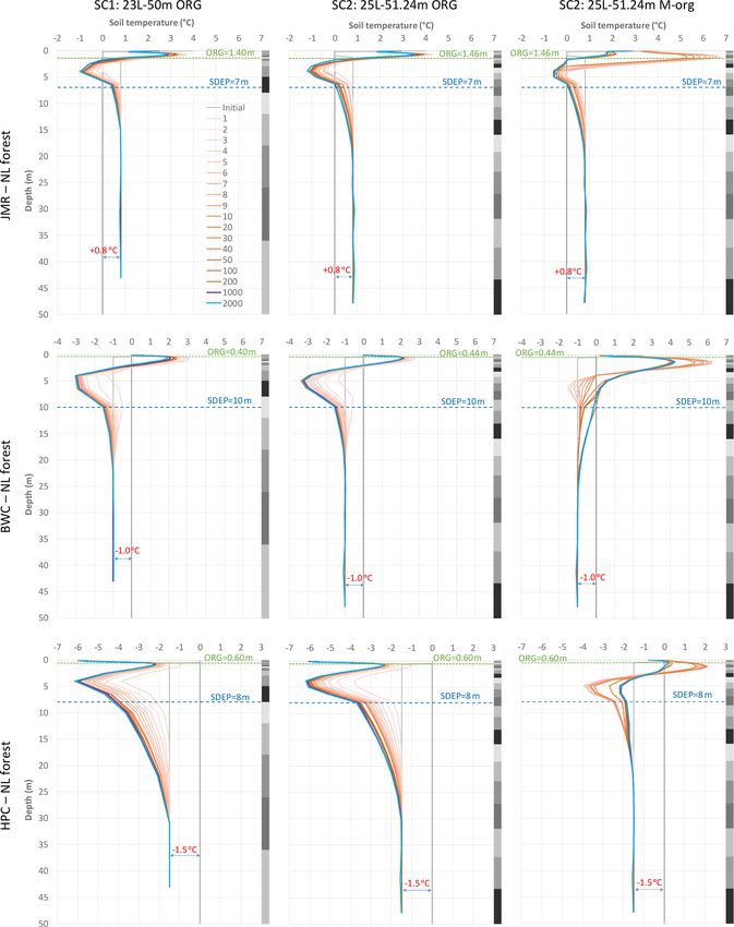
356                                                           M. E. Elshamy et al.: Land surface modelling of permafrost

Figure 3. Location of and permafrost measurement sites in the (a) Jean Marie River sub-basin, (b) Bosworth Creek sub-basin, and
(c) Havikpak Creek sub-basin.

Hydrol. Earth Syst. Sci., 24, 349–379, 2020                                     www.hydrol-earth-syst-sci.net/24/349/2020/
M. E. Elshamy et al.: Land surface modelling of permafrost                                                                       357

2.4   Climate forcing                                                depth is adequate at the three sites selected in the subsequent
                                                                     sections.
MESH requires seven climatic variables at a sub-daily time              As noted above, the total soil column depth is only one
step to drive CLASS. For this study we used the WFDEI                factor in the configuration of the soil. The layering is as
(WATer and global CHange (WATCH) Forcing Data (WFD)                  critical. In former modelling studies, exponentially increas-
with the ERA-Interim analysis from the European Centre               ing soil layer thicknesses were used, aiming to reach the
for Medium-Range Weather Forecasts) dataset that covers              required depth with a minimum number of layers. The ex-
the period 1979–2016 at 3-hourly resolution (Weedon et al.,          ponential formulation creates more layers near the surface,
2014). The dataset was linearly interpolated from its original       which allows the models to capture the strong soil moisture
0.5◦ × 0.5◦ resolution to the MRB model grid resolution of           and temperature gradients there and yet have a reasonable
0.125◦ × 0.125◦ . The high resolution forecasts of the Global        number of layers (15–20) to reduce the computational bur-
Environmental Multiscale (GEM) atmospheric model (Côté               den. However, for most of the MRB, the observed ALT is
et al., 1998b, a; Yeh et al., 2002) and the Canadian Precipi-        in the range of 1–2 m from the surface, and the exponential
tation Analysis (CaPA; Mahfouf et al., 2007) datasets, often         formulations increase layer thickness quickly after the first
combined as GEM-CaPA, provide the most accurate gridded              0.5–1.0 m, which reduces the accuracy of the model, espe-
climatic dataset for Canada in general (Wong et al., 2017).          cially for transient simulations. Therefore, we adopted two
Unfortunately, these datasets are not available prior to 2002        layering schemes that have more layers in the top 2 m and
when most of the permafrost observations used for model              increased layer thicknesses at lower depths to a total depth
evaluation are available. However, an analysis by Wong et            near 50 m. The first scheme has the first metre divided into
al. (2017) showed that precipitation estimates from the CaPA         10 layers, the second metre divided into 5 layers, and the to-
and WFDEI products are in reasonable agreement with sta-             tal soil column has 23 layers. The second scheme has soil
tion observations. Alternative datasets such as WFD (Wee-            thicknesses increasing more gradually to reach 51.24 m in 25
don et al., 2011) and Princeton (Sheffield et al., 2006) go          layers following a scaled power law. This latter scheme has
earlier in time (1901) but are not being updated (WFD stops          the advantage that each layer is always thicker than the one
in 2001, while Princeton stops in 2012). Additionally, Wong          above it (except the second layer), as the explicit forward
et al. (2017) showed that the Princeton dataset has large pre-       difference numerical scheme to solve the energy and water
cipitation biases for many parts of Canada. Analysis of the          balances in CLASS can have instabilities when layers in suc-
sensitivity of the results presented here regarding the choice       cession have the same thickness. The minimum soil layer
of the climatic dataset is beyond the scope of this work.            thickness is taken as 10 cm as advised by Verseghy (2012).
                                                                     Table 2 shows the soil layer thicknesses and centers (used
2.5   Soil profile and permeable depth                               for plotting temperature profiles and envelopes) for both soil
                                                                     layering schemes.
As mentioned earlier, Sapriza-Azuri et al. (2018) recom-                As mentioned before, the permeable depth marks the hy-
mended a total soil column depth (D) of no less than 20 m            drologically active horizon below which the soil is not per-
to enable reliable simulation of permafrost dynamics con-            meable and where its thermal properties are changed to those
sidering the uncertainties involved mainly due to parame-            of bedrock material. This makes it an important parameter for
ters. Their study is relevant because they used the same             not only for water storage but also for thermal conductance.
model used in this study (MESH/CLASS). They studied sev-             It was set for the various study basins from the Shangguan et
eral profiles, down to 71.6 m depth. Recent applications of          al. (2017) dataset interpolated to 0.125◦ and the MRB model
other H-LSMs also considered deep soil column depths; e.g.           grid resolution by Keshav et al. (2019b). The sensitivity of
CLM 4.5 used 42.1 m (Oleson et al., 2013), and CHANGE                the results to SDEP is assessed by perturbing it within a rea-
(Park et al., 2013) used 30.5 m. After a few test trials with        sonable range at each site as shown in the results.
D = 20, 25, 30, 40, 50 and 100 m at the study sites, we found
that the additional computation time when adding more lay-           2.6   Configuration of organic soil
ers to increase D is outweighed by the reliability of the simu-
lations. The reliability criterion used here is that the tempera-    Organic soils were mapped from the Soil Landscapes of
ture envelopes meet (i.e. DZAA) well within the soil column          Canada (SLC) v2.2 dataset (Centre for Land and Biologi-
depth over the simulation period (including spin-up) such            cal Resources Research, 1996) for the whole MRB (Fig. 4)
that the bottom boundary condition does not disturb the sim-         at 0.125◦ resolution by Keshav et al. (2019a). However, this
ulated temperature profiles and envelopes and ALT (Nicolsky          dataset does not provide information on the depth of the or-
et al., 2007). DZAA is a relatively stable indicator for this cri-   ganic layers or their configuration (i.e. the thicknesses of fib-
terion (Alexeev et al., 2007). The simulated DZAA reached a          ric, hemic, and sapric layers in peaty soils). Therefore, differ-
maximum of 20 m at one of the sites in a few years, and thus         ent configurations have been tested at the study sites based on
a total depth of 50 m was used in anticipation for possible          available local information (Table 3). We also compared fully
changes in DZAA with future warming. We show that this               organic configurations (ORG) at the three sites with mineral

www.hydrol-earth-syst-sci.net/24/349/2020/                                           Hydrol. Earth Syst. Sci., 24, 349–379, 2020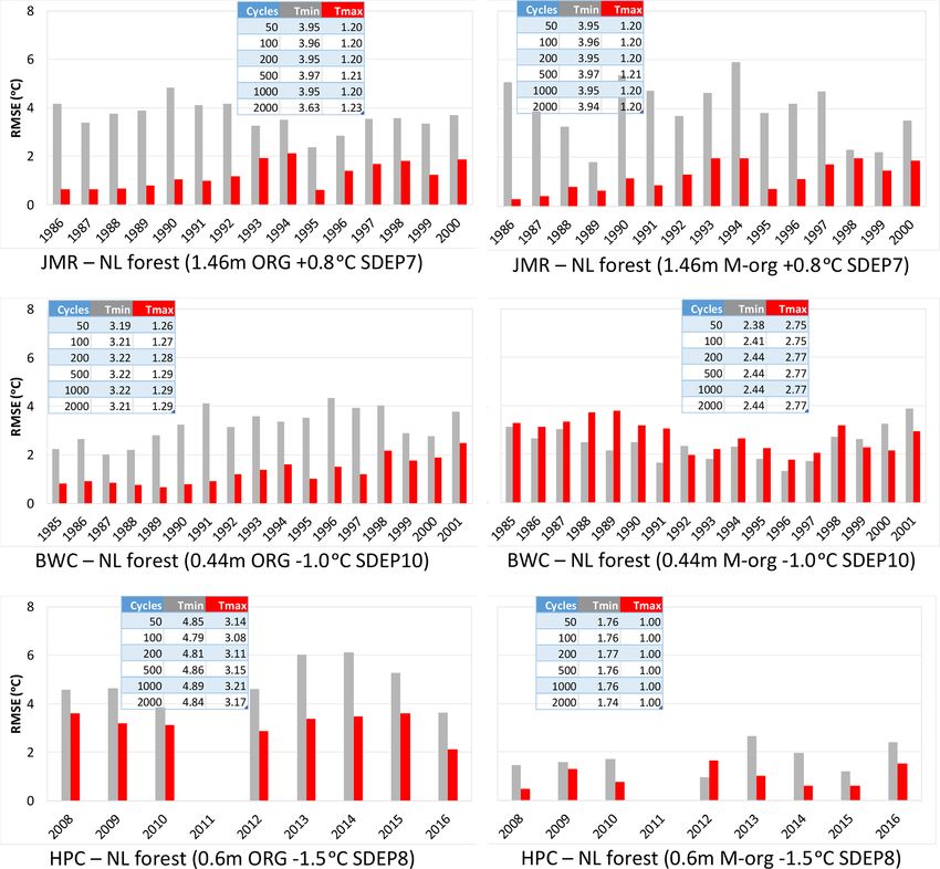
358 M. E. Elshamy et al.: Land surface modelling of permafrost
configurations with organic content (M-org) to investigate assessed visually using various plots as well as by comput-
the appropriate configuration at each site, keeping in mind ing the difference between each cycle and the previous one
the need to generalize it for larger basins. making sure the absolute difference does not exceed 0.1 ◦ C
For JMR, we tested configurations with about 0.3 m or- for temperature (which is the accuracy of measurement of the
ganic soil (three layers) to over 2 m of organic soil, where temperature sensors) and 0.01 m3 m−3 for moisture compo-
organic content from SLC v2.2 ranged between 48 %–59 % nents for all soil layers. The aim is to determine the minimum
(Fig. 4). The soil texture immediately below these layers was number of cycles that could inform the ongoing development
characterized as a mineral soil of uniform texture with 15 % of the MRB model, as it is computationally very expensive to
sand and 15 % clay content, with the remainder assigned as spin up the whole MRB domain for 2000 cycles. We then as-
silt. Peat depths of 4–7 m in the surrounding region have sessed the impact of running the model for the period 1980–
been identified in reports (Quinton et al., 2011) and by bore- 2016 after 50, 100, 200, 500, 1000, and 2000 spin-up cycles
hole data at permafrost monitoring sites (Smith et al., 2004). on ALT, DZAA, and the temperature envelopes at the three
Therefore, layers at these depths until bedrock were char- sites for selected years depending on the available observa-
acterized as mineral soils (as described above), but they had tions. We assessed the quality of the simulations visually as
50 % organic content. These deeper layers, while having con- well as quantitatively by calculating the root mean squared
siderable organic content, do not use the previously described error (RMSE) for ALT, DZAA, and the temperature profiles.
parameterization for fully organic soils. This is an exception
for this basin, which could be generalized for the MRB in ar-
eas with high organic content (e.g. > 50 %) like this region. 3 Results
These configurations are summarized in Table 3. For the M-
3.1 Establishing initial conditions
org configuration, we used a decreasing organic content with
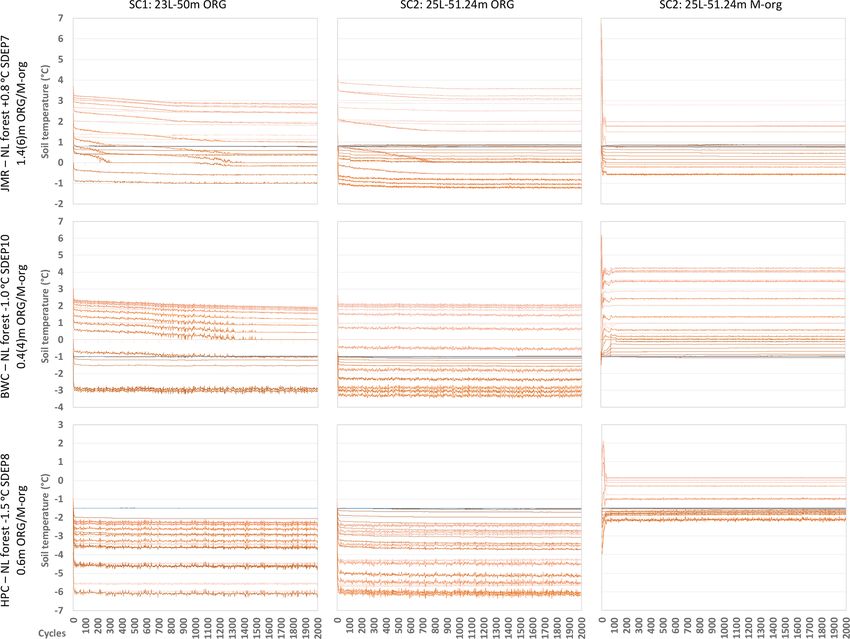
depth. Figure 5 shows the temperature profiles at the end of spin-
For BWC, the organic map indicated that organic matter ning cycles for a selected GRU (needleleaf forest; NL) for
ranges between 27 %–34 %. We tested configurations with the three selected sites using the two suggested soil layer-
0.3–0.8 m organic layers. A borehole log for the 84-1-T4 site ing schemes (SC1 and SC2) and using two different organic
(Smith et al., 2004) shows a thin organic silty layer at the top configuration (ORG and M-org) for SC2. NL forest is repre-
(close to 0.2–0.3 m). Sand and clay content below the organic sentative of the vegetation at the selected thermal sites for the
layers are uniformly taken to be 24 % and 24 % respectively three studied basins (except the HPC bog site). As expected,
based again on SLC v2.2, with the remainder (52 %) assumed the profile changes quickly for the first few cycles then tends
to be silt. We tested ORG and M-org configurations as shown to stabilize such that no significant change occurs after 100
in Table 3. cycles and less in most cases. Similar observations can be
The organic content indicated by the gridded soil infor- made for soil moisture (both water and ice contents) from
mation at HPC is only 18 %, which is lower than the 30 % Fig. 6. Changes in moisture content tend to diminish more
threshold decided for fully organic soils. However, Quin- quickly than those for temperature, especially for ORG, and
ton and Marsh (1999) used a 0.5 m thick organic layer in thus we will focus on temperature changes in the remaining
their conceptual framework developed to characterize runoff results. However, water and ice fractions play important roles
generation in the nearby Siksik Creek. Krogh et al. (2017) in defining the thermal properties of the soil and provide use-
adopted the same depth for their modelling study of HPC. ful insights to understand certain behaviours in the simula-
Therefore, we tested configurations with 0.3–0.8 m fully or- tions. Figure 7 shows the temperature of each layer for the
ganic layers as well as the M-org configuration with a uni- same cases versus the cycle number to visualize the patterns
form 18 % organic content. Below that, soil texture values of change over the cycles. Small oscillations are observed, in-
are taken to be 24 % sand and 32 % clay from SLC v2.2. dicating minor numerical instabilities in the model, but these
do not cause major differences for the simulations. In some
2.7 Spin-up and stabilization cases, the temperature keeps drifting for several hundred cy-
cles before stabilizing (if stabilization occurs). We note a few
We used the first hydrological year of the climate forcing important findings:
(October 1979–September 1980) to spin up the model re-
peatedly for 2000 cycles while monitoring the temperature – The temperature of the bottom layer (TBOT) remains
and moisture (water and ice contents) profiles at the end of virtually unchanged from its initial value. This triggered
each cycle for stabilization. We checked that the selected year further testing using different initial values, and the im-
was close to average in terms of temperature and precipita- pacts on stabilization were similar, as shown in the next
tion compared to the WFDEI record (1979–2016) as shown sections. We also checked the model behaviour for shal-
in Table 4. The start of the hydrological year was selected lower soil columns and found that the bottom tempera-
because it is easier to initialize CLASS when there is no ture did change during spin-up, within a range that de-
snow cover or frozen soil moisture content. Stabilization is creased as the total soil depth increased.
Hydrol. Earth Syst. Sci., 24, 349–379, 2020 www.hydrol-earth-syst-sci.net/24/349/2020/M. E. Elshamy et al.: Land surface modelling of permafrost 359
Table 2. Soil profile layering schemes.
First scheme (SC1) Second scheme (SC2)
Layer Thickness Bottom Center Thickness Bottom Center
1 0.10 0.10 0.05 0.10 0.10 0.05
2 0.10 0.20 0.15 0.10 0.20 0.15
3 0.10 0.30 0.25 0.11 0.31 0.26
4 0.10 0.40 0.35 0.13 0.44 0.38
5 0.10 0.50 0.45 0.16 0.60 0.52
6 0.10 0.60 0.55 0.21 0.81 0.71
7 0.10 0.70 0.65 0.28 1.09 0.95
8 0.10 0.80 0.75 0.37 1.46 1.28
9 0.10 0.90 0.85 0.48 1.94 1.70
10 0.10 1.00 0.95 0.63 2.57 2.26
11 0.20 1.20 1.10 0.80 3.37 2.97
12 0.20 1.40 1.30 0.99 4.36 3.87
13 0.20 1.60 1.50 1.22 5.58 4.97
14 0.20 1.80 1.70 1.48 7.06 6.32
15 0.20 2.00 1.90 1.78 8.84 7.95
16 1.00 3.00 2.50 2.11 10.95 9.90
17 2.00 5.00 4.00 2.48 13.43 12.19
18 3.00 8.00 6.50 2.88 16.31 14.87
19 4.00 12.00 10.00 3.33 19.64 17.98
20 6.00 18.00 15.00 3.81 23.45 21.55
21 8.00 26.00 22.00 4.34 27.79 25.62
22 10.00 36.00 31.00 4.90 32.69 30.24
23 14.00 50.00 43.00 5.51 38.20 35.45
24 6.17 44.37 41.29
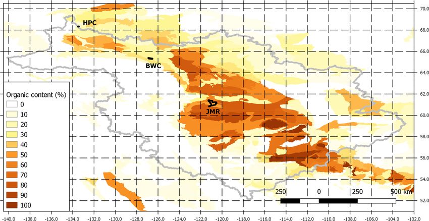
25 6.87 51.24 47.81
Figure 4. Gridded organic matter in soil at 0.125◦ resolution for the MRB, processed from the Soil Landscapes of Canada (SLC) v2.2 dataset
(Centre for Land and Biological Resources Research, 1996).
www.hydrol-earth-syst-sci.net/24/349/2020/ Hydrol. Earth Syst. Sci., 24, 349–379, 2020360 M. E. Elshamy et al.: Land surface modelling of permafrost
Table 3. The number of layers of each organic sub-type for fully organic soil configurations (ORG) and organic content for mineral configu-
rations (M-org).
Number of organic Organic sub-type (ORG) Organic content percentage (M-org)
layers 1 (Fibric) 2 (Hemic) 3 (Sapric) JMR BWC HPC
3 1 1 1 3@18, 0 →
4 1 1 2 2@35, 30, 4@18, 0 →
25, 0 →
5 1 2 2 4@18, 0 →
6 2 2 2 4@18, 0 →
8∗ 2 3 3 2@60, 2@50,
2@40, 30 →
10∗ 3 3 4
11∗ 3 4 4
∗ Only used for JMR; x @y means x layers with the specified percentage, and x → means the value is for the remainder of the layers below.
Table 4. Comparison of temperature and precipitation of the selected spinning year to mean climate of the WFDEI Dataset.
Site Mean annual temperature (◦ C) Total annual precipitation
(mm yr−1 )
WFDEI 1979–2016 Oct 1979– WFDEI 1979–2016 Oct 1979–
Mean SD Sep 1980 Mean SD Sep 1980
JMR −2.65 1.06 −1.81 418.1 64.5 338.4
BWC −5.65 1.01 −4.36 403.9 74.7 394.3
HPC −8.73 1.17 −7.82 295.7 40.0 301.2
– The vertical discretization of the soil plays an important content at some depth, which depends on the thickness of the
role in the evolution of temporal moisture and tempera- organic layers and the general site conditions. For example, it
ture profiles. SC2 results in faster stabilization than SC1 forms below the thick organic layers for JMR, but it formed
with less drifting for all cases. at a deeper depth at BWC as the organic thickness is smaller.
HPC has a comparable organic depth to BWC, but the layers
– The depth of organic layers, and their sub-type in fully
with high ice content formed at a shallower depth because the
organic soils, controls the shape of the moisture con-
site is colder. At all three sites, and for both ORG and M-org
tent profiles and the ice and water content partition-
configurations, there is a change in the slope of the temper-
ing. This in turn influences the soil thermal properties
ature profile at the depth corresponding to the interface of
(drier soils are generally less conductive, and icy soils
the soil to bedrock, illustrating the importance of the SDEP
are more conductive) and thus affects the number of cy-
parameter for permafrost simulations. This is caused by the
cles needed to reach stable conditions. Deeper fully or-
change in soil thermal properties above and below SDEP (re-
ganic soils (JMR) require more cycles to stabilize than
spective of the two different mediums above and below this
mineral ones with organic content.
interface) and the moisture contents therein; bedrock is as-
The temperature gradient northward is clear comparing the sumed to remain dry at all times, while soil will always have
different sites as well as the impact of the deeper organic lay- a minimum liquid water content depending on its type.
ers at JMR on the slower stabilization of temperature and, to Given the above findings, the remainder of the results
a lesser extent, moisture content. This is related to the low focus on SC2 only. Additionally, we considered different
thermal conductivity of organic matter as well as the low values for the bottom temperature based on site location
moisture content below the organic layers as peat acts as a and the extrapolation of observed temperature profiles. This
sponge absorbing water and heat and disallowing downward is because it cannot be established through spin-up, and
propagation, especially in the absence of ice (i.e. in summer). ground temperature measurements rarely go deeper than
Hemic and sapric peat soils have relatively high minimum 20 m. There are established strong correlations between near-
water contents as shown in Fig. 6 (see also Table S1 in the surface ground temperature and air temperature at the annual
Supplement). The M-org configuration allows more moisture scale (e.g. Smith and Burgess, 2000), but the near-surface
to seep below the organic layers and have some higher ice ground temperature is taken just a few centimetres below the
Hydrol. Earth Syst. Sci., 24, 349–379, 2020 www.hydrol-earth-syst-sci.net/24/349/2020/M. E. Elshamy et al.: Land surface modelling of permafrost 361 Figure 5. Soil temperature profiles at the end of selected spin-up cycles for the NL forest GRU at all three sites using different soil layering schemes and organic configurations; grey bars on the side indicate soil layers. surface. We spin up the model at the three sites for 2000 cy- results to SDEP, TBOT, and the organic soil depth will then cles for a few cases and then use the initial conditions after a be assessed using 100 spin cycles only. selected number of cycles to run a simulation for the period of record (1979–2016) and assess the differences for ALT, DZAA, and the temperature profiles. The sensitivity of the www.hydrol-earth-syst-sci.net/24/349/2020/ Hydrol. Earth Syst. Sci., 24, 349–379, 2020
362                                                                   M. E. Elshamy et al.: Land surface modelling of permafrost

Figure 6. Soil moisture profiles at the end of selected spin-up cycles for the NL forest GRU at all three sites using different soil layering
schemes and organic configurations. Solid lines indicate liquid, and dashed lines indicate ice. Grey bars on the side indicate soil layers. The
legend is as in Fig. 5.

3.2   Impact of spin-up                                                   figuration for SDEP, TBOT, and ORG and M-org. Most dif-
                                                                          ferences across the spin-up range are negligible. What stands
Figures 8, 9, and 10 show the simulated ALT, DZAA and                     out are some large differences in ALT and DZAA at JMR for
temperature envelopes (selected years) at the three study sites           some years (ORG configuration only) depending on the ini-
respectively using initial conditions after 50, 100, 200, 500,            tial conditions (i.e. number of cycles) used. The low thermal
1000, and 2000 spin-up cycles using SC2 and the stated con-               conductivity of the thick fully organic layers slows the stabi-

Hydrol. Earth Syst. Sci., 24, 349–379, 2020                                               www.hydrol-earth-syst-sci.net/24/349/2020/
M. E. Elshamy et al.: Land surface modelling of permafrost 363 Figure 7. Impact of the soil layering scheme selection on spin-up convergence at the three study sites (the darker the colour, the deeper the layer; the deepest layer is coloured blue). lization process and thus yields slightly different initial con- figuration. The M-org configuration does better for a mean ditions depending on the number of cycles used. That does ALT at JMR but is much worse than ORG for BWC which not happen for the two other sites with thinner ORG layers overestimates ALT by about 8 m. For BWC, the ALT simu- or for M-org configurations. This is further emphasized by lation under ORG is close to observations for most years, but the RMSE values for ALT and DZAA shown in the legends the simulation shows more interannual variability, while ob- of Figs. 8 and 9. servations show a small upward trend after an initial period Assuming that more spin-up cycles would lead to dimin- of a large increase (1988–1992), which may be the result of ished differences, and thus considering the results initiated the disturbance of establishing the site. A couple of obser- after 2000 cycles as a benchmark, one can accept an error of vations are marked “extrapolated” as the zero isotherm falls a few centimetres in the simulated ALT using a smaller num- above the first thermistor (located 1 m deep). For HPC, M- ber of spin-up cycles. For JMR, this error is about 10 % on org better represents the conditions at 01-TC-02, while ORG, average, which is much smaller than the error in simulating resulting in a smaller ALT on average, is closer to the thaw ALT at this site. Thus, there is a trade-off in computational tube measurements at HPC (93-TT-02), as indicated by the time by limiting the number of cycles required for a slight RMSE values. This is indicative of the large heterogeneity of loss of accuracy at some sites, particularly those located in conditions that can occur in close proximity to each other and the more challenging sporadic zone. that require different modelling configurations. M-org con- The figures also include relevant observations and RMSE figurations generally show little to no interannual variability values to assess the quality of simulations. The simulated (except for HPC), while ORG ones show more interannual ALT at JMR are overestimated (Fig. 8) by the ORG con- variability. www.hydrol-earth-syst-sci.net/24/349/2020/ Hydrol. Earth Syst. Sci., 24, 349–379, 2020
364                                                                  M. E. Elshamy et al.: Land surface modelling of permafrost

Figure 8. Impact of the number of spin-up cycles on the simulated ALT for the needleleaf forest GRU at all sites. Two organic configurations
were used for each site using the SC2 layering scheme; RMSE is shown in parenthesis.

   The simulated DZAA (Fig. 9) is overestimated at JMR un-              for HPC, which is less than half the total soil depth. This in-
der both ORG and M-org configurations, while it is close                dicates that a smaller soil column depth would not be suitable
to values deduced from observations at BWC and HPC. In                  for HPC but could be used for JMR and BWC.
contrast to ALT, DZAA observations have larger interannual                 Comparing temperature profiles for a selected year at each
variability than simulations, possibly due to the large spac-           site (Fig. 10) reveals a large difference between ORG and M-
ing of measuring thermistors and the failure of some in some            org configurations, especially at HPC and BWC. The over-
years. For HPC, both ORG and M-org simulations are show-                all shapes of the profiles depend on the selected configura-
ing more variability in DZAA than the depth deduced from                tion. M-org works better for HPC, while ORG is better at
observations for 01-TC-02, and both underestimate it. In gen-           BWC. Both configurations do relatively well for JMR, al-
eral, matching DZAA to observations is not an objective in              though this site is characterized with deep peat. At BWC,
itself, but its occurrence well within the selected soil depth          the ORG simulation agrees well with observations in terms
is more important. The largest value simulated is about 19 m            of ALT, but the temperature envelopes are generally colder

Hydrol. Earth Syst. Sci., 24, 349–379, 2020                                              www.hydrol-earth-syst-sci.net/24/349/2020/
You can also read