TVA in the wild: Applying the theory of visual attention to game-like and less controlled experiments
←
→
Page content transcription
If your browser does not render page correctly, please read the page content below
Open Psychology 2021; 3:1–46

Research Article

Alexander Krüger*, Jan Tünnermann*, Lukas Stratmann, Lucas Briese, Falko Dressler,
and Ingrid Scharlau

TVA in the wild: Applying the theory of visual
attention to game-like and less controlled
experiments
https://doi.org/10.1515/psych-2021-0001
Received Jan 31, 2020; accepted Nov 09, 2020

Abstract: As a formal theory, Bundesen’s theory of visual attention (TVA) enables the estimation of several
theoretically meaningful parameters involved in attentional selection and visual encoding. As of yet, TVA has
almost exclusively been used in restricted empirical scenarios such as whole and partial report and with strictly
controlled stimulus material. We present a series of experiments in which we test whether the advantages
of TVA can be exploited in more realistic scenarios with varying degree of stimulus control. This includes
brief experimental sessions conducted on different mobile devices, computer games, and a driving simulator.
Overall, six experiments demonstrate that the TVA parameters for processing capacity and attentional weight
can be measured with sufficient precision in less controlled scenarios and that the results do not deviate
strongly from typical laboratory results, although some systematic differences were found.

Keywords: theory of visual attention; TVA; modeling; capacity; attentional weight; gamification; salience;
Bayesian parameter estimation

1 Introduction
In most areas, psychological research methods stress the value of strict control: According to common psy-
chological thinking, drawing conclusions from data presupposes an appropriate choice and manipulation
of independent variables, tight control of possible confounding factors, reduction of random noise, and
randomization of participants. In more everyday settings—“in the wild”—such control would not be possible
which is one of the main reasons to study phenomena in the laboratory.
     However, through the reproducibility crisis (e.g., Open Science Collaboration, 2015), we have learned that
even data obtained in controlled laboratory studies are far less reliable than had been expected. We do not
aim to get into details of what can be expected in terms of reproducibility and what the causes of the present
crisis are (for a summary of potential problems with scientific practices in psychology see, e.g, Chambers,
2017), but want to stress one of those causes, a lack of cumulative theory (Muthukrishna and Henrich, 2004).
Without theoretical frameworks and respective formal models, it is difficult to come up with precise and
unambiguous predictions for yet unobserved situations that allow testing hypotheses. If these predictions are
not precise and do not adhere to some formal framework, separating expected from unexpected results is
difficult and undesired flexibility when interpreting results can hinder true progress. Theoretical frameworks

*Corresponding Author: Alexander Krüger: Paderborn University, Faculty of Arts and Humanities, Psychology
*Corresponding Author: Jan Tünnermann: University of Marburg, Department of Psychology
Alexander Krüger and Jan Tünnermann share first authorship
Lukas Stratmann, Falko Dressler: TU Berlin, School of Electrical Engineering and Computer Science
Lucas Briese: Paderborn University, Faculty of Electrical Engineering, Computer Science and Mathematics
Ingrid Scharlau: Paderborn University, Faculty of Arts and Humanities, Psychology

  Open Access. © 2021 A. Krüger et al., published by De Gruyter.         This work is licensed under the Creative Commons
Attribution 4.0 License
2 | A. Krüger et al.

also enable the consistent use of more than one empirical approach per research question and provide a
means for integration across different disciplines.
     In the present article, we explore a new approach in the field of visual processing and selective attention
in which we turn around the usual scheme: Instead of adhering to the strictest laboratory settings and model-
free null-hypothesis significance testing, we employ more flexible game-like experimental paradigms with
rigorous models that formally link the results of the different experiments we conduct and existing findings
in the literature. Our question is to which degree results obtained under such conditions match up with
measurements obtained with a lab- and model-based agenda. Nested in this overall question, we also ask
whether orientation and color salience bias temporal-order judgments as reported in earlier studies (Krüger
et al., 2016, 2017).
     Administering fundamental attention experiments in a more flexible, game-like manner potentially brings
many advantages that might make up for the loss in experimental control and a possibly increased (but
quantifiable) uncertainty in the results. For instance, more flexible experiments could be delivered via app
stores and web browsers to large and diverse participant pools and motivational elements can be more easily
integrated in game-like scenarios. In the end, easy large-scale access, flow and motivation, combined with a
model-based evaluation could lead to a superior overall data quality despite losses in experimental control.

1.1 A simple task and model for investigating visual processing and selective
    attention “in the wild”

Formal models are an important means to foster cumulative theory and an important part of scientific progress.
Many topics have a research history of several decades, and it is almost indefensible not to try to formalize
the core knowledge that researchers have already obtained. Verbal research summaries are poor surrogates
for this (Meehl, 1990); they may help to derive hypotheses that can be put to an empirical test, but are prone
to inexactness and ambiguity and much less suited for describing complex relationships between possible
influences.
     Put very generally, the main function of a formal model in empirical sciences is to connect theoretical
considerations and data. Models are customizations of theories such that these become applicable to some of
the concrete properties of the phenomena by filling in the gaps between latent causes and data (Bailer-Jones,
2009). According to Bailer-Jones, two important parts of modeling are the theoretical model and the data
model. The theoretical model is derived from the theory, and it is necessary as a model of the situation in
which the data is observed. It represents the theoretical considerations in a specific situation. The data model
is necessary to deal with the uncertainty arising from data collection in a specific experiment, for instance
measurement uncertainty. Modeling thus provides a tight coupling of theory and data (Krüger et al., 2018).
     For the present work, we derive a formal model from Bundesen’s theory of visual attention (TVA; Bundesen,
1990; Bundesen and Habekost, 2008). Its parameters are defined theoretically and cognitively specific (e. g.,
Habekost, 2015). Different from unspecific parameters such as error rates or response times, TVA’s parameters
have a closely defined meaning that can be traced into cognitive functions. This makes them – and experimental
tasks such as those presented below – very valuable for answering theoretical as well as applied questions.
We will come back to this topic in the General Discussion. With a TVA-based model we set up the data model
as a Bayesian parameter estimation scheme. This enables the estimation of attention and visual processing
parameters of the individual participants and the whole group. Moreover, in this approach the uncertainty of
the estimates is explicitly available for subject- and group-level estimates as well as for comparisons between
conditions.
     How does TVA model visual stimulus processing? TVA is a race model in which stimuli in the visual
field compete for being encoded into visual short-term memory (VSTM). Once stimuli are encoded, they can
undergo further processing, being transferred to other memory systems or guiding behavior. The race for VSTM
occurs in a two-wave procedure (Bundesen et al., 2005): In an unselective first wave, “attentional weights” are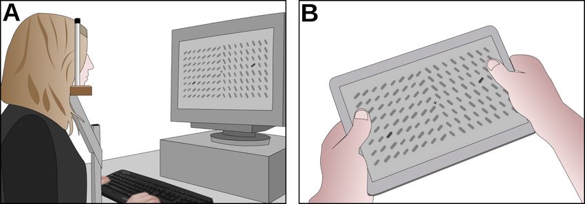
TVA in the wild |     3

assigned to every stimulus x in the visual field:
                                                       ∑︁
                                                wx =         η(x, j)π j                                        (1)
                                                       j∈R

where R represents feature categories that might be relevant in a task (e.g., colors if the task is to report, say,
blue and red objects), η(x, i) is the sensory evidence that stimulus x has feature j (e.g., medium for a pink
stimulus being red), and π is the pertinence of feature j (e.g., high for target colors blue and red and low for
other features).
      In the second wave of processing (selective wave), these weights determine how processing resources
(TVA parameter C) are distributed across the visual field, leading to a processing rate for each stimulus. This
processing rate determines if and when a stimulus is encoded in VSTM. Higher rates lead to earlier and more
certain encoding. At lower rates, stimuli proceed more slowly and are less likely to be encoded because VSTM
might be filled up before they finish processing. The VSTM capacity (TVA parameter K) is typically smaller
than four items. The formal calculation of processing rates will be explained later in section 2.2 in the context
of the present experimental paradigm.
      Summing up, TVA makes a quantitative connection between latent but theoretically interesting distinct
components of attentional processing such as attentional weights, VSTM, and processing speed. It has been
used with different experimental paradigms: whole and partial report (e.g., Bundesen and Habekost, 2008),
attentional dwell time (Petersen et al., 2013), or temporal-order judgments (Tünnermann et al., 2017). Recent
developments have been summarized by Bundesen, Vangkilde and Petersen (2015). Moreover, TVA integrates
different views, such as behavioral and neuronal interpretations of visual processing (Bundesen et al., 2005).
It is also used in the clinical context, facilitating new diagnostic applications (for a review, see Habekost,
2015).
      In the present article, we send TVA into the wild by relaxing stimulus control on the one hand and
embedding the task into game-like dynamic scenarios on the other hand as motivated above. Experiments 1, 2,
and 3 contrast a typical lab experiment with one running in a browser on mobile devices. Experiments 4, 5,
and 6 implement both factors by using a game engine and a gaming task (flying and driving a bike). One might
object that none of this releases TVA into real life or real wild. However, compared to typical psychological
experiments with their strict control, we take, to say the least, several large steps, and prepare the ground
for possible further progress. Before turning to the individual experiments, we describe the temporal-order
judgment (TOJ) paradigm, which is at the core of all experiments, in general and how exactly a model of TOJs
can be derived from TVA.

2 General Method
2.1 Experimental paradigm and relationships between the experiments

The experimental paradigm is a temporal-order judgment, an easy experimental task with a long tradition of
lab-based research (Sternberg and Knoll, 1973) in which the participants indicate which of two stimuli appears
first or, alternatively, second. Readers familiar with TVA may wonder why we did not use one of the more
common tasks such as whole and partial letter report or combiTVA (Bundesen, 1990; Vangkilde et al., 2012).
One reason is that the TOJ task is very simple and can be done by very different groups including children
(Petrini et al., 2020), animals (Wada et al., 2005) and neurophysiologically impaired persons (Rorden et al.,
1997). The other reason is that the more common TVA tasks presuppose a large set of equally recognizable
well-learned stimuli, for instance letters. The present method works with virtually any material as long as two
asynchronous stimuli can be presented.
      In the TOJ, we use a flicker instead of the more common onset of stimuli (e.g., Tünnermann, 2016) because
it is better suited for estimation of attention parameters in multi-element displays (Krüger et al., 2016). The
flicker is realized by a temporary change of the stimulus display. It is implemented by an offset and re-onset
4 | A. Krüger et al.
after a brief delay of a few hundreths of a second. The two stimuli are clearly identifiable because they are
marked by a special feature such as size or orientation, or, in one of the experiments (Experiment 6), are
pointed out to the participants as such.
The flicker of the two targets (depicted in abstract form in Figure 1) is separated by an interval that we call
SOA (stimulus onset asynchrony) which is in accordance with the TOJ literature although, strictly speaking, it
is a flicker onset asynchrony in our experiments. The range of SOAs is chosen so that the judgment accuracy of
the participants varies between chance (at an SOA of 0 ms) and few mistakes at the largest SOA.
Figure 1: Illustration of a typical TOJ task. This example sequence shows a negative SOA, at which the probe stimulus (here a
star) leads. At positive SOAs the reference (circle) would lead.
In all experiments, we increase the salience of one stimulus in an experimental condition and keep it
equal for both stimuli in a control condition. The salience boost is known to bias attention and consequently
influence processing speed and order judgments. The resulting pattern of attentional weights—balanced in
control conditions and biased in favor of attended stimuli—is well documented in laboratory experiments
(Krüger et al., 2016, 2017). Whether and to what degree this pattern can be detected “in the wild” is a research
question we address here. Even in lab settings, the distribution and activation of attentional resources likely
are subject to influences beyond the experimental stimulation. Some attention might be directed at irrelevant
parts of the apparatus (e.g., the layout of response keys), and motivation might modulate the overall resources
dedicated to correct execution of the task. Such influences might be both stronger and more diverse outside the
lab, especially when the task is embedded in less restrictive contexts. They might also work in both directions:
Motivation, for instance, could be higher, leading to more pronounced effects in less restrictive settings
while the distribution of attention over the experimentally relevant stimuli might be diluted by uncontrolled
influences of the environments. It is outside the scope of the present article to tease apart all the different
influences on attention and quantify how their impact differs between lab and “wild” settings. Instead, we are
interested in whether we can find the known patterns caused by salience-induced attention biases despite
the variable and unknown influences. The model-based estimation of meaningful attentional parameters
aids the comparison of the outcomes. However, the degree to which our experiments deviate from the typical
lab setting varies between the experiments and some include a typical lab-version of the task as a control.
We present the experiments ordered by decreasing restrictiveness and experimental control and increasing
complexity of the overall task.
In Experiments 1 to 3, we conduct—with different salience manipulations—a typical lab TOJ task both
in the lab and on an uncontrolled selection of mobile devices. While the mobile experiments retain several
aspects of the typical presentation (e.g. non-interactive one-shot trials followed by keypress responses), other
factors become less controlled (e.g., stimulus size and viewing distance, or how well web browsers on mobile
devices implement the intended timing). Experiments 4 to 6 embed the TOJ task in interactive environments.TVA in the wild | 5
Experiments 4 and 5 use games, which introduce several dynamic aspects such as changing object sizes
and positions caused by the apparent ego-motion although the experimental displays are still artificial (just
more dynamic) multi-element arrangements. Experiment 5 explores the influence of the additional factors
adaptive vs. constant gaming speed and SOA size on the attention measurements. During these experiments,
the responses are given by controlling game elements with the computer keyboard. Experiment 6 finally leaves
computer keyboards or response boxes behind and places the participants on an actual bicycle on a roller
trainer which is connected to a traffic simulation. Here participants perform TOJs by navigating the bike over
simulated objects that implement the flicker task. The objects with the experimental salience manipulation
compete with a multitude of visual influences experienced in dynamic scenes.
2.2 Formal model
How can insights on visual processing and attention be gained from TOJ data? Fitting traditional psychometric
functions (based on the logistic function or the cumulative Gaussian distribution) provides only relative latency
measures (e.g., “stimulus x is perceived as appearing 20 ms earlier than stimulus y”) and discrimination
performance measures. These components provide no direct information about how attention is distributed
across the stimuli and how fast these are processed (for instance, it cannot be distinguished whether attended
stimuli are processed faster or if unattended ones are processed slower; Tünnermann et al., 2015).
The model of TOJs used to estimate relative attentional weights and processing speed parameters from all
experiments in the present study can be derived from Bundesen’s (1990) TVA (Tünnermann et al., 2015):
According to TVA, the probability that a stimulus x is encoded until time t is given by
1 − e−v x (t−t0 )
{︃
if t > t0
F(t) = (2)
0 otherwise,
where v x is the rate with which a stimulus is encoded into VSTM and t0 is a threshold time. For presentations up
to t0 , no effective encoding occurs. In TVA, v x can be further decomposed into overall processing capacity and
relative attentional weights. We use the term “attentional weight” to refer to TVA’s relative attentional weight (cf.
Equation 3 to 8). These parameters are composed of more fine-grained ones that model pertinence (low-level
filters, e.g. “red is important, blue not”) and bias (report category biases, e.g. “letters are to be reported,
numbers must be ignored”). The formal model of how these fine-grained components produce attentional
weights can be found, for instance, in Tünnermann et al. (2015). For the present study, it is sufficient to relate
TVA’s encoding to TOJs. Assuming that temporal order is judged based on the VSTM entry order, the probability
of reporting the probe stimulus as appearing first (P p1st ) can be calculated as follows:
⎧ (︁ )︁
⎨1 − e−v p |SOA| + e−v p |SOA| v p if SOA < 0
v p +v r
P p1st (v p , v r , SOA) = (︁ )︁ (3)
−v |SOA| v
⎩e r p
v p +v r if SOA ≥ 0.
Here, v p and v r are the processing rates of the probe and reference stimuli with which they race for VSTM
encoding. The first part of the first case, for the SOAs smaller than zero (in which the probe leads), is the
probability that the probe is encoded before the reference even starts racing for VSTM (1 − e−v p |SOA| ). The
second describes the probability that this has not happened (e−v p |SOA| ) and that the probe wins the race for
VSTM when both, probe and reference, race together (v p /(v p + v r )); Luce’s choice axiom (Luce, 1977). The
second case, for SOAs larger than zero (in which the reference leads), the probability of “probe first” judgments
is e−v r |SOA| , the probability that the reference is not already encoded before the probe is shown and that the
probe wins when both race together (v p /(v p + v r )). Note that this model does not include t0 . Because t0 is
assumed to be equal for both stimuli (adding equal latencies), it cancels out in the equations (cf. Tünnermann
et al., 2015).
For the present study, it is advantageous to re-parametrize this model so that instead of individual pro-
cessing rates v p and v r the overall processing rate C and attentional weights (w*p ) can be estimated. According6 | A. Krüger et al.
to TVA, the overall processing rate C is the sum of the processing rates of the individual encodings:
∑︁ ∑︁
C= v(x, i). (4)
x∈S i∈R
Moreover, TVA states that the individual rates v(x, i) with which stimuli x are encoded into VSTM as members
of category i are calculated as
wx
v(x, i) = η(x, i)β i ∑︀ (5)
z∈S w z
where η(x, i) is the sensory evidence that stimulus x is a member of category i and β i is a bias for encoding
stimuli as members of category i. The w are attentional weights and S refers to all stimuli in the visual field. In
the following we will use v p and v r for simplicity to refer to v(p, i) and v(r, i), the rates with which probe and
reference are encoded as members of their report categories.
The experiments in the present study (in line with other TVA-based TOJ experiments) are designed so that
both η(x, i) and β i are the same for the probe and reference stimuli. That is, neither of the two has a higher η
(e.g., better visibility) nor is its report category more important (higher β) than the other. Therefore, only the
attentional weight part ( ∑︀ w x w z ) of Equation 5 is different for the two stimuli. Consequently we can assume
z∈S
that the processing rates are equal when they are divided by the attentional weights part:
wp + wr wp + wr
vp = vr (6)
wp wr
This can be rearranged to
wr
vp + vp = vr + vp (7)
wp ⏟ ⏞
C
where v p + v r (all individual processing rates) can be substituted with C (cf. Equation 4). Taking further into
account that w p + w r = 1 (because there are only two stimuli that acquire attentional weights) the equation
can be simplified to
wp
vp = C · (8)
wr + wp
⏟ ⏞
w*p
That is, the processing rates v p (and similarly v r ) in Equation 3 can be replaced by the term above. The main
benefit of this is that when fitting experiments with more than one condition, a common C can be estimated for
both conditions whereas individual w*p are estimated for each condition. Note that w*p is a relative weighting
(Tünnermann and Scharlau, 2018b; Krüger et al., 2017) that expresses the attentional advantage of the probe
stimulus relative to the attentional weighting of all modeled stimuli. For the sake of simplicity, we call w*p the
“attentional weight”. The model structure is further detailed below.
2.3 Bayesian parameter estimation
The TVA-based TOJ model derived above is embedded in a hierarchical Bayesian parameter estimation. The
model structure is depicted in Figure 2. Note that the inner structure is contained twice to model one “neutral”
condition (N) and one “salient” condition (S) in agreement with the design of most of the experiments of this
study. A common C (TVA’s overall processing rate) is estimated across the conditions. Earlier research has
shown that C remains unchanged under attentional manipulations (e.g., Krüger et al., 2016) and hence we
can pool the information about C from both conditions. However, for each condition an individual attentional
weight of the probe stimulus w*p is estimated (note that w*r , the reference’s weight can be obtained as 1 − w*p ).
For neutral conditions, w*p is expected at .5, indicating that attention is equally divided between probe and
reference. For salient conditions, w*p is expected to be larger than .5, indicating that attention is biased towards
the salient probe stimulus. As indicated in Figure 2, overall estimates of the w and C parameters are obtained
as the means of the corresponding distributions estimated for the participants.TVA in the wild | 7
C ! mean( Cj)
wpN C wpS
w N/S
p ! mean(wpN/S
j
)
Cj » Uniform(0, 250)
wpNj Cj wpSj
wpN/S » Uniform(0, 1)
j
vpjN/S ! Cj wpN/S
v pNj v rNj v pSj v rSj j
j Participants
vrjN/S ! Cj (1 wpN/S
j )
µjiN µjiS
µij
N/S
! Pp1st ( vpjN/S , vrN/S , SOAi )
i SOAs
i SOAs
j
yjiN yjiS
yjiN/S
» Binomial(p= µijN/S , N= njiN/S )
N
nji nS
ji
Figure 2: Hierarchical model structure (left) and priors and deterministic dependencies (right).
The models were implemented in pymc3 (Salvatier et al., 2016) and estimated using the NUTS sampler
(Hoffman and Gelman, 2014) with 5000 samples (in each of four chains). For attentional weights, uniform
priors with the range zero to one (equal a priori probabilities for all possible attentional weights) were used.
For the overall processing rate C a uniform range corresponding to zero to 250 Hz was used (0–0.25 items/ms).
This reflects a conservative choice, given that earlier studies found C typically around 70 Hz. Where not
indicated otherwise, estimates in the results section refer to group-level estimates obtained as means of the
participant-level posteriors. We report the full posterior distribution together with the mode (as a point estimate
of a parameter) and the boundaries of 95 % Highest Probability Density (HPD).
3 Experiment 1
In this first experiment, we move the experimental setup into the “wild” but keep the experimental paradigm
identical to typical lab-based TOJ experiments (Krüger et al., 2016, 2017). In fact, we include a within-
participants control condition performed in the usual lab setup. In the experimental condition, we have
participants perform a typical lab task in the web browsers on their own mobile devices under typical office
conditions. Why might researchers be interested in using typical tasks but collecting data “in the wild”? After
all, we are losing, at least to some degree, control over the exact circumstances under which the experiment
takes place, such as the general viewing conditions and spatial and temporal aspects of the presentations.
The use of web-based setups enables crowd-sourcing large datasets and can help to avoid WEIRD samples
(western, educated, from industrialized, rich, and democratic countries; Henrich et al., 2010). Moreover, when
researchers have no or limited access to laboratories, online experiments can be a way out. Our experiments
predated COVID-19 but certainly the pandemic led to an urgent need for online experiments in most psychology
labs.
Especially researchers who use psychophysical tasks, such as the TOJ in the focus of the present study,
typically shun away from giving up control of the most basic variables such as accurate spatial and temporal
stimulus presentation. Here, we ask whether one can still obtain useful insights from such “uncontrolled”
data. The formal model and Bayesian estimation scheme enable the estimation of meaningful parameters
and quantification of uncertainties. The rationale of Experiment 1 is to compare highly controlled lab-based
TOJ data collection with less constrained data collection to check whether under such conditions the typical
patterns can be replicated, and to assess the uncertainty of the estimates and quantify the model fit.8 | A. Krüger et al.
In this experiment, we had participants perform a typical TOJ experiment. In the experimental condition,
we increased the salience of one target whereas salience was kept balanced in neutral control trials. In a
“lab” condition, participants performed the task in a usual lab setting with controlled viewing distance to a
time-accurate CRT monitor. In the browser condition, participants used their own laptops, tablets, or mobile
phones with various display sizes and uncontrolled viewing distance. Based on earlier studies, we expect w
to be increased for a more salient target. We have no specific expectations concerning the influence of the
controlled vs. noncontrolled environment although we expect any possible changes to be at most medium (cf.
Semmelmann and Weigelt, 2017). Because we are interested to which degree the parameters from lab-based
experiment and experiments outside the lab reflect the same construct, we report their correlations.
3.1 Method
3.1.1 Participants
From earlier experiments that combined the TOJ paradigm with TVA modeling (Krüger et al., 2016, 2017),
we know that we need approximately 30 participants to reach appropriately precise parameter estimates in
experiments manipulating salience and we aimed at this number in all the experiments. Due to organizational
reasons, more participants were available in some of the experiments. Because the outcome of Bayesian
parameter estimation does not depend on sampling intentions or stopping rules (Dienes, 2011), we made use
of the opportunity to further increase precision of parameter estimation and included these participants in
the experiments and analyses.
All experiments were approved by the ethics committee of Paderborn University. Thirty-seven persons (20
male and 17 female; Mage = 24.08, range 19–62) participated. All participants were students or members
of Paderborn University. Each participant gave informed written consent, reported normal or corrected-to-
normal visual acuity and received course credit or was payed 8 Euro per hour. In the browser condition, across
all participants, 26 different combinations of devices, operating systems (and versions) and browsers (and
versions) were used. If only the major release version of operating system and browser are taken into account,
the number of different combinations is 23. Two participants completed only one instead of two sessions of the
lab condition. Because the Bayesian analysis accounts for the fact that these data sets are less informative, we
include these participants in the analysis. One participant produced no usable data set due to a configuration
problem with the monitor (see Footnote 1).
3.1.2 Apparatus
The lab condition was conducted on a Microsoft Windows 10 PC with a 22” Iiyama Vision Master Pro512
(40.4 cm × 30.3 cm) CRT monitor. A resolution of 640 × 480 pixels was used with 32-bit colors and a refresh
rate of 100 Hz. The experimental paradigm was implemented with OpenSesame (Mathôt, Shhreij & Theeuwes,
2012) and PsychoPy (Peirce, 2007). Presentation was time-synchronized with the monitor’s vertical retrace
signal. When the PC detected a mismatch between the programmed SOAs and estimates of the realized SOAs
(based on internal clock time stamps and the monitor synchronization) which was larger than 1 ms, the trial
was discarded and repeated later. Such repetition occurred on less than 0.17 % of the trials¹.
The browser condition was conducted on mobile devices the students brought to the lab, or, if they had no
working mobile device available, in the browser of a PC (Ubuntu, Firefox 70.0, 22” TFT-display, Acer V223W
Ab, with 1680 × 1050 px resolution). It was programmed using the JavaScript library jsPsych (de Leeuw, 2015).
The scripts were transpiled with Babel.js, bundled with WebPack.js, and served by JATOS (Lange, Kühn &
Filevich, 2015). Pre-loaded images were used as stimuli.
1 One participant did not finish the experiment because trials were continuously repeated due to a monitor configuration problem.TVA in the wild | 9
The same SOAs were used in both conditions. These SOAs were divisible by 10 ms which allowed accurate
presentation on the 100 Hz lab monitor. However, it was expected that most mobile devices in the browser
condition will not be able to display these SOAs accurately, fostering rather uncontrolled timing.
The viewing distance on the lab computer was 50 cm, for the browser condition it was not fixed. On the
lab computers and participants’ laptops, the Q key and the P key were used for collecting the order judgments.
On mobile devices, participants had to touch the corresponding side of the screen. The lab condition took
place in a dimly lit experimental booth, the browser condition under variable daylight conditions in an office
room.
3.1.3 Stimuli
An array of 16 × 8 bars with a fixation point in its center was shown (see Figure 3). On the lab computer, the
array encompassed 41∘ × 21∘ of visual angle. Length and width of the bars were 1.37∘ and 0.32∘ plus a small
jitter of 0.32∘ and 0.12∘ . The background color was a light gray (RGB: #c1c1c1), the bars were colored dark
gray (RGB: #7f7f7f), and the fixation mark was black. In the browser condition, the layout was the same but
sizes varied with the uncontrolled display size and viewing distances.
Figure 3: A Experimental setup in the lab condition with accurate timing on a CRT monitor, controlled viewing distance with a
head rest. B Browser condition on a mobile device with less control of stimulus timing, viewing distance and posture.
Two positions, one on the left and one on the right, contained reference and a probe stimuli. Both were
darker than the other stimuli. Depending on the condition (salient vs. nonsalient), the probe could be salient
in its orientation (90° difference from the background elements). The two positions were randomly chosen
among the inner positions in each hemifield. (The outer columns close to the screen border and the fixation
mark were excluded). Background orientation was chosen randomly in each trial (equal for all background
bars on a display half) and differed by 90∘ between the left and the right half of the display.
After the display had been presented for 300 ms plus a jitter (450 ms), probe and reference flickered
briefly by offsetting and onsetting again after 30 ms. The flickers were separated by SOAs of ±100 ms, ±70 ms,
±50 ms, ±30 ms, ±10 ms, or 0 ms. SOAs were repeated 20 times each. A video of the experiment can be found
at https://osf.io/z9h68.
3.1.4 Procedure
Participants performed in four sessions, two of the lab conditions and two of the browser conditions, in
random order. Throughout each trial, participants were instructed to fixate a point in the center of the display
that was visible from the beginning of each trial. There was no fixation control.
Observers judged which of the two flicker events appeared earlier, the event on the left or the event on the
right. Responses were given with the Q key and the P key on the computer and by touching the corresponding10 | A. Krüger et al.
half of the display on mobile devices. The next trial started automatically. A short training of 10 trials allowed
familiarization with the task. The main parts contained 440 trials and a break was offered every 44 trials. The
experiment lasted approximately 25 min.
3.2 Results and Discussion
We first report the C and w values and their difference between conditions. Afterwards, we look into correlations
for each value between the lab and the browser condition. Finally, we look at effect sizes of the salience effect
in the two conditions and compare the model fits.
We found a C difference between the lab and browser in overall capacity (see Figure 4). In the lab condition,
the mean overall processing rate C across all participants was estimated at 62.32 Hz [95 % HPD: 59.86, 64.82]
with an SD of 21.76 [95 % HPD: 19.26, 24.44]. In the browser condition, the mean overall processing rate C
across all participants was estimated at 51.91 Hz [95 % HPD: 49.60, 54.39] with an SD of 32.26 [95 % HPD:
28.16, 36.53]. The difference in C between the conditions is 10.41 Hz [95 % HPD: 6.92, 13.83].
Figure 4: Results of Experiment 1: Means for overall processing capacity, C, and attentional weight of salient and nonsalient
probe, w*p , in the lab condition, top, and the browser condition, bottom.
The overlap of the w p posterior distributions is relatively large. In the lab condition, the mean attentional
weight of the nonsalient probe across all participants was estimated at .50 [95 % HPD: .49, .51] with an SD
of 0.05 [95 % HPD: 0.04, 0.06]. The mean attentional weight of the salient probe was .53 [95 % HPD: .51, .54]
with an SD of 0.06 [95 % HPD: 0.05, 0.07]. This probe weight of the salient target is .03 higher than that of the
neutral one [95 % HPD: .01, .04].
In the browser condition, the mean attentional weight of the nonsalient probe across all participants
was estimated at .49 [95 % HPD: .48, .51] with an SD of 0.06 [95 % HPD: 0.04, 0.07] and the mean attentional
weight of the salient probe at .51 [95 % HPD: .49, .52] with an SD of 0.06 [95 % HPD: 0.05, 0.07]. The probe
weight of the attended stimulus is .01 higher than that of the neutral one [95 % HPD: .00, .03]. Comparing the
attentional weight of the salient probe between lab and browser, the difference is estimated at .02 [95 % HPD:
.00, .04].
TVA’s overall processing capacity C shows a strong positive correlation between the lab and the browser
condition supported by a very high Bayes factor (see Figure 5, left panel; posterior modes of the participant-
level estimates enter the analysis and are shown in the scatter plot). The Bayes factor (calculated with JASP,
JASP Team, 2019) quantifies how much more it is probable that the data is positively correlated than that it has
no positive correlation. Concerning w*p of the salience condition, there is no evidence in favor of a correlation
(Bayes factor below one; see Figure 5, right panel). Hence, although different in magnitude, C remains an
index of the participants’ processing capacity even under the rather uncontrolled presentation conditions.
The lack of a correlation in w*p is most likely due to the small size of the effect in the browser condition (cf.
Figure 4, lower right distribution pair) which may not be able to overrule the random fluctuations introduced
by the less controlled setting on the mobile devices.TVA in the wild | 11
Figure 5: Results of Experiment 1: The C estimates of the lab and browser session are positively correlated while no such
correlation is evident for the w*p estimates (salient probes only); BF = Bayes Factor.
To understand the difference between the same experiments in the lab and in the wild and how it may
influence the possibility to find effects known from the lab, we calculated standardized effect sizes (Cohen’s d)
for the salience effect on w*p and the probability of superiority. The latter is calculated from Cohen’s d and
gives the probability that in a random individual we measure a higher w*p in the salient condition than in the
neutral one (cf. Grisson and Kim, 2005). As Table 1 (first row) shows, effect size in the lab is larger than in the
wild. The same is true for the probability of superiority. Still, the mobile condition allows for a small effect and
a .59 superiority which might suffice for a variety of questions and when large enough samples are available.
Table 1: Effect size (ES) and probability of superiority (PS) together with their boundaries of 95 % Highest Probability Density in
the lab and wild conditions in Experiments 1 to 3.
Experiment ES w p * (lab) ES w p * (wild) PS w p * (lab) PS w p * (wild)
1 (Orientation) 0.48 [0.16, 0.84] 0.23 [-0.09, 0.54] .69 [.56, .80] .59 [.47, .71]
2 (Red–green) 1.18 [0.85, 1.55] 1.19 [0.85, 1.59] .89 [.81, .94] .89 [.81, .95]
3 (Yellow–blue) 1.54 [1.18, 1.95] 1.05 [0.74, 1.40] .95 [.89, .98] .86 [.78, .93]
The reader may be interested in how well the theoretically derived model fits the presumably more variable
data recorded “in the wild” compared to the lab recordings. Thus we provide a comparison of the goodness of
fit for Experiments 1–4 because they have a lab and “in the wild” condition. Note, first, that although we want
our model to fit the data well, we also want it to be theoretically sound which is why theory-free optimization
of model fit (e.g. by adding parameters) is no option for us. One important criterion for model fit is a visual
check. Figure A1 shows that for most participants the model curves well describe the change of data points
across SOAs. Another criterion is quantitative model fit. How to quantitatively describe and test model fits is
a very difficult question. A widely used method to analyze the model fit are posterior predictive checks that
allow for sampling of a posterior predictive p-value (Conn et al., 2018). Similar to classical p-values, the value
states the probability of observing the present or more extreme data under the fitted model. A low probability
reflects lack of fit. However, from a Bayesian perspective, the value is also a gradual indication of goodness of
fit. Values around .5 indicate good model fit (see Berkhof et al., 2000, for details). The model check requires a
discrepancy measure for which we use a χ2 measure (cf. Wichmann and Hill, 2001; Berkhof et al., 2000). We
compare the p-values in the lab and “wild” conditions separately for large and small SOAs, as more deviations
can be expected at the smaller ones, which are prone to problems in the presentation timing.12 | A. Krüger et al.
The results for the present experiment (Table 2, first row) indicate that goodness of fit is strongly reduced
in the browser condition, and it is also strongly reduced for the small SOAs. That the lowest values are
observed at smaller SOAs is in line with findings that the central parts of TOJ psychometric functions reflect
additional processes which are not included in the model we use for this study. An extensive assessment
and discussion from a TVA perspective can be found in Tünnermann and Scharlau (2018b). In the browser
condition, additional deviations are evident (both in small p-values and the subject level plots in Figure A1)
which reflect the additional noise from conducting the experiment “in the wild”. While these deviations might
be statistically strong, we believe that they do not interfere substantially with the estimation of the relevant
parameters. As can be seen in Figure A1, central deviations have little impact on the overall shape of the fitted
psychometric function.
Table 2: Posterior predictive check p-values of model fit for Experiments 1 to 4, separately for the lab and the browser condition
as well as small (Exp. 1–3: |SOA|TVA in the wild | 13
not correlate between the lab and “wild” condition. This is somewhat unexpected. However, random noise in
the individual estimates might overrule the rather small salience effect.
Effect sizes and probability of superiority are larger in the lab than in the browser condition. Model fit is
reduced in the browser condition, but the model is probably still useful. Before too strong conclusions are
drawn, we want to test the reliability of these findings. This is the purpose of Experiments 2 and 3.
4 Experiment 2
In Experiment 1, the TOJ paradigm and TVA-based modeling worked reasonably well with experiments run in
a web browser on varying and unselected (mobile) devices. However, C estimates (and to a lesser degree in
terms of distribution overlap w*p estimates) seem to be biased towards smaller values. The attention effect
on the probe attentional weight w*p was only just detectable. Experiments 2 and 3 test the reliability of this
pattern and expand the comparison to the feature dimension color which might be affected more strongly by
relaxing control than stimulus orientation.
Experiment 2 considered color salience of two colors with complementary a values in the CIELAB color
space (L = 50, a ∈ {50, −50}, b = 0). Note that a regular screen was used without color calibration and hence
the differences in LAB values only approximately adhere to the uniformity of the CIELAB color space. However,
given that colors are diametrically apart on the chromacity axes, a strong hue difference that should lead to a
relative salience effect apparent in TVA’s attentional weight parameters is guaranteed. Except for the salience
feature, the experimental procedure is the same in as Experiment 1; minor modifications are described in the
following.
4.1 Method
4.1.1 Participants
Thirty persons (9 male and 21 female; Mage = 23.41, range 19–45) participated. All participants were students
or members of Paderborn University. Each participant gave informed written consent, reported normal or
corrected-to-normal visual acuity and no color vision deficits and received course credit. All completed two
sessions in each of two conditions, except two participants, who were only available for one session in the
browser–mobile condition.
4.1.2 Apparatus
This time, both conditions used the browser-based implementation. In the browser–PC condition, the experi-
ment was run on the lab PC with the CRT monitor from Experiment 1. In the browser–mobile condition, again
the experiment was conducted on the (mobile) devices participants brought to the lab.
4.1.3 Stimuli
Stimuli were the same as in the preceding experiment, except for the following differences: The probe’s
orientation did not differ from the surrounding background bars’ orientations. All bars had the same randomly
chosen orientation and differed by 90 degrees between the left and the right side. The two targets were slightly
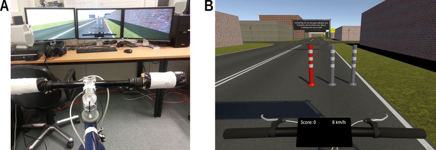
larger than the background elements in order to make them easily distinguishable as targets (see Figure 6).
Stimuli were either red (LAB: L = 50, a = 50, b = 0; RGB: #c14e79) or green (LAB: L = 50, a = −50, b = 0;
RGB: #008c75), and the probe target could be salient by having the alternative color (red among green or14 | A. Krüger et al.
green among red). The reference target always had the same color as the background elements. A video of the
experiment can be found at https://osf.io/z9h68/.
A B
Figure 6: Exemplary displays with color salience used in Experiments 2 and 3. The slightly larger line segments constitute
the probe and reference elements that flicker (separated by the stimulus onset asynchrony) to produce the temporal-order
judgment stimulation.
4.1.4 Procedure
The procedure was the same as in Experiment 1. The experiment lasted approximately 25 min.
4.2 Results and Discussion
In the browser–PC condition the mean overall processing rate C across all participants was estimated at
57.81 Hz [95 % HPD: 55.07, 60.45] with an SD of 28.81 [95 % HPD: 25.29, 32.59]. In the browser–mobile condition
the mean overall processing rate C across all participants was calculated as 34.48 Hz [95 % HPD: 32.90, 36.11]
with an SD of 16.02 [95 % HPD: 14.23, 17.71]. The difference in C is 23.33 Hz [95 % HPD: 20.22, 26.48]. In the
browser–PC condition the neutral mean attentional weight of the probe across all participants was estimated
at .50 [95 % HPD: .49, .51] with an SD of 0.05 [95 % HPD: 0.04, 0.06], and that of the salient probe at .58 [95 %
HPD: .56, .59] with an SD of 0.07 [95 % HPD: 0.06, 0.09]. The estimated weight of the salient stimulus is .08
higher than that of the neutral one [95 % HPD: .06, .09]. In the browser–mobile condition the neutral mean
attentional weight of the probe across all participants was again estimated at .50 [95 % HPD: .48, .51] with an
SD of 0.05 [95 % HPD: 0.04, 0.06], that of the salient probe at .57 [95 % HPD: .55, .58] with an SD of 0.06 [95 %
HPD: 0.05, 0.08]. The estimated weight of the salient stimulus is .07 higher than that of the neutral one [95 %
HPD: .05, .09]. Comparing the attentional weight of the salient probe between the PC and mobile conditions,
the difference is estimated at .01 [95 % HPD: -.01, .03].
The overall result pattern in Experiment 2 is very similar to Experiment 1. We found an increased attentional
weight of a salient stimulus. This is in accordance with earlier studies (Krüger et al., 2016, 2017). The increase
was very similar for the conditions run on the PC and on an unselected mobile device. Worth noting is the
difference in the parameter C. Again, C is much smaller when doing the experiment on a mobile device, and
the mean of 34 Hz is very low.
In contrast to Experiment 1, not only the C estimates but also the w*p estimates (of the salience condition)
from the browser-PC and browser-mobile condition show strong positive correlations (see Figure 8). Hence, it
seems that if a strong salience effect can be established “in the wild”, the pattern of individual differences
found in the lab can be largely reproduced.TVA in the wild | 15
Figure 7: Results of Experiment 2: Means for the overall processing capacity, C, and attentional weight of salient and non-
salient probe stimulus, w*p , in the browser–PC condition, top, and the browser–mobile condition, bottom.
Figure 8: Results of Experiment 2: As in Experiment 1, in Experiment 2 the C estimates of the browser–PC and browser–mobile
session are positively correlated; the w*p values (salient probes only) show a similar correlation in this experiment; BF = Bayes
Factor.
Effect sizes are very large, and so is probability of superiority (see Table 1, second row). What is more—and
different from Experiment 1—both effect size and probability of superiority are the same for the lab and the
mobile condition.
The model fit assessment (Table 2, second row) indicates that goodness of fit is reduced in the browser–
mobile (“wild”) condition, compared to the lab condition. It is not as low as in Experiment 1. In fact, the
browser–mobile condition seems to have a better fit than the lab condition of Experiment 1. We also point to
Appendix Figure A2 for plots of individual data and fits and the split-half reliability tests, which are reported
in Appendix Section A.6.
Because the variety of mobile devices participants bring to the lab and to further vary the salient feature,
we run another version of the experiment with other colors as Experiment 3.
5 Experiment 3
Experiment 3 is a replication of Experiment 2 with different color values (yellow and blue; LAB: L = 50, a =
0, b ∈ {50, −50}). As everything except for the color axis in the CIELAB color space was the same, we expect
the same results as in Experiment 2.16 | A. Krüger et al.
5.1 Method
5.1.1 Participants
Thirty-two persons (2 male and 30 female; Mage = 22.31, range 14–35) participated. Except for one person,
all participants were students or members of Paderborn University, gave informed written consent, reported
normal or corrected-to-normal visual acuity and no color vision deficits and, if students, received course credit.
All performed two sessions per condition, except one participant who only completed one of the browser–PC
sessions and another person who completed only one of the browser–mobile sessions.
5.1.2 Apparatus
The apparatus was the same as in the preceding experiment.
5.1.3 Stimuli
Stimuli were the same as in the preceding experiment, except for the colors which were determined setting
a = 0 and b ∈ {50, −50} in the CIELAB color space. The exact color values were #887616 (yellow; LAB:
L = 50, a = 0, b = 50) and #367ACD (blue; LAB: L = 50, a = 0, b = −50). A video of the experiment can be
found at https://osf.io/z9h68/.
5.1.4 Procedure
Procedure was the same as in Experiment 2, and the experiment again lasted approximately 25 min.
5.1.5 Results and Discussion
In the browser–PC condition, the mean overall processing rate C across all participants was estimated at
61.31 Hz [95 % HPD: 58.29, 64.24] with an SD of 34.15 [95 % HPD: 28.44, 40.53]. In the browser–mobile
condition the mean overall processing rate C across all participants was estimated at 45.27 Hz [95 % HPD:
43.09, 47.49] with an SD of 27.69 [95 % HPD: 24.27, 31.33]. The difference in C between these conditions is
16.04 Hz [95 % HPD: 12.38, 19.81].
In the browser–PC part, the neutral mean attentional weight of the probe across all participants was
estimated at .51 [95 % HPD: .49, .52] with an SD of 0.06 [95 % HPD: 0.04, 0.07], the salient weight as .60 [95 %
HPD: .59, .61] with an SD of 0.06 [95 % HPD: 0.05, 0.08]. The probe weight of the salient stimulus is .09 higher
than that of the neutral one [95 % HPD: .08, .11].
In the browser–mobile condition, the neutral mean attentional weight of the probe across all participants
was calculated as .50 [95 % HPD: .49, .51] with an SD of 0.05 [95 % HPD: 0.04, 0.06], the salient one as .57
[95 % HPD: .55, .58] with an SD of 0.07 [95 % HPD: 0.06, 0.08], with a difference of .07 [95 % HPD: .05, .08].
Comparing the attentional weights of the salient stimulus between the two browser conditions, the difference
is estimated at .03 [95 % HPD: .02, .05]. For the split-half reliability tests, see Appendix Section A.6.
The correlation of parameters estimated in the browser–PC condition and those from the browser–mobile
condition show the same pattern as in the previous experiment. While C strongly correlates, having a high Bayes
factor, the w*p correlation is weaker and much less certain (see Figure 10). The weak correlation and reduced
certainty reflected in the Bayes factor is unexpected. Experiment 3 was identical to Experiment 2, except for
the color contrast used to establish salience. We further looked into this by conducting sequence analyses
that show how evidence in favor or against the correlation accumulates when participants are iterativelyTVA in the wild | 17
added into the analysis (see Appendix Figure A8). As Appendix Figure A8C reveals, several participants do not
change the evidence level much. Nevertheless, it accumulates towards strong evidence until participant 29 is
added. Participant 29 has an exceptionally high w*p in the browser–PC condition (.76) and a very low w*p in the
browser–mobile condition (.51). A possible explanation is that rendering one of the colors (perhaps the yellow)
depended strongly on the display properties. Since no display (neither lab nor mobile) was color calibrated, it
is well possible that the colors rendered substantially different on different devices. If this was the case, it is
noteworthy that the red–green contrasts used in the previous experiment appears to be particularly robust (cf.
the correlation in Figure 10 and the corresponding sequence analysis in Figure A8B).
As in Experiment 2, effect sizes (see Table 1 are very large, and so is probability of superiority, though they
are somewhat less impressive in the wild than in the lab.
The result of the model fit (Table 2, third row) indicates that goodness of fit is reduced in the browser–
mobile condition, especially for the small SOAs. Small SOAs also show a deviation in the lab condition.
Individual data and fit plots are provided in Figure A3.
Overall, Experiment 3 confirms the pattern of results in Experiment 2. Firstly, salience results in a sub-
stantial weight increase. The increase was smaller on an unselected mobile device, but still in the range of
expected values. Again, C is strongly reduced when doing the experiment on a mobile device, and the mean of
45 Hz is comparably low. Effects sizes and probability of superiority are large.
6 Some comments on Experiments 1 to 3
We now turn to potential reasons for the substantial reduction of C in the conditions with unselected (mobile)
devices brought by the participants in Experiments 1 to 3. In general, the discrepancy could have two origins:
Participants could indeed have a reduced C available for the task on a mobile device. They might spend more
of their processing capacity on their surrounding (which is less distracting in a typical lab setup) and stimuli
occupy smaller parts of the visual field. This is in line with a reported reduction of C if the environment is
monitored for a change additionally to a concurrent task (Poth et al., 2014). However, the second possible
origin seems more likely: Many devices might not be able to present the stimuli with sufficient precision.
Especially the lower frame rate of most devices could be crucial. If at short SOAs, frames are dropped, they
can even be rendered as SOA zero (both targets start flickering in the same frame). This effectively shortens
the SOAs which lowers the precision of the order judgment and ultimately C. On the other hand, lags in
computation could lengthen SOAs depending on the exact methods of time keeping in the devices. While the
participant-level plots of conditions conducted on mobile devices generally agree with the typical data pattern
and show good fits, some indications of timing problems at the small SOAs can be seen. For instance, among
others, participant 23 of Experiment 1 shows data points clustering near .5 at smaller SOAs. At larger SOAs the
points follow the expected pattern (see Figure A1).
Figure 11 shows a comparison of the discrepancies between lab PC and unselected devices. For this purpose,
the participant-level differences from Experiments 1 to 3 in the estimates of the two conditions were grouped by
the device configuration that was used in the mobile conditions. After pooling over different version numbers,
16 configurations remained. Some contain only one or a few participants but others contained up to 27 (for
the most popular configuration “Phone / iOS / Safari”). The varying degrees of certainty in the estimates are
captured in the varying width of the distributions.
One insight of this analysis is that, different from what the results in Figure 9 suggest, the C estimates
measured with different devices vary, and some are smaller and others larger than the C estimates from the
lab condition. While C estimates are smaller on smartphones and laptops, they are increased in Windows and
Ubuntu laptops. The w*p parameters from the lab and browser condition are often similar. If they differ, the w*p
are smaller in the browser condition. While it is out of scope of the present study to investigate the technical
reasons for the implementation behaving differently on the different systems, this analysis provides a starting
point for researchers who want to run similar (timing critical) experiments on mobile devices. The mismatches
not only provide hints on where potential problems originate from (e.g. larger C: realized SOAs are too long;You can also read