Data-driven model for hydraulic fracturing design optimization: focus on building digital database and production forecast
←
→
Page content transcription
If your browser does not render page correctly, please read the page content below
Data-driven model for hydraulic fracturing design optimization: focus on building digital
                                                                       database and production forecast

                                            A.D. Morozova , D.O. Popkova , V.M. Duplyakova , R.F. Mutalovaa , A.A. Osiptsova , A.L. Vainshteina , E.V. Burnaeva , E.V. Shelb ,
                                                                                                   G.V. Paderinb
                                                                    a Skolkovo  Institute of Science and Technology (Skoltech), 3 Nobel Street, 143026, Moscow, Russian Federation
                                                               b Gazpromneft   Science & Technology Center, 75-79 liter D Moika River emb., St Petersburg, 190000, Russian Federation

                                           Abstract
                                           Growing amount of hydraulic fracturing (HF) jobs in the recent two decades resulted in a significant amount of measured data
arXiv:1910.14499v3 [eess.SY] 18 Jul 2020

                                           available for development of predictive models via machine learning (ML). In multistage fractured completions, post-fracturing
                                           production analysis (e.g., from production logging tools) reveals evidence that different stages produce very non-uniformly, and
                                           up to 30% may not be producing at all due to a combination of geomechanics and fracturing design factors. Hence, there is a
                                           significant room for improvement of current design practices. We propose a data-driven model for fracturing design optimization,
                                           where the workflow is essentially split into two stages. As a result of the first stage, the present paper summarizes the efforts into
                                           the creation of a digital database of field data from several thousands of multistage HF jobs on vertical, inclined and near-horizontal
                                           wells from circa 20 different oilfields in Western Siberia, Russia. In terms of the number of points (fracturing jobs), the present
                                           database is a rare case of a representative dataset of about 5000 data points, compared to typical databases available in the literature,
                                           comprising tens or hundreds of points at best. Each point in the data base contains the vector of 92 input variables (the reservoir,
                                           well and the frac design parameters) and the vector of production data, which is characterized by 16 parameters, including the
                                           target, cumulative oil production. The focus is made on data gathering from various sources, data preprocessing and development
                                           of the architecture of the database as well as solving the production forecast problem via ML. Data preparation has been done using
                                           various ML techniques: the problem of missing values in the database is solved with collaborative filtering for data imputation;
                                           outliers are removed using visualisation of cluster data structure by t-SNE algorithm. The production forecast problem is solved via
                                           CatBoost algorithm. Prediction capability of the model is measured with the coefficient of determination (R2 ) and reached 0.815.
                                           The inverse problem (selecting an optimum set of fracturing design parameters to maximize production) will be considered in the
                                           second part of the study to be published in another paper, along with a recommendation system for advising DESC and production
                                           stimulation engineers on an optimized fracturing design.
                                           Keywords: bridging, fracture, particle transport, viscous flow, machine learning, predictive modelling, data collection, design
                                           optimization

                                           1. Introduction and problem formulation                                           Kansas, US [72]. In 1949, first commercial treatments were ap-
                                                                                                                             plied by Halliburton Oil Well cementing Company in Texas and
                                           1.1. Introductory remarks                                                         Oklahoma, U.S. In the Soviet Union, the fracturing treatments
                                              Hydraulic fracturing (in what follows referred to as HF for                    were first performed in early 1950-s, on oil fields as well as
                                           brevity) is one of the most widely-used techniques for stim-                      for stimulation of coal bed methane production. Over the last
                                           ulation of oil and gas production from wells drilled in the                       two decades, the technical complexity of the stimulation treat-
                                           hydrocarbon-bearing formation [1]. The technology is based                        ment has made a significant step forward: wells are drilled di-
                                           on pumping at high pressures the fluid with proppant parti-                       rectionally with a near-horizontal segment and multistage frac-
                                           cles downhole through the tubing, which creates fractures in                      tured completion.
                                           the reservoir formation. The fractures filled with granular                          The global aim of this study is to structure and classify ex-
                                           material of closely packed proppant particles at higher-than-                     isting machine learning (ML) methods and to highlight the ma-
                                           ambient permeability provide conductive channels for hydro-                       jor trends for HF design optimization. Gradual development of
                                           carbons from far-field reservoir to the well all the way to sur-                  fracturing technology is based on the advances in chemistry &
                                           face. The technology of HF began in 1947 as an experiment by                      material science (fracturing fluids with programmed rheology,
                                           Stanolind Oil with gasoline as the carrier fluid and a sand from                  proppants, fibers, chemical diverters), mechanical engineering
                                           the Arkansas river at the Hugoton gas field in Grant County,                      (ball-activated sliding sleeves for accurate stimulation of se-
                                                                                                                             lected zones), and the success of fracturing stems from it be-
                                                                                                                             ing the most cost effective stimulation technique. At the same
                                               Email address: a.osiptsov@skoltech.ru (A.A. Osiptsov)                         time, fracturing may be perceived as yet not fully optimized
                                           Preprint submitted to Journal of Petroleum Science & Engineering. Special Issue: Petroleum Data Science                                      July 21, 2020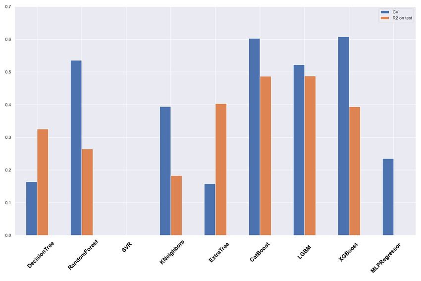
technology in terms of the ultimate production: up to 30% of             author investigated Wolfcamp well dataset. Analysis based on
fractures in a multi-stage fractured completion are not produc-          Decision Trees is applied to distinguish top quarter of wells
ing [2, 3]. For example, [4] analyzed distributed production             from the bottom quarter. Most influential subset of parameters,
logs from various stages along the near-horizontal well and con-         characterizing a well, is also selected.
cluded that almost one third of all perforation clusters are not
contributing to production. The reasons for non-uniform pro-             1.3. Prior art in frac design and its optimization
duction from various perforation clusters along horizontal wells            Typically the oilfield services industry is using numerical
in a plug-and-perf completion are ranging from reservoir het-            simulators based on the coupled solid-fluid mechanics models
erogeneity and geomechanics factors to fracturing design flaws.          for evaluation and parametric analysis of the HF job [15, 16,
Thus, the pumping schedule has yet to be optimized, and it can           17]. There is a variety of HF simulators based on KGD, PKN,
be done either through continuum mechanics modeling (com-                P3D, or Planar3D models of the hydraulic fracture propagation
mercial fracturing simulators with optimization algorithms) or           process. Shale fracturing application called for more sophisti-
via data analytics techniques applied to a digital field database.       cated approaches to modeling of the fracture network propaga-
We chose the latter route. To resolve this problem three ini-            tion. A good overview of the underlying models can be found
tial classification categories are suggested: descriptive big data       in [15, 16]. Once there is a robust forward model of the process,
analytics should answer what happened during the job, predic-            an optimization problem can be posed with a prescribed objec-
tive analytics should improve the design phase, and prescriptive         tive function [18]. Particular case of stimulation in carbonate
analytics is to mitigate production loss from unsuccessful jobs.         reservoirs is acid frac. Iranian field with 20 fractured well has
Here in Part I, we begin with the forward problem (predicting            been studied by [19] in order to test candidate selection proce-
oil production rate from HF design and reservoir geology) in             dure.
order to be able to solve the inverse problem in what follows in            A typical approach to the optimization problem includes the
Part II. The question in phase II will be posed as: what is the          construction of a surrogate (see [20]) of an objective function,
optimum design of an HF job in a multistage fracturing com-              whose evaluation involves the execution of a HF simulator. The
pletion to reach the highest possible ultimate cumulative pro-           computational model integrates a hydraulic fracture simulator
duction?                                                                 to predict propped fracture geometry and a production model to
                                                                         estimate the production flow rate. Then, an objective function is
1.2. Recent boom in shale fracturing                                     calculated, which can be any choice from papers listed in Sec-
   The boom in shale gas/shale oil fracturing owing to the si-           tion 1.3 above. An example of the realization of such optimiza-
multaneous progress in directional drilling and multistage frac-         tion strategy is presented in detail in [18]. Another example
turing has resulted in extra supply in the world oil market, turn-       of an integrated multiobjective optimization workflow is given
ing U.S. into one of the biggest suppliers. As a by-product of           in [21], which involves a coupling of the fracture geometry
the shale gas technology revolution [5], there is a large amount         module, a hydrocarbon production module and an investment-
of high-quality digital field data generated by multistage frac-         return cash flow module.
turing operations in shale formations of the U.S. Land, that fuel
the data science research into the HF design optimization [6].           1.4. ML for frac design optimization
   Modeling of shale reservoirs is a very comprehensive prob-               In North America, thanks to the great attention to multistage
lem. The flow mechanism is not yet fully understood and prop-            fracturing in shales there is an increasing amount of research
erly simulated across the industry. The full scale simulation            papers studying the application of big data analytics to the prob-
could be upgraded with ML-based pattern recognition technol-             lem of HF optimization.
ogy where maps and history-matched production profile could                 A general workflow of the data science approach to HF for
enhance prediction quality for Bakken shale [7]. Marcellus               horizontal wells implicate techniques that cluster similar crit-
shale with similar approach is detailed in [8]. Here the data            ical time-series into Frac-Classes of frac data (surface treat-
driven analytics was used instead of classical hydrodynamic              ment pressure, slurry pumping rates, proppant loading, volume
models.                                                                  of proppant pumped). Correlation of the average Frac-Classes
   Problem of activation of the natural fractures network by             with 30-day peak production is used on the second step to dis-
hydraulically-induced fractures is crucial for commercial pro-           tinguish between geographically distinct areas [22].
duction from this type of reservoirs. The mutual influence of               Statistically representative synthetic data set is used occa-
natural and artificial fractures during the job has been studied         sionally to build data-driven fracture models. The performance
by [9]. The research has predicted the fracture behavior when it         of the data-driven models is validated by comparing the results
encounters a natural fracture with the help of Artificial Neural         to a numerical model. Parameters include the size, number, lo-
Network (ANN) [10, 11, 12]. A similar approach is presented              cation, and phasing angle of perforations, fluid and proppant
in [13]. Three-level index system of reservoir properties eval-          type, rock strength, porosity, and permeability. Data-driven
uation is proposed to be a new method for gas well reservoir             predictive models (surrogate models, see [20, 23]) are gener-
model control in fractured reservoir based on fuzzy logic the-           ated by using ANN and Support Vector Machine (SVM) algo-
ory and multilevel gray correlation.                                     rithms [24]. Another approach to constructing metamodels on
   In [14] the authors developed a decision procedure to sep-            transient data (time series) is Dynamic Mode Decomposition
arate good wells from poor performers. For this purpose, the             (DMD), which is being explored, e.g., in [25].
                                                                     2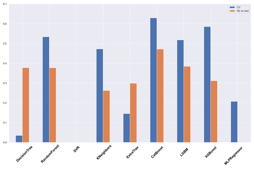
Important geomechanics parameters are Young’s modulus                      pact of geological parameters on the efficiency via classifica-
and Poisson’s ratio obtained from geomechanics lab tests on                   tion. Regression models were proposed for predicting post-
core samples, that is far away from covering full log hetero-                 frac flow rate and water cut. A portfolio of standard algo-
geneity with missing values, hence the authors used Fuzzy                     rithms was used such as decision tree, random forest, boosting,
Logic, Functional Networks and ANNs [26].                                     ANNs, linear regression and SVM. Limitations of linear regres-
   A detailed literature review on the subject of frac design opti-           sion model applied for water cut prediction were discussed. Re-
mization is provided by [27], where the authors emphasized the                cent study [35] used gradient boosting to solve the regression
necessity of bringing a common integrating approach into the                  problem for predicting the production rate after the simulation
full scale on shale gas systems. The data-driven analytics was                treatment on a data set of 270 wells. Mathematical model was
proposed as a trend in the HF design optimization. Authors                    formulated in detail, though data sources and the details of data
induced game-theoretic modeling and optimization methodolo-                   gathering and preprocessing were not discussed.
gies to address multiple issues. The impact of proppant pump-
ing schedule during the job has been investigated in [28] by                  1.5. Problem Statement
coupling fractured well simulator results and economical eval-                   To summarize the introductory remarks presented above, HF
uations.                                                                      technology is a complex process, which involves accurate plan-
   There are several approaches with different target criteria for            ning and design using multi-discipline mathematical models
optimization. For a wide variety of reasons, the proppant frac-               based on coupled solid [15] and fluid [16] mechanics. At the
tion is quite an important parameter to evaluate. In [29], the                same time, the comparison of flow rate prediction from reser-
authors reviewed four major case studies based on shale reser-                voir simulators using fracture geometry predicted by HF simu-
voirs across the U.S. and suggesting strategy to evaluate the                 lators vs. real field data suggests there is still significant uncer-
realistic conductivity and impact on stimulation economics of                 tainty in the models. The two step model of fracturing and pro-
proppant selection.                                                           duction is being extended to include the transient flowback into
   Field data, largely accumulated over the past decades, are                 the integrated optimization workflow [36], but in the present
being digitized and structured within oil companies. The mar-                 study we focus on HF design only, leaving flowback optimiza-
ket landscape in the era of declining oil prices after 2014 has               tion based on data analysis for a separate study.
stimulated shale operators to look closer at the capabilities of                 In contrast to the traditional methodology of making the de-
data science to optimize the fracturing technology [30]. The is-              sign of fracturing technology based on parametric studies with
sue of working with short-term data and the need to find a way                an HF simulator, we propose to investigate the problem of de-
to turn that into long-term well performance was emphasized.                  sign optimization using ML algorithms on field data from HF
Proppant loading was shown to be one of the most important                    jobs, including reservoir, well, frac design, and production data.
variables for productivity. Increasing industry interest to artifi-           As a training field database, we will consider the real field data
cial intelligence and to application of ML algorithms is justified            collected on fracturing jobs in Western Siberia, Russia.
by the combination of several factors: processing power growth                   The entire database from real fracturing jobs can be conven-
and amount of data available for analysis. Thousands of com-                  tionally split into the input data and the output data. The input
pletions are digitized (e.g., see [31]), giving the grounds for               data, in turn, consists of the parameters of the reservoir and the
the use of a wide range of big data analytics methods. One of                 well (permeability, porosity, hydrocarbon properties, etc.) and
the most recent studies [32] investigated the relationships be-               the frac job design parameters (pumping schedule). The output
tween the stimulation parameters and first-year oil production                is a vector of parameters characterising production.
for a database of horizontal multistage fractured wells drilled                  The usefulness of hybrid modeling is widely reported in the
in unconventional Montney formation in Canada. Four com-                      literature [37]. Numerous efforts have been made by researches
monly used supervised learning approaches including Random                    to implement data science to lab cost reduction issues. PVT cor-
Forest (RF), AdaBoost, SVM, and ANN [33] were evaluated to                    relations correction for crude oil systems were comparatively
demonstrate that the RF performs the best in terms of prediction              studied between ANN and SVM algorithms [38].
accuracy.                                                                        Finally, the problem at hand is formulated as follows: one
   The state of affairs is a bit different in other parts of the world,       may suppose that a typical hydraulically-fractured well does
where, though the wells are massively fractured, the data is not              not reach its full potential, because the fracturing design is not
readily available and is not of that high quality as in the North             optimum. Hence, a scientific question can be posed within the
America Land, which poses a known problem of “small data”                     big data analysis discipline: what is the optimum set of frac-
analysis, where neural networks do not work, and different ap-                turing design parameters, which for a given set of the reser-
proaches are called for.                                                      voir characterization-well parameters yield an optimum post-
   In Russia, there are a few attempts of using ML algorithms                 fracturing production (e.g., cumulative production over a given
to process data of HF, e.g., the paper [34] presents the results              period, say 3 months)? It is proposed to develop a ML algo-
of developing a database of 300 wells, where fracturing was                   rithm, which would allow one to determine the optimum set of
performed. Operational parameters of the treatments were not                  HF design parameters based on the analysis of the reservoir-
taken into account in this paper. Classification models were de-              well-flow rate data.
veloped to distinguish between efficient/inefficient treatments.                 Out of this study we expect also to be able to make recom-
Job success criteria were suggested in order to evaluate the im-              mendations on
                                                                          3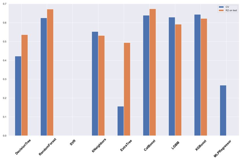
— oil production forecast based on the well and the reservoir                                Metrics                           Source
   layer data;                                                            Cumulative oil production 6/18 month
                                                                                                                                [39]
                                                                          just after the job
 — the optimum frac design;                                               12 months cumulative oil production                   [40]
                                                                          Average monthly oil production after the job          [31]
 — data acquisition systems, which are required to improve
                                                                          NPV                                                   [41]
   the quality of data analytics methods.
                                                                          Comparison to modelling                               [24]
  In the course of the study we will focus on checking the fol-           Delta of averaged Q oil                               [43]
lowing hypotheses and research questions:                                 Pikes in liquid production for 1, 3
                                                                                                                                [44]
                                                                          and 12 months
 1. Is there a systematic problem with HF design?                         Break even point (job cost equal to
 2. What is the objective function for optimization of HF de-                                                                   [34]
                                                                          total revenue after the job)
    sign? What are various metrics of success?
                                                                                           Table 1: Success metrics of HF job
 3. How do we validate the input database?
 4. What database is full (sufficient)? (Optimum ratio of num-
    ber of data points vs. number of features for the database?)           • Statistically representative set of synthetic data served as
 5. What can be learned from field data to construct a predic-               an input for ML algorithm in [24]. The study analyzed the
    tive model and to optimize the HF design?                                impact of each input parameter to the simulation results
 6. Is there a reliable ML-based methodology for finding the                 like cumulative gas production for contingent resources
    optimum set of parameters to design a successful HF job?                 like shale gas simulation model.

   At the first stage of the entire workflow, we are aimed at col-         • ∆Q = (Q2 −Q1 ) was an uplift metric to seek the re-fracture
lecting a self-consistent digital data base of several thousand              candidate for 50 wells oilfield dataset using ANN to pre-
data points (each containing infromation about the reservoir,                dict after the job oil production rate Q2 based on Q1 oil
well and frac design parameters) and solving the production                  production rate before the job [43].
forecast problem with ML methods. At the second stage, we
will consider the inverse optimization problem.                            • Q pikes approach is presented by implementing B1, B2
                                                                             and B3 statistical moving average for one, three and
1.6. Metrics of success for a fracturing job                                 twelve-month best production results consequently in
                                                                             [44]. The simulation is done over 2000 dimension dataset
  The ultimate optimization of a stimulation treatment is only               to reap the benefit from proxy modeling treatment.
possible if the outcome is measured. Below we summarize var-
ious approaches to quantify the success of an HF job:                      • Net present value is one of the metrics used to evaluate
                                                                             the success of a HF job [45]. Economical bias for HF
  • Cumulative oil production of 6 and 18 months is used by                  is detailed by [41]. The proposed sequential approach of
    [39] as a target parameter, and is predicted by a model with             integrating upstream uncertainties to NPV creates an im-
    18 input parameters, characterizing Bakken formation in                  portant tool in the identification of the crucial parameters
    North America.                                                           affecting a particular job.

  • Predictive models for the 12 months cumulative oil pro-                 In Table 1, we compose a list of the main metrics for evalua-
    duction are built by [40] using multiple input parame-               tion of HF job efficiency.
    ters characterizing well location, architecture, and com-
    pletions.
                                                                         2. Overview of ML methods used for HF optimization
  • Feed-forward neural network was used by [31] to predict
    average water production for wells drilled in Denton and                ML is a broad subfield of artificial intelligence aimed to en-
    Parker Counties, Texas, of the Barnett shale based on av-            able machines to extract patterns from data based on mathe-
    erage monthly production. The mean value was evaluated               matical statistics, numerical methods, optimization, probabil-
    using the cumulative gas produced normalized by the pro-             ity theory, discrete analysis, geometry, etc. ML tasks are the
    duction time.                                                        following: classification, regression, dimensionality reduction,
                                                                         clustering, ranking and others. Also, ML is subdivided into su-
  • In [41], a procedure was presented to optimize the fracture          pervised/unsupervised and reinforcement learning.
    treatment parameters such as fracture length, volume of                 Supervised ML problem can be formulated as constructing a
    proppant and fluids, pump rates, etc. Cost sensitivity study         target function fˆ : X → Y approximating f given a learning
    upon well and fracture parameters vs NPV as a maximiza-              sample S m = {(xm , ym )}, where xm ∈ X, ym ∈ Y with yi = f (xi ).
    tion criteria is used. Longer fractures does not necessarily            To avoid overfitting (discussed in the next section), it is
    increase NPV, a maximum discounted well revenue is ob-               also very important to select ML model properly. This choice
    served by [42].                                                      largely depends on the size, quality and nature of the data, but
                                                                     4
often without a real experiment it is very difficult to answer There are several reasons for this phenomenon [46, 47]:
which of the algorithms will be really effective.
The lack of data becomes one of the most common problems • Traditional overfitting: training a complex model on a
when dealing with field data. Some ML models can manage it small amount of data without validation. This is a fairly
(decision trees), while others are very sensitive to sparse data common problem, especially for industries that not always
(ANNs). A number of the most popular algorithms such as have access to big datasets, such as medicine, due to the
linear models or ANNs do not cope with the lack of data; SVMs difficulties with data collection.
have a large list of parameters that need to be set, and the trees • Parameter tweak overfitting: use a learning algorithm with
are prone to overfitting. many parameters. Choose the parameters based on the test
In our work, we want to show how strongly the choice of the set performance.
model and the choice of the initial sample can affect the final
results and the correct interpretation. • Bad statistics: misuse statistics to overstate confidence.
Actually, there are articles with results on application of ML Often some known-false assumptions about some system
to HF data that describe models with high predictive accuracy. are made and then excessive confidence of results is de-
However, the authors use small samples with rather homoge- rived, e.g., we use Gaussian assumption when estimating
neous data and complex models prone to overfitting. We claim confidence.
that more investigations are needed, evaluating prediction ac-
• Incomplete prediction: use an incorrectly chosen target
curacy and stability separately for different fields and types of
variable or its incorrect representation, e.g. there is a data
wells.
leak and inputs already contain target variable.
2.1. Overfitting • Human-loop overfitting: a human is still a part of the
Nowadays there exists an increasing number of papers about learning process, he/she selects hyperparameters, creates
application of ML in HF data processing. However, many stud- a database from measurements, so we should take into
ies may rise questions on the validity of results in light of po- account overfitting by the entire human/computer interac-
tential overfitting due to small data involved. tion.
Overfitting is a negative phenomenon that occurs when the • Dataset selection: purposeful use of data that is well de-
learning algorithm generates a model that provides predictions scribed by the models built. Or use an irrelevant database
mimicking a training dataset too accurately, but have very in- to represent something completely new.
accurate predictions on the test data [33]. In other words, over-
fitting is the use of models or procedures that violate the so- • Overfitting by review: if data can be collected from vari-
called Occam Razor [46]: the models include more terms and ous sources, one may select only the single source due to
variables than necessary, or use more complex approaches than economy of resources for data collection, as well as due to
required. Figure 1 shows how the pattern of learning on test computational capabilities. Thus, we consciously choose
and training datasets changes dramatically, if overfitting takes only one point of view.
place.
For example, in the article [34] only 289 wells, each de-
scribed by 178 features, were considered for the analysis. This
number of points is too small compared to the number of input
features, so a sufficiently complex predictive model simply “re-
members” the entire dataset, but it is unlikely that the model is
robust enough and can provide reliable predictions. This is also
confirmed by a very large scatter of results: the coefficient of
determination varies from 0.2 to 0.6.
In this context you can find many articles, which used small
data, of the order of 100 data points (150 wells were consid-
ered in [48], 135 wells in [8], etc.). In addition, each of the
mentioned studies uses a very limited choice of input features,
which exclude some important parameters of HF operation. For
example, the work [49] uses the following parameters to pre-
dict the quality of the HF performed: stage spacing, cemented,
number of stages, average proppant pumped, mass of liquid
pumped, maximum treatment rate, water cut, gross thickness,
oil gravity, Lower Bakken Shale TOC, Upper Bakken Shale
TOC, total vertical depth. This set of parameters does not take
into account many nuances, such as the geomechanical param-
eters of the formation or the completion parameters of the well.
Figure 1: Overfitting Quite good results were shown in [14]; various models were
5considered, but it was noted that out of 476 wells, only 171 clustering can be used for detecting outliers [55, 56] in a mul-
have records have no NaN values. tidimensional space. We utilise this for further analysis. In our
In addition to the problems described above, overfitting may case, we used t-SNE to visualize a low-dimensional structure
be caused by using too complex models: in many articles they of the data set to extract clusters and identify outlying measure-
use one of the most popular ML methods, the artificial neural ments.
network (ANN). However, it is known that a neural network is
a highly non-linear model that very poorly copes with the lack 2.4. Regression
of data and is extremely prone to overfitting. Lack of data is
a fairly frequent case when it comes to real field data, which After selecting a specific sample of data, it is necessary to
makes the use of ANNs unreliable. solve the regression problem, i.e., to restore a continuous target
There are examples of using the SVM algorithm [50]. The value y from the original input vector of features x [57, 20]. The
main disadvantage of SVM is that it has several key hyperpa- dependence of the mean value µ = f (x) of y on x is called the
rameters that need to be set correctly to achieve the best classifi- regression of y on x.
cation results for each given problem. The same hyperparame- In open literature, some authors considered different ap-
ters can be ideal for one task and not fit at all for another. There- proaches how to define a target variable. In particular, cumu-
fore, when working with SVM a lot of experiments should be lative production for 3, 6 and 12 months was taken as a target.
made, and the calculation takes a fairly large amount of time. However, we noted a strong correlation between values of cu-
Moreover, a human-loop overfitting can occur. The above algo- mulative production for 3, 6 and 12 months. Thus, as a tar-
rithms work very poorly with missing values. get variable we consider values of cumulative production for 3
In conclusion, to reduce overfitting and to construct a robust months because the production over a longer period of time is
predictive model, the necessary condition is to develop a big not always known and 3 months period is necessary and suffi-
and reliable training dataset that contains all required input fea- cient.
tures. Once the regression model is built, we assess its accuracy on
a separate test sample. As a prediction accuracy measure, we
use the coefficient of determination. The coefficient of determi-
2.2. Dimensionality reduction
nation (R2 — R-squared) is the fraction of the variance of the
When a dataset has a large number of features (large dimen- dependent variable explained by the model in question.
sion), it can lead to a large computation time and to difficulties
in finding a good solution due to excessive noise in data. In 2.5. Ensemble of models
addition, for larger feature dimension we need more examples
in the data set to construct a reliable and accurate predictive The ensemble of models [33, 10] uses several algorithms in
model. In addition, a large dimension greatly increases the like- order to obtain better prediction efficiency than could be ob-
lihood that two input points are too far away, which, like in case tained from each trained model individually.
of outliers, leads to overfitting. Therefore, in order to decrease Ensembles are very prone to overfitting due to their high
the input dimension and at the same time to keep the com- flexibility, but in practice, some assembly techniques, such as
pleteness of information with decreasing dimension, we can bagging, tend to reduce overfitting. The ensemble method is a
use special dimension reduction and manifold learning meth- more powerful tool compared to stand-alone forecasting mod-
ods, see [51, 52]. Lastly, dimensionality reduction helps visu- els, since it minimizes the influence of randomness, averaging
alizing multidimensional data. In our work, we will use the T- the errors of each basic model and reduces the variance.
distributed Stochastic Neighbor Embedding (t-SNE) algorithm
[53] for visualization after dimensionality reduction and miss- 2.6. Feature importance analysis
ing values imputation.
The use of tree-based models makes it easy to identify fea-
tures that are of zero importance, because they are not used
2.3. Clustering when calculating prediction. Thus, it is possible to gradu-
Clustering methods [33] are used to identify groups of simi- ally discard unnecessary features, until the calculation time
lar objects in multivariate datasets. In other words, our task is and the quality of the prediction becomes acceptable, while the
to select groups of objects as close as possible to each other, database does not lose its information content too much.
which will form our clusters by virtue of the similarity hypoth- There is the Boruta method [58] which is a test of the built-in
esis. The clustering belongs to the class of unsupervised learn- solutions for finding important parameters. The essence of the
ing tasks and can be used to find structures in data. Since our algorithm is that features are deleted that have a Z-measure less
database includes 23 different oilfields, horizontal and vertical than the maximum Z-measure among the added features at each
wells, as well as different types of fracture design, it would be iteration. Also, the Sobol method [59] is widely used for feature
naive to assume that data is homogeneous and can be described importance analysis. The method is based on the representation
by a single predictive model. of the function of many parameters as the sum of functions of a
Thus, by dividing dataset in clusters we can obtain more ho- smaller number of variables with special properties.
mogeneous subsamples, so that ML algorithms can easily con- In addition, testing and verifying feature importance may be
struct more accurate models on subsamples [54]. In addition, done with the one-variable-at-a-time (OVAT) method [60]. It is
6a method of creating experiments involving testing of parame- 3. Field database: structure, sources, pre-processing, sta-
ters one at a time instead of multiple factors simultaneously. It tistical properties, data mining
is primarily used when data is noisy and it is not obvious which
features affect the target. Following the report by McKinsey&Company from 2016 the
majority of companies get real profit from annually collected
data and analytics [62]. However, the main problem compa-
2.7. Hyperparameter search nies usually face while getting profit from data lies inside the
Hyperparameter optimization is the problem of choosing organizational part of the work.
a set of optimal hyperparameters for a learning algorithm. Most of the researches skip the phase of data mining, consid-
Whether the algorithm is suitable for the data directly depends ering the ready-made dataset as a starting point for ML. Never-
on hyperparameters, which directly influence overfitting or un- theless, we can get misleading conclusions from false ML pre-
derfitting. Each model requires different assumptions, weights dictions due to learning on the low-quality dataset. As follows
or training speeds for different types of data under the condi- from results of [63] the most important thing when doing the
tions of a given loss function. ML study is not only a representative sample of the wells, but
The most common method for optimizing hyperparameters also a complete set of parameters that can fully describe the
is a grid search, which simply does a full search on a manually fracture process with the required accuracy.
specified subset of the hyperparameter space of the training al- As can be seen from Section 2.1, where we describe various
gorithm. Before using the grid search, a random search can be types of overfitting, the key issue is related to poor quality of the
used to estimate the boundaries of a region, where parameters training dataset. In addition, if in case of a non-representative
are selected. Moreover, according to the Vapnik-Chervonenkis training dataset we use a subsample to train the model, corre-
theory, the more complex a model is, the worse its generalizing sponding results will be very unstable and will hide the actual
ability. Therefore, it is very important to select the model com- state of affairs.
plexity conforming to the given data set, otherwise prediction It is known that data pre-processing actually takes up to 3/4
will be unreliable. To check the generalization ability, we can of the entire time in every data-based project [64]. Having a
use a cross-validation procedure. good, high-quality and validated database is the key to obtain
the interpretable solution using ML. The database must include
all the parameters that are important from the point of view of
2.8. Uncertainty Quantification the physics of the process, be accurate in its representation and
Uncertainty comes from errors of the ML algorithm and from be verified by subject domain experts in order to avoid the in-
noise in the data set. Hence, predicting an output only is not fluence of errors in database maintenance.
sufficient to be certain with results. Therefore we should also Unfortunately, in field conditions each block of informa-
quantify uncertainty of the prediction. This can be done by us- tion about different stages of the HF is recorded in a separate
ing prediction intervals providing probabilistic upper and lower database. As a result, there is no integrated database containing
bounds on an estimate of the output variable. information about sufficient number of wells that would include
The prediction interval depends on some combination of the all factors for decision making. So, we should first develop
estimated variance of the model and the variance of the out- a correct procedure for data preprocessing in order to make a
put variable caused by noise. The variance of the model is due given data set more useful, work – more efficient, results – more
variance of model parameters estimates, resulted from noise in reliable.
the original data set. By building confidence intervals for the In the following subsections, we describe in detail the steps
parameters and propagating them through the model we can es- of forming the database, prior to applying ML algorithms. The
timate the variance of the model. In practice, to build prediction entire workflow of the study with indication of different phases
interval for a general nonlinear model we can use the bootstrap of development is shown in Figure 2.
resampling method, although it is rather computationally de-
manding [33]. 3.1. Collecting the database
Let us note that the difference between prediction and confi- We collect all necessary information from the following
dence intervals: the former quantifies the uncertainty on a sin- sources (Fig. 3):
gle observation, estimated from the population, and the latter • Frac-list — a document with a general description of the
quantifies the uncertainty on an estimated population variable, process and the main stages of loading;
such as a mean or a standard deviation. Let us note that it is
important to quantify uncertainty on ML model performance, • MPR (monthly production report) — a table with produc-
which we can do by estimating the corresponding confidence tion history data collected monthly after the final commis-
intervals. sioning;
Besides prediction or confidence intervals, another important • Operating practices — geological and technical data col-
type of uncertainty quantification is related to forward uncer- lected monthly;
tainty propagation when we estimate how the variability of in-
put parameters affects the output variance of the model. This • Geomechanics data — principal stress anisotropy, Poisson
helps to select the most important input features [59, 61]. ratio, strain modules for formations;
7Figure 2: General workflow
• PVT — a general physical properties of the fluids in the operations ended prematurely due to STOP or a screen-out are
reservoir; not necessarily tagged, making the problem more complex.
• Layer intersection data;
• Well log interpretation data.
Figure 4: Distribution of the 12 month production values
Every source from the list above was processed individu-
ally depending on the specifics before merging them with each
Figure 3: Distribution of the initial data other. Particularly, monthly data were consolidated in 3-, 6- and
12-months slices. Fig. 4 shows distribution of cumulative oil
Frac-list was selected as the key source of data due to the vol- production for 12 months (distributions for 3 and 6 months have
ume of crucial stage-by-stage data and existence of all ID keys, the same form).
such as the field, the well, the reservoir layer and the date of Some illustrative numbers of the initial database are pre-
HF operation. It is worth mentioning that the frac-list is full of sented in Table 2 and Figure 5. We show data distribution as
manually filled parameters (human errors expected). Moreover, per different oilfields, where each field is coded with a number
8Parameter Numerical value 3.2. Matching database
Observation period 2013 – 2019
When merging the data from different sources, there is often
Number of oil fields 23 a lack of a uniform template for different databases. To resolve
Number of wells 5425 this issue, we used regular expression algorithms and morpho-
– vertical & directional 4111 logical analysis to identify typos. This approach allowed us to
– horizontal 1314 automate the process of data preparation and to make it rigor-
Number of fracturing operations 6687 ous.
– single-stage treatment 3177 To isolate typos that are inevitable in large databases, which
– multi-stage treatment 3510 are filled by different individuals, we created “dictionaries” for
– refracturing operations (out of total) 2431 all sorts of categorical variables (features). With the help of the
Number of STOPs (e.g. screenout) 797 Levenshtein distance [65] we found the word analogues that
were considered equal. Since the “dictionary” we used was not
Initial number of input parameters 296
very large, we applied the brute-force search strategy, which
Final x vector of input parameters 92
showed high efficiency.
– formation 36
Figure 6 shows the structure of database and its sources.
– well 12
– frac design 44
Number of production parameters 16 3.3. Rounding/Averaging the values within database
Some data sources, such as well logs, appear in a raw format,
Table 2: Statistics of the database where parameters (permeability, porosity, etc.) are defined for
each small interval (of the length ≈ 0.3 m) all over the entire
length of a well, where measurements were taken. Such param-
(we avoid specific oilfield names for confidentiality reasons, in eters need some averaging as we need them single-valued for
agreement with the operator). It is worth mentioning that the each well.
word operation (in legend and tables) refers to the entire stim- Averaging of these features can be handled as follows:
ulation treatment, which may be a single stage fracturing on
a vertical well or a multi-stage fracturing on a near-horizontal • Porosity, permeability, clay content, oil saturation: aver-
well. Then, a multi-stage treatment (operation) is divided into age and mean per perforation interval and over the layer;
different stages. Each stage is characterized by the set of frac
• kh: mean per perforation and layer;
design parameters, but the transient pumping schedule within
an individual stage is not (yet) considered in the present study. • NTG: the total amount of pay footage divided by the total
Also, the entire treatment on the layer could be repeated after thickness of the interval for perforation and layer;
a while in order to increase oil production, i.e. refracturing op-
eration. According to data, fracturing treatment may be carried • Stratification factor: number of impermeable intervals per
out up to five times on some wells. Thus, 36% of total number layer and perforation.
operations has production history before the entire treatment. For these parameters, there is a limitation in accuracy, de-
fined by the precision of typical well logging, which is about
30cm (hence, for determining the stratification factor one can-
not detect an impermeable interval below this threshold).
As for the case of multi-stage fracturing, fluid, proppant,
breaker amounts and fracture parameters (width, length and
height) were summed up, and other parameters were averaged.
In some cases, a well has multiple perforation intervals at dif-
ferent layers (multilateral wells, for example). There are pro-
duction reports for every layer, distributed by its net pay. In
these cases, we summarise the data from different layers (as the
measurements are conducted along the entire well).
3.4. Database cleanup
For categorical features, we can mainly restore actual values
in case of typos, whereas this is not always the case for real-
valued features. Also very sensitive sensors (in logging) can
show several values (or range of values) for a certain interval,
and all of them are recorded as a characteristic for a given in-
Figure 5: Distribution of wells by oilfields
terval (for example, 1000-2000). However, in our database we
need single-valued parameters.
9As a result, we delete erroneous and uncharacteristic val- This approach allows one to indirectly save the name and size
ues: instead of magnitudes that were informational noise (e.g., of the proppant. Thus, the binary space dimension of categori-
a string value in a numeric parameter) a Not-a-Number value cal features increases only up to 257, which allowed us to speed
(NaN) was used. For features values, initially represented by up training of the ML model and to improve overall prediction
ranges, corresponding average values were used in order to accuracy.
make them unambiguous and at the same time not to add ex-
tra noise to the dataset. In order to keep our feature values in a 3.6. Handling outliers
confident range we used an expert opinion on the final compila- Outliers, i.e. objects that are very different from the most
tions. For each parameter, we had a continuous exchange with of observations in the data set, often introduce additional noise
a corresponding expert in field data working with the operator to an ML algorithm [55]. Outliers can be classified into three
to crosscheck specific margins for each a zone of interest: field, types: data errors (measurement inaccuracies, rounding, incor-
formation, pad, well. rect records), which occur especially often in case of field data;
the presence of noise in objects descriptions; suspiciously good
or bad wells; the presence of objects from other populations,
e.g., corresponding to significantly different field geologies.
To effectively detect such observations we used several tech-
niques. First of all, we used statistical methods to analyse data
distribution along different dimensions and detected outliers by
estimating the kurtosis measure and other statistics.
Secondly, we used clustering. Clustering was carried out
using the Density-based spatial clustering of applications with
noise (DBSCAN) algorithm [68], because it does not require
an a priori number of clusters to be specified in advance, and
is able to find clusters of arbitrary shape, even completely sur-
rounded, but not connected. Even more importantly, DBSCAN
is quite robust to outliers. As a result, outliers are concentrated
in small blobs of observations.
Another method that eliminated more than a hundred ques-
tionable values was an anomaly detection method called Isola-
tion Forest [69], which is a variation of a random forest. The
idea of the algorithm is that outliers fall into the leaves in the
early stages of a tree branching and can be isolated from the
main data sample.
3.7. Filling missing values (NaNs)
It is very often that certain features of some objects of the
field data sets are absent or corrupted. Moreover, many of
ML algorithms like SVM regression or ANNs require all fea-
ture values to be known. Considering the structure of the data
sources, we could expect that the frac-list has contributed to the
majority of such cases of data incompleteness, since this doc-
ument contains most of the useful data yet it is typically filled
in manually, hence it is highly dependent on the quality of the
Figure 6: Block diagram of the database creation filling process (Fig. 3 & Fig. 7).
As a result there is a number of methods that allow one to
fill in the missing values. However, it should also be noted that
3.5. Categorical features most approaches can be overly artificial and may not improve
the final quality.
In the entire database, the number of categorical features is We test several approaches to fill in missing values within the
equal to 22. If we use one-hot encoding [66] for each unique framework of the regression problem under consideration:
value of each input categorical feature, the feature space is ex-
panded with 3188 additional binary features. This leads to the • dropping objects containing more NaNs within an object
curse of dimensionality problem [67], and, obviously, increases (j-th row of a matrix representing the data set) than a cer-
the calculation time and risk of overfitting. Therefore, for cat- tain threshold (65%). For example, if a well has 33 miss-
egorical features, which usually denote the name of the prop- ing feature values out of 50, then we drop it. Among other
pant for HF, we left the main name of the manufacturer and the imputation methods described below, this would keep the
number of the stage in which this particular proppant was used. database as original as possible;
10• filling NaNs of i-th parameter by the average for the wells Comparison between different ML algorithms with these filling
in a well cluster, that are grouped by geography. The rea- methods can be seen in Figs. 16, 17, 18 and 19. Matrix fac-
son for selecting this method of filling in is that the wells torization appeared to be the most effective method, so it was
of the same cluster have similar frac designs and geology applied to the entire dataset. Handling negative values (skin-
properties of the reservoir layer; factor) has been done via introducing a binary parameter, which
shows whether the skin is negative or not.
• filling missing values by applying imputation via collabo- Then, several ML models were chosen to predict cumulative
rative filtering (CF) [70]. CF is a technique used by recom- oil production over 3 months. The target function distribution
mender systems, which makes prediction of absent values is shown in Fig. 4.
with the use of mathematical methods. According to our The following ML regression algorithms were used: SVM,
research, the best results were shown by non-negative ma- KNN, ANN, Decision Trees, and various types of ensembles
trix factorization (NNMF) and truncated singular value de- based on decision trees such as Random Forest, ExtraTrees,
composition (TSVD). Worth noting, NNMF cannot handle CatBoost, LGBM and XGBoost.
negative values, such as skin-factor. Each model was trained on a subsample with cross validation
on 5 folds. Then, models were tested on a separate (hold-out)
• applying unsupervised learning to define similarity clus-
sample. All these sets were shuffled and had similar target value
ters and filling NaNs of i-th parameter by the mean of the
distributions. Most of the ML models are decision tree-based
cluster. In other words, the average of the feature is taken
and, hence, have important advantages: they are fast, able to
not from the entire database, but from the cluster, which
work with any number of objects and features (including cate-
allows us to estimate the missing value more accurately.
gorical ones), can process data sets with NaNs and have a small
number of hyperparameters.
Each experiment is conducted two times on four data sets
constructed using different imputation techniques:
• on the entire dataset containing information about 5425
wells. Here, we used hyperparameters of the regression
algorithms set to their default values first. Then, after fig-
uring out the best imputation technique, we proceed to the
next experimental setup described below;
• on wells from one field only; again, we used default hy-
perparameters of the regression algorithms.
The reason to use two experimental setups is to check if more
homogeneous data set enhances predictive performance of the
model.
Figure 7: Distribution of missing values
Then, we take the best performing methods based on the R2
on test set of each experiment, tune their hyperparameters via
the grid search, and combine them into an ensemble to further
4. ML algorithms implemented in the present work improve the results. If the result of the ensemble of models
is worse than the single best regressor, then we are taking the
results of the best regressor.
4.1. Regression
Once the database is created, four imputation methods of fill-
4.2. Feature analysis
ing NaNs are evaluated in terms of their performance. After
applying these imputation methods to the database, the results
Feature importance analysis is performed for an ensemble of
of the best tuned ML algorithms for regression problem are as
the best algorithms. OVAT analysis is carried out to see how
follows (R2 ):
the target varies with the variation of the design parameters. In
• Matrix factorization: R2 = 0.773; addition, if the feature rankings of both methods are more or
less similar, then we may proceed to parameter reduction. With
• Dropping the entire row, if NaN’s count more than 65% in the available feature importance values, we iterate over a range
that row: R2 = 0.688; to remove less important parameters and then calculate the R2
score. This procedure is important for the design optimization
• Filling with mean values of the well pad: R2 = 0.607; (which would be considered in the second psrt of this research
in another article), because it reduces the dimensionality of the
• Filling with mean values of the cluster: R2 = 0.577. problem while keeping the best score.
114.3. Uncertainty Quantification • The family of decision-tree based algorithms show bet-
ter accuracy than other approaches. CatBoost algorithm
Finally, uncertainty quantification is done for the model met-
(based on gradient boosted decision trees) outperforms all
ric (the determination coefficient R2 ) by running the model mul-
other methods;
tiple times for different bootstrapped samples. We can repre-
sent a result of this step in the following form: 95% probability
• Some of the ML algorithms like SVM and ANN resulted
chance that the value of R2 is located within the given interval.
in negative R2 , which is interpreted as poor prediction ac-
The scheme of the forward problem methodology is depicted
curacy. The possible explanation is that both methods are
on Fig. 15 (see Appendix).
preferred when there are homogeneous/hierarchical fea-
tures like images, text, or audio, which is not our case;
5. Results and Discussion
• The best imputation technique is collaborative filtering;
5.1. Filling missing values and clustering
• Based on the log scale regression plot, a relatively large
By applying the first method of missing data imputation, we amount of errors comes from the points with too low or
droppped the rows with more than 42 NaNs. Then, the rest of too high oil production rates. The possible solution of the
the NaNs for other objects in the data set are filled with their problem is to perform regression for different clusters;
mean values.
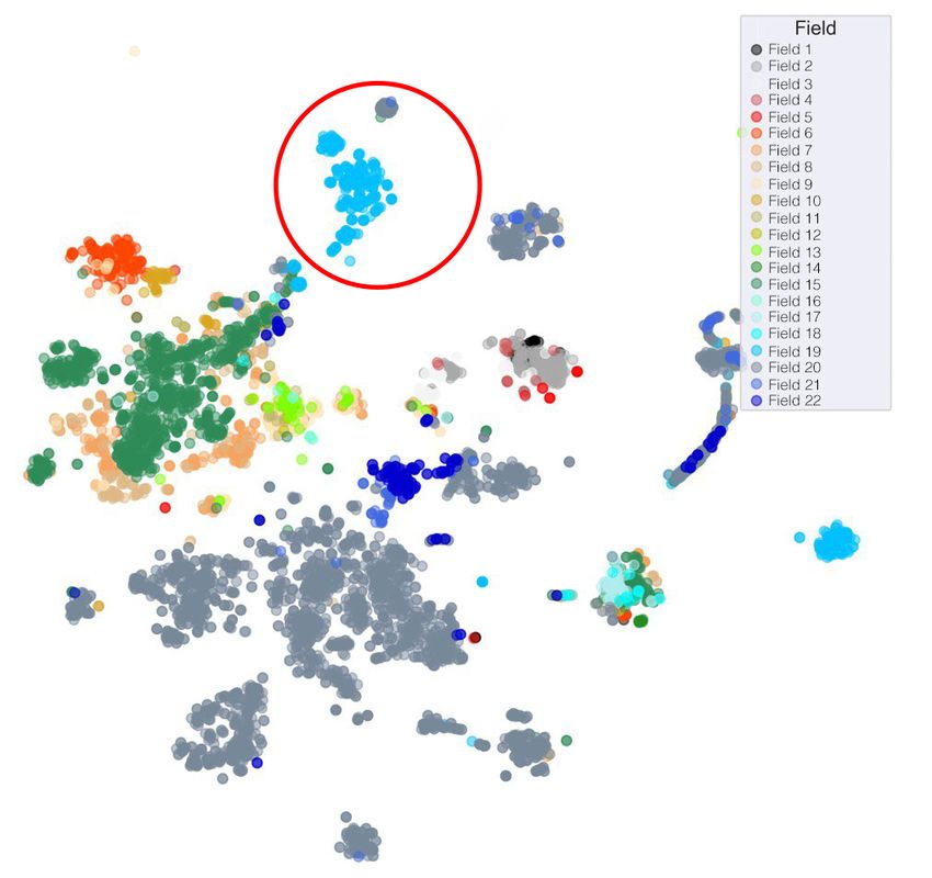
Fig. 8 shows how the entire database is clustered with DB- • Once the imputed dataset was split into 3 clusters, we
SCAN algorithm. Since the algorithm itself cannot handle found out that cluster “0” and “3” contain a relatively small
missing values, we recover them using the collaborative filter- amount of samples (∼ 800 wells). Therefore, it has be-
ing. Then we assign cluster labels for each well to the original come evident that if we construct a separate predictive
data set. To visualize clusters, t-SNE is applied to transform model on each cluster this can result in overfitting even
data space into 2D and build a scatter plot. As seen from the fig- with a simple model (KNN). Thus, the test R2 score ap-
ure, there are 3 groups in total with the biggest cluster marked pears to be 0.750 for both clusters. For the largest clus-
as “2” ter (number 2), which contains 1844 objects, the R2 test
score reached values higher than 0.850, and the overall R2
is 0.8, which is less than for the model trained on the whole
dataset.
5.3. Hyperparameter search and ensemble of models
Since CatBoost performs better than other boosting algo-
rithms and itself is an ensemble model, there is no need to cre-
ate ensemble of models. What needs to be done is to tune the
model to achieve higher score. Since our model is overfitting,
it is necessary to regularize it. With the help of grid search,
we iterate over values of the L2 regularization of the CatBoost
ranging from 0 to 2 with a 0.1 step. The tree depth is ranging
from 2 to 16. These hyperparameters have the highest impact
on the overall test R2 .
Below is the list of optimal hyperparameters, for which the
final accuracy is 0.815 on the test set for target (Fig. 9) and
0.771 (after exponentiating) for target logarithm (Fig. 10):
• depth = 7;
Figure 8: t-SNE visualization plot of the whole database for imputing NaNs by
• l2 leaf reg = 0.6;
clusters
• learning rate = 0.02;
• od type = ’Iter’ – the overfitting detector, the model stops
5.2. Regression
the training earlier than the training parameters enact;
The results of the four imputation methods on the entire
database are shown in Appendix. The R2 is calculated for the • od wait = 5 – the number of iterations to continue the train-
test sample for 9 regression algorithms. ing after the iteration with the optimal metric value.
We can see that:
12You can also read