2013 FORECASTING METHODOLOGY INFORMATION PAPER - National Electricity Forecasting - AEMO

2013
FORECASTING
METHODOLOGY
INFORMATION PAPER
National Electricity Forecasting

Published by

AEMO
Australian Energy Market Operator
ABN 94 072 010 327

Copyright © 2013 AEMO

© AEMO 2013

FORECASTING METHODOLOGY INFORMATION PAPER

Disclaimer
This publication has been prepared by the Australian Energy Market Operator Limited (AEMO) as part of a series
of information papers about the development of AEMO’s demand forecasts for the National Electricity Market for
2012-13 onwards, to be used for AEMO’s planning and operational functions under the National Electricity Rules.

This publication may contain data provided by or collected from third parties, and conclusions, opinions,
assumptions or forecasts that are based on that data. AEMO does not warrant or represent that the information in
this publication (including statements, opinions, forecasts and third party data) is accurate, complete or current, or
that it may be relied on for any particular purpose.

Anyone proposing to rely on or use any information in this publication should independently verify and check its
accuracy, completeness, reliability and suitability for purpose, and should obtain independent and specific advice
from appropriate experts.

To the maximum extent permitted by law, neither AEMO, nor any of AEMO’s advisers, consultants or other
contributors to this publication (or their respective associated companies, businesses, partners, directors, officers
or employees) shall have any liability (however arising) for any information or other matter contained in or derived
from, or for any omission from, this publication, or for a person’s use of or reliance on that information.

Copyright Notice
© 2013 - Australian Energy Market Operator Ltd. This publication is protected by copyright and may be used
provided appropriate acknowledgement of the source is published as well.

Acknowledgements
AEMO acknowledges the support, co-operation and contribution of all participants in providing the data and
information used in this publication.

ii Introduction © AEMO 2013

[This page is left blank intentionally]

© AEMO 2013 Introduction iii

FORECASTING METHODOLOGY INFORMATION PAPER

ABOUT THIS INFORMATION PAPER
The 2013 Forecasting Methodology Information Paper is a companion document to the 2013 National Electricity
Forecasting Report (NEFR). It is designed to assist in interpreting the electricity demand forecasts contained
in the NEFR.

This paper provides a detailed description of how the 2013 annual energy and maximum demand forecasts were
developed. It outlines how AEMO sought to ensure the forecasting processes and assumptions were consistently
applied and fit for purpose. It details the modelling improvements made to the forecasts compared to the 2012
report, following detailed analysis.

In addition to explaining the methodology behind the demand forecasts, this paper provides further detail on the
electricity demand segments featured in the 2013 NEFR and the approaches used to develop the forecasts for
each forecasting component.

Key improvements include:

 • The inclusion of the short-term focus (one-to-five-years) in the annual energy models.

 • The inclusion of weather adjustments and allowing for the expected use of appliances at peak times in
 maximum demand models.

 • A direct approach to gathering operational data from large industrial customers and transmission network
 service providers (TNSPs) or distribution network service providers (DNSPs) in developing large industrial
 load forecasts.

 • Inclusion of additional data for historical estimates and payback periods as the basis for installed capacity
 forecasts for rooftop photovoltaic (PV) uptake.

 • Increased transparency of the forecast approach and results, with the inclusion of Commonwealth
 Government initiatives and building standards for energy efficiency offsets.

 • A revised methodology for the development of forecasts for existing and possible future small non-
 scheduled generation plant.

The modelling and forecasting methodology processes for each component have been endorsed and approved by
both AEMO’s subject matter experts and external reviewers. Reviewers include AEMO’s advisor Woodhall
Investment Research, and independent peer reviewer, Frontier Economics.

iv Introduction © AEMO 2013

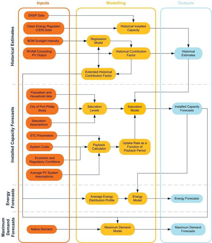
CONTENTS
ABOUT THIS INFORMATION PAPER IV
CHAPTER 1 - INTRODUCTION 1-1
1.1 National electricity forecasting 1-1
1.2 Content of paper 1-1

CHAPTER 2 - RESIDENTIAL AND COMMERCIAL LOAD 2-3
2.1 Annual energy 2-3
 2.1.1 Annual energy models 2-4
 2.1.2 Modelling approach 2-8
 2.1.3 New South Wales 2-17
 2.1.4 Queensland 2-17
 2.1.5 Victoria 2-18
 2.1.6 South Australia 2-19
 2.1.7 Tasmania 2-20
2.2 Maximum demand 2-21
 2.2.1 Maximum demand model 2-22
 2.2.2 Simulation of maximum demand distribution 2-24
 2.2.3 Changes from 2012 2-24

CHAPTER 3 - LARGE INDUSTRIAL LOAD 3-25
3.1 Forecasting large industrial load 3-25
3.2 Approach used for the 2013 NEFR 3-25
3.3 Changes from the 2012 methodology 3-26

CHAPTER 4 - ROOFTOP PHOTOVOLTAIC 4-29
4.1 Introduction 4-29
4.2 Rooftop PV scenarios 4-31
4.3 Historical estimates 4-31
 4.3.1 Historical rooftop PV contribution factor 4-32
 4.3.2 Historical installed capacity 4-34
 4.3.3 Adjustment of 2012 historical installed capacity 4-34
4.4 Installed capacity forecast 4-34
 4.4.1 Modelling the payback period 4-34
 4.4.2 Modelling the uptake rate as a function of the payback period 4-35
 4.4.3 Estimating saturation levels 4-37
 4.4.4 Application of saturation levels to installed capacity forecasts 4-38
 4.4.5 Barriers to uptake 4-38
4.5 Rooftop PV energy forecasts 4-38
 4.5.1 Adjustment of results against actual data 4-39
4.6 Rooftop PV contribution to maximum demand 4-40
4.7 Changes from the 2012 methodology 4-40

© AEMO 2013 Contents v

FORECASTING METHODOLOGY INFORMATION PAPER

CHAPTER 5 - ENERGY EFFICIENCY 5-42
5.1 Introduction 5-42
5.2 Energy efficiency uptake scenarios 5-45
5.3 Savings from energy efficiency policy measures 5-45
 5.3.1 Equipment energy efficiency savings 5-46
 5.3.2 Building energy efficiency savings 5-47
5.4 Calculating the NEFR energy efficiency forecast for annual energy 5-47
5.5 Calculating the NEFR energy efficiency forecasts for maximum demand 5-50
5.6 Modelling limitations and exclusions 5-50
5.7 Changes from the 2012 methodology 5-51

CHAPTER 6 - SMALL NON-SCHEDULED GENERATION 6-52
6.1 Introduction 6-52
6.2 Small non-scheduled generation scenarios 6-52
6.3 Calculating the NEFR small non-scheduled demand forecast for annual energy 6-52
6.4 Calculating the NEFR small non-scheduled demand forecast for contribution to maximum
 demand 6-53
6.5 Modelling limitations and exclusions 6-53
6.6 Changes from the 2012 methodology 6-54

CHAPTER 7 - DEMAND-SIDE PARTICIPATION 7-55
7.1 Introduction 7-55
7.2 DSP methodology 7-55
7.3 Estimate of current DSP from large industrial loads 7-55
7.4 Estimate of current DSP from smaller loads 7-58
7.5 The combined DSP forecast for 2013-14 7-58
 7.5.1 Seasonal data 7-58
 7.5.2 Different price levels 7-58
 7.5.3 Probability of exceedence maximum demand forecasts 7-59
7.6 Assumed growth of DSP in the future 7-59
7.7 Modelling limitations and exclusions 7-59
7.8 Changes from the 2012 methodology 7-60

APPENDIX A - INPUT DATA, CHANGES AND ESTIMATED
 COMPONENTS A-1
A.1 Changes to historical data A-1
 A.1.1 All NEM regions A-1
 A.1.2 New South Wales A-1
 A.1.3 Queensland A-2
 A.1.4 Victoria A-2
 A.1.5 South Australia A-2
 A.1.6 Tasmania A-2
A.2 Estimated components for the forecasts A-2
 A.2.1 Transmission loss forecasts A-2
 A.2.2 Auxiliary loads forecast A-3

vi Contents © AEMO 2013

APPENDIX B - ROOFTOP PHOTOVOLTAIC FORECAST B-6
B.1 Annual energy B-6
B.2 Maximum demand B-7

APPENDIX C - ENERGY EFFICIENCY FORECAST C-9
C.1 Annual energy C-9
C.2 Maximum demand C-10

APPENDIX D - DEMAND-SIDE PARTICIPATION FORECAST D-12
D.1 Estimate of current DSP capacity D-12
D.2 Queensland DSP to 2032–33 D-13
D.3 New South Wales (incl. ACT) DSP to 2032–33 D-14
D.4 Victorian DSP to 2032–33 D-15
D.5 South Australian DSP to 2032–33 D-16
D.6 Tasmanian DSP to 2032–33 D-17

APPENDIX E - GENERATORS INCLUDED E-18
E.1 Queensland E-18
 E.1.1 Power stations used for operational demand forecasts for Queensland E-18
 E.1.2 Power stations used for annual energy forecasts for Queensland E-19
E.2 New South Wales E-20
 E.2.1 Power stations used for operational demand forecasts for New South Wales (including ACT) E-20
 E.2.2 Power stations used for annual energy forecasts for New South Wales (including ACT) E-21
E.3 South Australia E-23
 E.3.1 Power stations used for operational demand forecasts for South Australia E-23
 E.3.2 Power stations used for annual energy forecasts for South Australia E-24
E.4 Victoria E-25
 E.4.1 Power stations used for operational demand forecasts for Victoria E-25
 E.4.2 Power stations used for annual energy forecasts for Victoria E-26
E.5 Tasmania E-27
 E.5.1 Power stations used for operational demand forecasts for Tasmania E-27
 E.5.2 Power stations used for annual energy forecasts for Tasmania E-28

© AEMO 2013 Contents vii

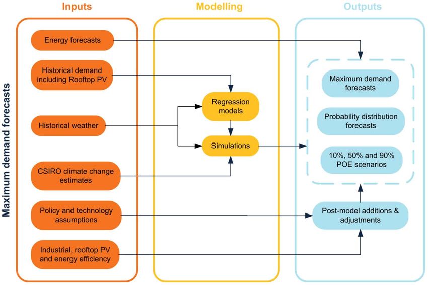
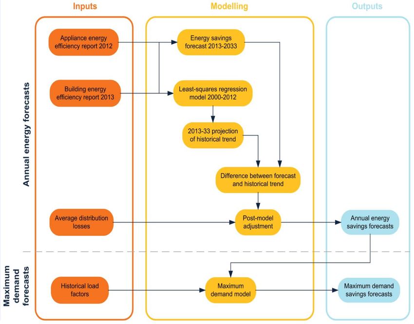
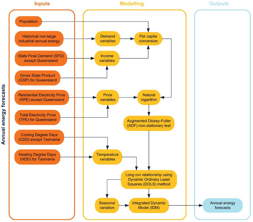
FORECASTING METHODOLOGY INFORMATION PAPER

TABLES
Table 1-1 — 2013 NEFR scenario mapping 1-1
Table 2-1 — Final variable selection 2-7
Table 2-2 — ADF tests, constant with linear trend 2-8
Table 2-3 — Estimated long-run income and price elasticities 2-9
Table 4-1 — Drivers and mapping of rooftop PV scenarios 4-31
Table 4-2 — Payback period calculator parameters and assumptions 4-35
Table 5-1 — Estimated distribution losses in Australia (% of transmitted energy) 5-49
Table 5-2 — Regional load factors for maximum demand savings assessment 5-50
Table A-1 — Historical transmission losses as a percentage of industrial and non-large industrial consumption A-3
Table A-2 — Auxiliary loads expected percentages for the annual energy demand forecasts A-3
Table A-3 — Auxiliary loads expected percentages for the summer maximum demand forecasts A-4
Table A-4 — Auxiliary loads expected percentages for the summer maximum demand forecasts A-5
Table B-1 — Post-model adjustments by state for each scenario (GWh/year) B-7
Table B-2 — Post-model adjustment to summer maximum demand forecast (MW) B-7
Table B-3 — Post-model adjustment to winter maximum demand forecast (MW) B-8
Table C-1 — Post-model adjustments by state for each scenario (GWh/year) C-10
Table C-2 — Post-model adjustment to summer maximum demand forecast (MW) C-10
Table C-3 — Post-model adjustment to winter maximum demand forecast (MW) C-11
Table D-1 — Expected DSP (MW), winter 2013 D-12
Table D-2 — Expected DSP (MW), summer 2013–14 D-12

FIGURES
Figure 2-1 — Annual energy forecasts diagram 2-4
Figure 2-2 — Long-run residuals for Queensland 2-10
Figure 2-3 — Long-run residuals for New South Wales 2-11
Figure 2-4 — Long-run residuals for South Australia 2-11
Figure 2-5 — Long-run residuals for Victoria 2-12
Figure 2-6 — Long-run residuals for Tasmania 2-12
Figure 2-7 — Regional response to permanent 1% increase in income 2-15
Figure 2-8 — Regional response to permanent 1% increase in electricity prices 2-16
Figure 2-9 — Maximum demand forecasts diagram 2-22
Figure 4-1 — Rooftop PV forecast diagram 4-30
Figure 4-2 — Historical contribution factor process 4-33
Figure 4-3 — Uptake rate as a function of payback period 4-36
Figure 4-4 — Sample of actual power and energy 4-39
Figure 5-1 — Energy Efficiency forecasts diagram 5-42
Figure 5-2 — Drivers of change in energy consumption 5-43
Figure 5-3 — Scope of energy efficiency forecasts 5-44
Figure 5-4 — Appliance/equipment energy efficiency projected savings – E3 modelling categories 5-46
Figure 5-5 — Building stock energy efficiency projected savings 5-47
Figure 5-6 — Energy efficiency forecasts for equipment energy efficiency measures 5-48
Figure 5-7 — Energy efficiency forecasts for building stock energy efficiency measures 5-49
Figure 7-1 — Time of day with prices above $1000/MWh in Victoria (Jan 2002 – Mar 2013) 7-56
Figure 7-2 — Probability of DSP response in NSW based on historical responses (Jan 2002 - Mar 2013) 7-57
Figure B-1 — Post-model adjustments by scenario measured at transmission level B-6
Figure C-1— Post-model adjustments by scenario measured at transmission level C-9
Figure D-1 — Assumed DSP growth in Queensland, winter D-13

viii Contents © AEMO 2013

Figure D-2 — Assumed DSP growth in Queensland, summer D-13
Figure D-3 — Assumed DSP growth in New South Wales (incl. ACT), winter D-14
Figure D-4 — Assumed DSP growth in New South Wales (incl. ACT), summer D-14
Figure D-5 — Assumed DSP growth in Victoria, winter D-15
Figure D-6 — Assumed DSP growth in Victoria, summer D-15
Figure D-7 — Assumed DSP growth in South Australia, winter D-16
Figure D-8 — Assumed DSP growth in South Australia, summer D-16
Figure D-9 — Assumed DSP growth in Tasmania, winter D-17
Figure D-10 — Assumed DSP growth in Tasmania, summer D-17

EQUATIONS
Equation 2-1 — Dynamic Ordinary Least Squares 2-5
Equation 2-2 — Error Correction Model with long-run estimates 2-6
Equation 2-3 — Integrated Dynamic Model 2-14
Equation 2-4 — New South Wales long-run DOLS 2-17
Equation 2-5 — New South Wales EC term 2-17
Equation 2-6 — New South Wales non-large industrial consumption forecasting model 2-17
Equation 2-7 — Queensland long-run DOLS 2-18
Equation 2-8 — Queensland EC term 2-18
Equation 2-9 — Queensland non-large industrial consumption forecasting model 2-18
Equation 2-10 — Victoria long-run DOLS 2-18
Equation 2-11 — Victoria EC term 2-19
Equation 2-12 — Victoria non-large industrial consumption forecasting model 2-19
Equation 2-13 — South Australia long-run DOLS 2-19
Equation 2-14 — South Australia EC term 2-20
Equation 2-15 — South Australia non-large industrial consumption forecasting model 2-20
Equation 2-16 — Tasmania long-run DOLS 2-20
Equation 2-17 — Tasmania EC term 2-21
Equation 2-18 — Tasmania non-large industrial consumption forecasting model 2-21
Equation 2-19 — Short and long-run demand model 2-22
Equation 2-20 — Normalisation of half-hourly demand 2-23
Equation 2-21 — Half-hourly normalised demand models 2-23
Equation 4-1 — Financial incentive modelling equation 4-36
Equation 4-2 — Environmental/conscious incentive modelling equation 4-36
Equation 4-3 — Saturation growth rate equation 4-38

© AEMO 2013 Contents ix

FORECASTING METHODOLOGY INFORMATION PAPER

[This page is left blank intentionally]

x Contents © AEMO 2013

CHAPTER 1 - INTRODUCTION

1.1 National electricity forecasting
In 2012, AEMO changed the way it develops and publishes annual electricity demand forecasts for the electricity
industry, by developing independent forecasts for each region in the National Electricity Market (NEM). In 2013,
AEMO has made further improvements to this process.

Electricity demand forecasts are used for operational purposes, for the calculation of marginal loss factors, and as
a key input into AEMO’s national transmission planning role.

This requires a close understanding of how the forecasts are developed to ensure forecasting processes and
assumptions are consistently applied and fit for purpose.

AEMO is leading collaboration with the industry to ensure representative and reliable forecasts are consistently
produced for each region.

This report outlines the methodology used in the annual energy and maximum demand forecasting process.

Table 1-1 shows how the 2013 NEFR scenarios relate to the 2012 AEMO scenarios and the other related
scenarios detailed in this paper.

Table 1-1 — 2013 NEFR scenario mapping

 Related small
 Related Related large Related energy
 2013 NEFR 2012 AEMO Related rooftop non-scheduled
 economic industrial efficiency
 reference scenario PV scenario generation
 scenario scenario scenario
 scenario

 Scenario 2 -
 Moderate Moderate
 High Fast World HCO5a High High Uptake
 Uptake Uptake
 Recovery

 Scenario 3 - Moderate Moderate
 Medium MCO5b Medium Moderate Uptake
 Planning Uptake Uptake

 Scenario 6 - Moderate Moderate
 Low LCO5c Low Slow Uptake
 Slow Growth Uptake Uptake
a
 High economic growth scenario, assuming carbon emissions reduction of 5% by 2020.
b
 Medium economic growth scenario, assuming carbon emissions reduction of 5% by 2020.
c
 Low economic growth scenario, assuming carbon emissions reduction of 5% by 2020.

1.2 Content of paper
Chapter 1, Introduction, provides the background to AEMO’s national electricity forecasts, the context for this
methodology paper.

Chapter 2, Residential and commercial load, the methodology used to develop annual energy and maximum
demand forecasts for residential and commercial load.

Chapter 3, Large industrial load, provides the methodology used to develop annual energy and maximum
demand forecasts for large industrial load.

Chapter 4, Rooftop PV, provides the methodology used to develop annual energy and maximum demand
forecasts for rooftop PV output.

Chapter 5, Energy efficiency, provides the methodology used to develop annual energy and maximum demand
offset forecasts for energy efficiency measures.

© AEMO 2013 Introduction 1-1

FORECASTING METHODOLOGY INFORMATION PAPER

Chapter 6, Small non-scheduled generation, provides the methodology used to develop annual energy and
maximum demand forecasts for small non-scheduled generation.

Chapter 7, provides the methodology used to develop the demand-side participation forecasts.
Appendix A, Input data, changes and estimated components, provides information about the systems from
which AEMO extracts data used as NEFR inputs, and details any changes to historical data used.

Appendix B, Rooftop photovoltaic forecast, specifies the forecast rooftop photovoltaic (PV) uptake scenarios
based on the methodology described in Chapter 4.

Appendix C, Energy efficiency forecast, specifies the forecast energy efficiency uptake scenarios based on the
methodology described in Chapter 5.

Appendix D, Demand-side participation forecast, presents the forecast values for demand-side participation
(DSP) based on the methodology presented in Chapter 7.

Appendix E, Generators included in the 2013 NEFR, identifies the scheduled, semi-scheduled and small non-
scheduled power stations for each region that contribute to develop both operational and annual energy demand
forecasts.

1-2 Introduction © AEMO 2013

CHAPTER 2 - RESIDENTIAL AND COMMERCIAL LOAD
The residential and commercial annual energy load used in the 2013 NEFR forecasts is calculated by taking non-
 1
large industrial consumption , and subtracting rooftop photovoltaic (PV) contribution and energy efficiency savings
as post-model adjustments.

This chapter provides the methodology used to develop annual energy and maximum demand forecasts for the
residential and commercial sector.

To model residential and commercial maximum demand, transmission losses, auxiliary load and estimates of
rooftop PV contribution are added to residential and commercial load. Similar to the annual energy forecasts, for
maximum demand forecasts energy efficiency savings and future estimates of rooftop PV contribution are
subtracted as post-model adjustments.

2.1 Annual energy
This section provides the methodology used to develop annual energy forecast models for residential and
commercial. These are developed using econometric methods, which relate historical quarterly electricity
consumption to a number of key drivers.

AEMO’s models typically use real electricity prices, real state income, heating and cooling degree days, and
seasonal dummy variables as inputs. The models produce quarterly electricity consumption forecasts, which are
then aggregated to derive annual forecasts.
AEMO engaged Woodhall Investment Research Pty Ltd to assist in developing the annual energy models. Frontier
Economics also independently peer reviewed the models and AEMO’s forecasting methodology.

An overview of the annual energy forecast methodology used in the 2013 NEFR is shown in Figure 2-1.

1
 Non-large industrial consumption can be derived by subtracting rooftop PV and energy efficiency values. These can be found in the regional
 Excel work books http://aemo.com.au/Electricity/Planning/Forecasting/National-Electricity-Forecasting-Report-2013.
2
 This is a time series where the population mean, variance, and covariances change over time, so it is characterised by its non-constant mean
 and variance and not having the property of mean reversion.

© AEMO 2013 Residential and commercial load 2-3

FORECASTING METHODOLOGY INFORMATION PAPER

Figure 2-1 — Annual energy forecasts diagram

2.1.1 Annual energy models
Long term, electricity demand is determined by the price of electricity and the price of relevant substitute sources of
energy and state income. Short term seasonal demand variation is driven mainly by weather. AEMO chose to
develop econometric models for each National Electricity Market (NEM) region for the following reasons:

 • The key drivers of residential and commercial energy consumption are the economic and
 demographic variables.
 • Econometric models are suitable for medium- to long-run forecasts.
 • Econometric models can explain the separate contribution of each demand driver to energy consumption.

The annual energy models were constructed on a quarterly basis, commencing September, December, March and
June. These were then aggregated to come up with the annual energy consumption relating to a particular
financial year.

The models relate historical non-large industrial energy consumption trends to a number of independent long-run
drivers (such as state income and electricity prices). This produces a long-run forecast path around which actual
demand fluctuates.

2-4 Residential and commercial load © AEMO 2013

2
However, due to the non-stationary property of the time series data used in the annual energy model, traditional
static models cannot be used as this can violate the assumptions of the Ordinary Least Squares (OLS) method of
selecting the best linear unbiased estimates of the coefficients. But methods are available for estimating long-run
relationships in non-stationary data which have been adopted by AEMO.

A solution to this problem is to transform the time series by differencing it so that it becomes stationary. If taking the
first difference of a non-stationary time series can achieve stationarity, then the time series is integrated to order 1
 3
or I(1).

If two non-stationary time series of the same order are integrated and there is a linear combination of the two time
series that is stationary, then the two time series are said to be cointegrated and a long-run relationship between
 4 5
the variables can be estimated. Cointegration is especially important as AEMO’s dataset is relatively short.

In the 2012 NEFR, AEMO found that the economic variables used to model energy consumption were non-
stationary, so forecast models based on cointegration were developed. While these models were based on well-
established cointegrating methods that have been empirically used for estimating the long-run relationship between
non-stationary variables, they require large data sets. As a result, AEMO moved away from this approach in the
2013 NEFR. (For information on the models developed for the 2012 NEFR, see the 2012 Forecasting Methodology
 6
Information Paper. )
Dynamic Ordinary Least Squares
To enable a valid and consistent approach to be applied across all NEM regions, AEMO adopted the Dynamic
Ordinary Least Squares (DOLS) estimator proposed by Saikkonen (1991) across all NEM regions.

The DOLS method is known to be effective when working with small datasets and where endogeneity may be
present. (These were two issues evident in the 2012 NEFR methodology).The DOLS method provides an efficient
estimator for the long-run relationship in the presence of variables with differing and higher orders of integration.
 7
And if a Newey-West correction is applied, it is reasonable to apply standard tests on the coefficients.

The DOLS methodology adopted by AEMO involves estimating the cointegrating long-run equation and
augmenting it with sufficient leads and lags of the first differences of the explanatory variables to correct small
sample bias and endogeniety. The specification of the DOLS equation is shown in Equation 2-1.

Equation 2-1 — Dynamic Ordinary Least Squares
 
 = c0 + 1 + � 2 ∆ + + 
 =− 

Once this is estimated, an Error Correction (EC) term calculated from the residuals from the DOLS equation can be
placed in a dynamic equation known as an Error Correction Model (ECM) along with the contemporaneous
independent variables. The specification of this model is shown in Equation 2-2.

2
 This is a time series where the population mean, variance, and covariances change over time, so it is characterised by its non-constant mean
 and variance and not having the property of mean reversion.
3
 A times series that must be differenced d times to achieve stationarity is called integrated to order d or I(d).
4
 If the data is cointegrated then the estimated coefficients will converge quickly towards their true values. This property of cointegration is known
 as super-consistency.
5
 With consistent electricity data available since the first quarter of 2000 and from the first quarter of 2002 for Tasmania.
6
 AEMO. Available at: http://www.aemo.com.au/Electricity/Planning/Forecasting/National-Electricity-Forecasting-Report
 2012/~/media/Files/Other/forecasting/Forecasting_Methodology_Information_Paper_v2.ashx.
7
 A Newey-West correction is used to correct autocorrelation in the standard errors of a regression model and is generally used for time series
 data where the standard assumption of regression analysis does not apply.

© AEMO 2013 Residential and commercial load 2-5

FORECASTING METHODOLOGY INFORMATION PAPER

Equation 2-2 — Error Correction Model with long-run estimates
 
 ∆ = δ( −1 − + 1 −1 ) + � ∆ − + � ∆ − + 
 =1 =0

The coefficient δ represents the speed of adjustment to the long-run path and the remaining coefficients and 
 8
can be estimated after determining the most suitable lag structure.

Data sources and variable selection
AEMO constructed an historical database of demand data at the half-hourly level for each NEM region. This
includes large industrial demand, auxiliary loads, transmission losses and residential and commercial demand from
January 2000 onwards for all regions. It also includes weather data at the half-hourly level for various locations
across the NEM; this was sourced from a commercial weather provider.

Historical and projected demographic and economic data, including income and price data, was prepared for
AEMO by the National Institute of Economic and Industry Research (NIEIR) and used as a key input in the
modelling.

AEMO considered the following specific variables when constructing the annual energy models (the original data
source is included in brackets):

 • Energy consumption data (AEMO).
 • Population (NIEIR).
 • Real gross state product (GSP) per capita (NIEIR).
 • Real state final demand (SFD) per capita (NIEIR).
 • Real total price of electricity (TPE) c/kWh (NIEIR).
 • Real residential electricity prices (RPE) c/kWh (NIEIR).
 • Real business electricity price (BPE) c/kWh (NIEIR).
 • Real residential gas price (RGP) index (NIEIR).
 • Real business gas price (BGP) index (NIEIR).
 • Real total gas price (TGP) index (NIEIR).
 • Real average price of other household fuels index (NIEIR).
 • Real standard variable mortgage interest rate (SVR) % per annum (NIEIR).
 • Heating degree days (HDD), using region-representative weather stations (BOM).
 • Cooling degree days (CDD), using regions representative weather stations (BOM).

AEMO attempted to use the same variables across all regions; however, this was ineffective as some variable
combinations produced unrealistic model outputs. Accordingly, AEMO relied on a statistical approach in deciding
which variables to use in each model. This involved examining the fit and statistical significance of each variable
when placed in the model, and assessing the modelling output.

Selecting the best variable for each region was determined by testing the data. Consideration was also given to the
theoretical relationship between energy demand and a range of drivers so that the estimated coefficients made
theoretical sense. For example, the coefficients for each variable should show that energy demand is likely to:

8
 For a quarterly time series, the first difference would equal the difference between the current value and the value from the previous quarter and
 each successive lag would represent the value from the previous quarter.

2-6 Residential and commercial load © AEMO 2013

• Increase with real state-wide income.
 • Decrease with rising electricity prices relative to the general price level.
 • Be highly seasonal due to varying weather throughout the year.

AEMO applied a general statistical approach by testing combinations of variables in different model specifications
and selecting variables which provided the best explanation of energy consumption. Stability diagnostic
 9
assessments were also used to assess the stability of the coefficients and model specification.

The final variables and model specification was determined through AEMO’s assessment of the statistical
significance and the intuitiveness of the coefficients estimated for each variable, and by assessing the results of the
diagnostics applied for each model.

The price and income variables show positive trends, which suggest non-stationarity. The variables used are
region-specific with either gross state product (GSP) or state final demand (SFD) used to represent state income,
 10
real average retail electricity prices , real average gas prices and other heating fuels, real standard variable
mortgage rates, heating and cooling degree days, and seasonal dummies. All relevant variables were deflated by
CPI with the exception of demand, which is measured in kWh.

Table 2-1 — Final variable selection

 Variable Unit NSW QLD VIC SA TAS

 Y= Y= Y= Y= Y=
 Electricity
 kWh/capita 1000*energy/ 1000*energy/ 1000*energy/ 1000*energy/ 1000*energy/
 Demand
 population population population population population

 I = 1000*SFD/ I = 1000*GSP/ I = 1000*GSP/ I = 1000*SFD/ I = 1000*SFD/
 Income $/capita
 population population population population population

Electricity Price c/kWh P = TPE P = TPE P = TPE P = RPE P = TPE

 Cooling degree Cooling degree Cooling degree Cooling degree
 days days days days
 Temperature Degree days
 Heating degree Heating degree Heating degree Heating degree
 days days days days

Total price of electricity (TPE) was found to best explain price effects in demand consumption for New South
Wales, Queensland, Victoria and Tasmania. For South Australia, residential price of electricity (RPE) was the best
explanatory variable for price in explaining the effects of electricity prices on energy consumption.

SFD was used to represent the income variable in New South Wales, South Australia and Tasmania, while GSP
was found to best explain income in Victoria and Queensland.

Cooling degree and heating degree days were both found to be significant for New South Wales, Victoria and
South Australia. Heating degree days were not significant for Queensland and cooling degree days were not
 11
significant for Tasmania.

Variables such as the standard variable mortgage rate and the price of substitute electricity sources (such as gas)
and other household fuels were considered; however, these were found to be statistically insignificant in explaining

9
 Typical stability diagnostic assessments used by AEMO include CUSUM tests, recursive coefficients estimates and assessment of the residuals
 produced from each equation. All tests were conducted in Eviews statistical software package.
10
 Total electricity price is a weighted average of residential and business electricity prices. It does not include the prices for large industrial users
 as these are negotiated privately between the user and the service provider.
11
 This is because there are few heating degree days for Queensland and few cooling degree days for Tasmania.

© AEMO 2013 Residential and commercial load 2-7

FORECASTING METHODOLOGY INFORMATION PAPER

energy consumption or their estimated long run coefficients were unrealistic once entered into the long-run
equation.

Electricity demand, income, and price variables were all entered into the model in natural logarithms; this made
interpreting the model coefficients simpler and reduced the statistical influence of outlying data points.

2.1.2 Modelling approach
The main variables (energy demand, income and price) were first tested for non-stationarity using the Augmented
 12
Dickey-Fuller (ADF) test with the null hypothesis that the variable has a unit root or is non-stationary.

Given that there is a possible trend in the data, an ADF test with a constant trend was developed using the Eviews
statistical software package. Table 2-2 shows the results for each NEM region.

Table 2-2 — ADF tests, constant with linear trend

 NSW QLD VIC SA TAS
Variable
 Test Test Test Test Test
 P-value P-value P-value P-value P-value
 Statistic Statistic Statistic Statistic Statistic

ln(y)a 0.29 1.00 -1.45 0.83 0.46 1.00 -3.00 0.14 -1.83 0.67

ln(i)b -1.45 0.84 -2.71 0.24 -2.43 0.42 -2.94 0.15 -3.21 0.09
 c
ln(p) -2.79 0.20 -3.25 0.08 -2.50 0.33 -1.28 0.89 -1.97 0.61
a: Natural logarithm of energy consumption.
b: Natural logarithm of income.
c: Natural logarithm of electricity price.

The results from Table 2-2 confirm that the main variables are all non-stationary at the 10% level of significance for
each region. There are limitations with traditional unit root tests on small samples, as one or two abnormal
observations could make it difficult to determine the correct order of integration. However, these results do provide
some assurance that the data is non-stationary.

 13
AEMO used formal tests to check for cointegration and estimate a long-run equation ; however, as these are not
overly reliable (especially for small samples), AEMO also used alternative methods to validate that the variables
were non-stationary, and that the residuals estimated from the cointegrating equation were stationary. This was
done by considering the variables and the resulting residuals estimated from the DOLS.

The inspection showed that the two variables (price and income) are time trending, indicating a strong positive
trend for each of the variables in all NEM regions. This suggests that the variables used for each region are most
likely non-stationary. On this basis, AEMO assessed that the variables used in the forecast models may be
cointegrated, indicating a long-run relationship between price and income which can be used to forecast energy
consumption.

To establish the existence of a long-run relationship between the variables, AEMO adopted the following approach:

 1. Estimate a DOLS equation and estimate the residuals from the equation.
 2. Visually inspect the residuals to determine if they are stationary. A long-run relationship can only exist if
 the residuals are stationary.

12
 All variables were tested in natural logarithm form.
13
 An Engle-Granger Single Equation Cointegration Test and a Johansen System Cointegration Test can be performed in Eviews to test for
 cointegrating relationships.

2-8 Residential and commercial load © AEMO 2013

Long-run estimator
AEMO applied a cointegrating equation similar to Equation 2-1 to determine the long-run relationship of energy
consumption for each NEM region.

Eviews was used to estimate the DOLS equation with income and price variables entering the equation as the
cointegrating regressors. A constant was also included while the temperature and seasonal dummy variables were
entered into the equation as deterministic regressors or covariates.

AEMO determined the order of leads and lags of the differenced variables by assessing the stability of the
coefficients under different leads and lags structures in the DOLS. The inclusion of sufficient leads and lags was
required to alleviate small sample bias and endogeneity. This meant a trade-off also had to be made, as including
leads and lags necessitates truncating the existing data, which reduces the degrees of freedom. As such, AEMO
 14
considered a maximum of two leads and two lags as acceptable given the small sample.

While there was no formal method to choose the order of leads and lags in DOLS, AEMO’s preferred approach was
to apply a fixed rule choosing a maximum number of leads and lags, and observe the change in the coefficients by
progressively changing the number of leads and lags in the equation. The aim is to find an order where the
coefficients remained stable when the leads and lags are changed.

AEMO applied the following procedure:

 1. Start with one lag in the DOLS.
 2. Progressively add leads and lags to the specification and assess the stability of the coefficients.
 3. Where the coefficients fluctuate by changing the leads and lags, continue to progressively add leads and
 lags to the equation until the coefficients remain stable.

Where the coefficients remained relatively stable by changing from one lag to two lags (or one lead) then having
one lag was sufficient to achieve stable coefficients. Stability diagnostic tests such as CUSUM tests, recursive
coefficients estimates and assessment of the residuals produced from each DOLS equation were also used to
assess the stability of the long-run coefficients once a specification for the DOLS was chosen.

In most cases, one lag or one lag and one lead was found to be sufficient in providing stable coefficients in most
regions.

All regional DOLS models include contemporaneous weather impacts on consumption as well as quarterly
seasonal dummy variables to account for seasonality. Table 2-3 shows the long-run elasticities for income and
price estimated using DOLS.

Table 2-3 — Estimated long-run income and price elasticities

 NSW QLD VIC SA TAS

Income 0.37 0.23 0.31 0.31 0.71

(Standard Error) -0.06 -0.08 0.03 0.05 0.12

Price -0.21 -0.16 -0.13 -0.20 -0.44

(Standard Error) -0.03 0.03 0.01 0.04 0.11

14
 For a DOLS with one lag and one lead, AEMO’s estimation period is 2000 Q1 to 2012 Q3. Historical data up to 1999 Q3 was required to
 incorporate one lag.

© AEMO 2013 Residential and commercial load 2-9

FORECASTING METHODOLOGY INFORMATION PAPER

The long-run income and price elasticities for each region are all statistically significant and, most importantly, are
consistent with the general literature for income and price effects on electricity demand. While the income and price
response is fairly similar across NEM regions, with the exception of Tasmania, there are some slight variations.
Possible reasons for this are as follows:

 • The modelled consumption for each region captures different proportions of residential versus commercial
 customer loads.
 • Residential customer heating (or cooling) load requirements vary, resulting in larger average electricity bills
 influencing a greater response to income and/or price shocks. This may be the case in Tasmania.
 •
Once a DOLS was estimated, the residuals from the DOLS were calculated (shown in Figure 2-2 to Figure 2-6).
The reason for doing this is to assess whether a linear combination of the variables will produce stationary
residuals. If the residuals are stationary, this indicates that the variables are cointegrated.

Figure 2-2 — Long-run residuals for Queensland

 0.05

 0.04

 0.03
 Long run residuals

 0.02

 0.01

 0

 -0.01

 -0.02

 -0.03

 Quarter

2-10 Residential and commercial load © AEMO 2013

Figure 2-3 — Long-run residuals for New South Wales

 0.05

 0.04

 0.03
 Long run residuals

 0.02

 0.01

 0

 -0.01

 -0.02

 -0.03

 Quarter

Figure 2-4 — Long-run residuals for South Australia

 0.05

 0.04

 0.03
 Long run residuals

 0.02

 0.01

 0

 -0.01

 -0.02

 -0.03

 Quarter

© AEMO 2013 Residential and commercial load 2-11

FORECASTING METHODOLOGY INFORMATION PAPER

Figure 2-5 — Long-run residuals for Victoria

 0.025

 0.02

 0.015

 0.01
 Long run residuals

 0.005

 0

 -0.005

 -0.01

 -0.015

 -0.02

 -0.025

 Quarter

Figure 2-6 — Long-run residuals for Tasmania

 0.08

 0.06

 0.04

 0.02
 Long run residuals

 0

 -0.02

 -0.04

 -0.06

 -0.08

 -0.1

 Quarter

2-12 Residential and commercial load © AEMO 2013

Figure 2-2 to Figure 2-6 present the residuals from the cointegrating equation for each region. The residuals
appear to fluctuate and revert around a fixed point (zero). This strongly indicates that the residuals from the DOLS
are stationary and that the variables are cointegrated so that a long run relationship between energy consumption
and its drivers (income and electricity prices) exists.

The residuals from the DOLS estimator were then lagged and placed in a dynamic system similar to Equation 2-2
along with the lagged differences of all the main variables and temperature variables.

While an appropriate cointegrating long-run equation based on the DOLS was estimated for each region and an
ECM was found that represented the data reasonably well, problems of interpretation followed because of the
dominance of seasonality over trend in the data.

Seasonal data
 15
The general approach when cointegrating is to place the lagged error correction (EC) term within a dynamic
system, such as an error correction model (ECM). The ECM describes how the dependent variable and
explanatory variables behave in the short run, and the speed at which the system will adjust back to the long-run
equilibrium consistent with the long-run cointegrating relationship.

However, energy consumption is highly seasonal due to varying temperatures throughout the year. AEMO found
that the contemporaneous coefficients estimated in a standard ECM were unusually large. This led to large
fluctuations in short-run consumption forecasts. This was possibly due to the ECM model being overwhelmed by
the presence of seasonal effects in the data. For this reason, AEMO considered the ECM to be inadequate in
forecasting energy consumption, and additional work was undertaken to develop more suitable annual energy
models to handle the effects of seasonal data.

When developing the annual energy model, AEMO referred to the available literature on cointegration models
specifically for seasonal data. Specifically, AEMO referred to the seasonal error correction model (SECM)
discussed in Osborn (1993) and the periodic error correction model (PECM) discussed in Franses and Kloek
(1995).

Integrated Dynamic Model
AEMO developed a forecast model similar to the seasonal models mentioned above. The aim was to integrate a
long-run relationship between the variables (assuming cointegration) while allowing for short-run fluctuations
consistent with the long-run equilibrium. AEMO refers to this model as the Integrated Dynamic Model (IDM).

The IDM provided AEMO with a model that assumes a long-run relationship between the variables that has
satisfactory short-run and long-run solutions in the presence of seasonal data but also provides superior
interpretational properties.

While AEMO could have developed two separate models (one for the short-run and one for the long-run), an
integrated model that produces both short-run and long-run forecasts was preferred because the transition from
short- to long-run does not need to be specified and can be gradual.

15
 The residuals calculated from the DOLS equation.

© AEMO 2013 Residential and commercial load 2-13

FORECASTING METHODOLOGY INFORMATION PAPER

The starting point for AEMO’s IDM was to consider four separate models for each quarter; taking the first difference
in this format is equivalent to fourth differencing in the standard quarterly times series. As such, the changes in the
 16
relevant variables have no seasonal component.

If the elasticities are assumed to be common across quarters, then the separate four quarter equations can be
seen as a ‘stacked’ system that can be estimated using Ordinary Least Squares (OLS) as a fixed effect panel data
model. Essentially the model relates the fourth difference of demand to the fourth difference of each income, price,
heating degree day, cooling degree day, and a constant. The model can be viewed as four separate models
estimated in a single system.

However, such a model has no long-run solution. AEMO derived a long-run solution by integrating the EC term (the
residuals estimated from the DOLS) lagged one period (one for each quarter) into the model. Such a model
immediately suggests that, by adding an EC term lagged four periods, the enhanced model is the same as adding
an EC term lagged one period (but four quarters) in a separately estimated quarterly model. This model can be
viewed as four separate quarterly models estimated within a single system with the long-run solution embedded
with the short-run dynamics.

Equation 2-3 — Integrated Dynamic Model

 4

 ∆4 = 0 + � 1 ∆4 − + 2 EC(−1) + 3 EC(−2) + 4 EC(−3) + 5 EC(−4) + u 
 =1

Where ∆4 is the fourth-difference operator such that ∆4y = y – y(-4), where c is the estimate of the annual
difference of for each quarter, c2 through c5 are the estimates of the EC term and u is the error term.

The IDM is similar in form to an ECM and imposes constant elasticities for each variable across all seasons. By
taking the fourth difference of the main variables, the IDM can account for seasonal differences so that short-run
effects are seasonally adjusted.

The IDM allows for an equilibrium adjustment to vary across seasons so that the adjustment to the long run will
also be seasonally corrected. To allow for an equilibrium adjustment in each quarter the first, second, third and
fourth lagged residuals from the DOLS equation are placed in an IDM, similar to Equation 2-3, along with the fourth
lagged differences of all the main variables and temperature variables to form the regional forecast models.

AEMO applied diagnostic tests on these models. The tests indicated a stable model for each NEM region. AEMO
considered the IDM to be superior in modelling seasonal data than a standard ECM, based on impulse response
functions for short-run demand response to innovations in the variables.

AEMO considers the regional models based on the IDM to be effective in providing stand-alone, short-run
forecasting in the presence of seasonal data, while integrating a long-run component to remain consistent with the
long-run relationship estimated by DOLS.

Lag length
Each of the estimated regional models would first incorporate four lags of the EC term to represent an equilibrium
adjustment for each quarter. However, based on further analysis, AEMO found that not all of the lagged EC terms

16
 An ECM, in the traditional sense, will only take into account first differences. This would mean that changes will occur at a quarterly level. The
 IDM incorporates the fourth difference so that changes are from year to year rather than quarter by quarter.

2-14 Residential and commercial load © AEMO 2013

were statistically significant. The following general strategy was used to select the lag length of the EC term in the
IDM for each NEM region:

 • Construct a model which includes four quarterly lagged EC terms.
 • Check the significance of each of the lagged EC terms. Omit the EC term if it is not statistically significant at
 the 10% level of significance.
 • For each lagged EC term, assess the coefficient. The coefficient for each lagged EC term must be negatively
 signed and is between zero and minus one to indicate a move back towards the long run.

For each IDM, only the fourth lagged EC term was found to be statistically significant with the correct sign and
value. AEMO also investigated the impulse response of each model and found that all models exhibited sensible
short- and long-run behaviours.

Impulse response function
An impulse response refers to the reaction of a dynamic system in response to some external shock or innovation
to that system over time.

AEMO developed impulse response functions for each regional model to assess the dynamic response of energy
consumption to one-off changes in the price and income variables. The regional impulse response functions
provide assurance that the short-run effects are sensible and intuitive. The impulse response should show that
electricity consumption responds positively to a one-off permanent increase in income and negatively to a one-off
permanent increase in electricity prices. If there are no further disturbances to the system, the long-run response
should be a smooth transition which demonstrates the estimated long-run elasticities.

Figure 2-7 — Regional response to permanent 1% increase in income

 0.8

 0.7

 0.6
 Cumulative impact response (%)

 0.5

 0.4

 0.3

 0.2

 0.1

 0
 -1 0 1 2 3 4 5 6 7 8 9 10 11 12 13 14 15

 Quarter
 QLD NSW SA VIC TAS

© AEMO 2013 Residential and commercial load 2-15

FORECASTING METHODOLOGY INFORMATION PAPER

Figure 2-8 — Regional response to permanent 1% increase in electricity prices

 0

 -0.05

 -0.1
 Cumulative impact response (%)

 -0.15

 -0.2

 -0.25

 -0.3

 -0.35

 -0.4

 -0.45

 -0.5
 -1 0 1 2 3 4 5 6 7 8 9 10 11 12 13 14 15

 Quarter
 QLD NSW SA VIC TAS

Figure 2-7 and Figure 2-8 show the impulse response of energy consumption for each regional model following a
permanent 1% increase to income and retail electricity prices. The shocks do not appear transitory and appear to
have long-run impacts on energy consumption, which is expected as AEMO found energy consumption to be
cointegrated with income and electricity prices. After the initial shock, given that no further shocks enter the system,
energy consumption in each region converges to a new long-run equilibrium that is consistent with the estimated
long-run elasticities after approximately 10 quarters.

Intercept-corrected models
AEMO also produced additional alternative models which included dummy variables for the last four periods of
2012. This intercept-correction variable – which allows for a break in the last four periods – was included in the IDM
after assessing the residuals produced from the final forecasting models. AEMO found that the forecast models
trended higher than expected for the last four periods of 2012 in some regions. This could be a result of a
permanent change in consumption patterns as a result of new policy implementation or could simply be a one-off
event and consumption will revert back to historical trends.

While the intercept-correction variable was found to be marginally significant in some regions, the exact nature of
this shift will remain unclear until AEMO has more data to assess. As a result there is not sufficient evidence to
prefer the intercept-corrected model. Instead, AEMO has produced intercept-corrected models to provide a sanity
check against its models, and will continue to monitor the forecast results as more data is made available.

2-16 Residential and commercial load © AEMO 2013

2.1.3 New South Wales
The model adopted by AEMO to produce the 2013 New South Wales potential residential and commercial load
forecast was based on a DOLS estimator to estimate the long-run income and price elasticities and an IDM to
estimate the forecasting model.

The first step was to estimate a long-run equation using the DOLS estimator.

Equation 2-4 — New South Wales long-run DOLS
 Log(y) = 4.4178 + 0.3681 Log(I) − 0.2045Log(P) + 0.0003HDD + 0.0004CDD + 0.0904s2 + 0.1122s3 + 0.0245s4

Interpreting for the long-run model produces the following observations:

 • Per capita consumption has a long-run income elasticity of +0.37, meaning that the long-run response to an
 increase of 1% in SFD per capita is a 0.37% increase in electricity consumption.
 • Per capita consumption has a long-run price elasticity of -0.20, meaning that the long-run response to an
 increase of 1% in TPE per capita is a 0.20% decrease in electricity consumption.
 • Heating degree days and cooling degree days are significant in explaining energy consumption in the long run
 but are only felt at the time of each heating or cooling event.
 • Seasonal dummies are included to correct for seasonality in the data.
Once a long-run equation is estimated an EC term can be derived as the residuals from the long-run
DOLS equation.

Equation 2-5 — New South Wales EC term
 EC = Log(y) − [4.4178 + 0.3681 Log(I) − 0.2045Log(P) + 0.0003HDD + 0.0004CDD + 0.0904s2 + 0.1122s3
 + 0.0245s4]

The EC term is lagged for each quarter and placed in an IDM along with the fourth differences of the price and
income variables to derive the residential and commercial forecasting model. Only the fourth lagged EC term was
found to be statistically significant with the correct sign and value so it was retained in the final model.

Equation 2-6 — New South Wales non-large industrial consumption forecasting model

 ∆4 y = 0.0076 + 0.0684∆4 − 0.1631∆4 + 0.0003∆4 + 0.0003∆4 − 0.8019EC(−4)

Interpreting the forecast model produces the following observations:

 • The instantaneous response to a 1% increase in SFD per capita is a 0.07% increase in
 electricity consumption.
 • The instantaneous response to a 1% increase in TPE per capita is a 0.16% decrease in
 electricity consumption.
 • The adjustment to the new long-run following short-run disequilibria takes place at a rate of 80%
 after four quarters and gradually converges to the long-run equilibrium after approximately 10 quarters.

2.1.4 Queensland
The model adopted by AEMO to produce the 2013 Queensland potential residential and commercial load forecast
was based on a DOLS estimator to estimate the long-run income and price elasticities and an IDM to estimate the
forecasting model.

© AEMO 2013 Residential and commercial load 2-17

FORECASTING METHODOLOGY INFORMATION PAPER

The first step was to estimate a long-run equation using the DOLS estimator and derive an EC term.

Equation 2-7 — Queensland long-run DOLS

 Log(y) = 5.8318 + 0.2289 Log(I) − 0.1573Log(P) + 0.0004CDD + 0.0321s2 + 0.0392s3 + 0.0096s4

Interpreting for the long-run model produces the following observations:

 • Per capita consumption has a long-run income elasticity of +0.23, meaning that the long-run response to an
 increase of 1% in GSP per capita is a 0.23% increase in electricity consumption.
 • Per capita consumption has a long-run price elasticity of -0.16, meaning that the long-run response to an
 increase of 1% in TPE per capita is a 0.16% decrease in electricity consumption.
 • Cooling degree days are significant in explaining energy consumption in the long-run but are only felt at the
 time of each cooling event.
 • Seasonal dummies are included to correct for seasonality in the data.
Once a long-run equation is estimated an EC term can be derived as the residuals from the long-run DOLS
equation.

Equation 2-8 — Queensland EC term

 EC = Log(y) − [5.8318 + 0.2289 Log(I) − 0.1573Log(P) + 0.0004CDD + 0.0321s2 + 0.0392s3 + 0.0096s4]

The EC term is lagged for each quarter and placed in an IDM along with the fourth differences of the price and
income variables to derive the non-large industrial forecasting model. Only the fourth lagged EC term was found to
be statistically significant and retained in the final model.

Equation 2-9 — Queensland non-large industrial consumption forecasting model

 ∆4 y = 0.0016 + 0.1539∆4 − 0.0803∆4 + 0.0003∆4 − 0.7486EC(−4)

Interpreting the forecast model produces the following observations:

 • The instantaneous response to an increase in GSP per capita of 1% is a 0.15% increase in electricity
 consumption.
 • The instantaneous response to an increase in TPE per capita of 1% is a 0.08% decrease in electricity
 consumption.
 • The adjustment to the long-run following short-run disequilibria takes place at a rate of 75% after four quarters
 and gradually converges to the long-run equilibrium after approximately 10 quarters.

2.1.5 Victoria
The model adopted by AEMO to produce the 2013 Victoria potential residential and commercial load forecast was
based on a DOLS estimator to estimate the long-run income and price elasticities and an IDM to estimate the
forecasting model.

The first step was to estimate a long-run equation using the DOLS estimator and derive an EC term.

Equation 2-10 — Victoria long-run DOLS

 Log(y) = 4.7165 + 0.3113 Log(I) − 0.1304Log(P) + 0.0003HDD + 0.0004CDD + 0.0519s2 + 0.0682s3 + 0.0158s4

2-18 Residential and commercial load © AEMO 2013