Heating & Cooling outlook until 2050, EU-28

Heating & Cooling outlook until 2050, EU-28
Prepared by
Lukas Kranzl, Michael Hartner, Andreas Müller, Gustav Resch, Sara Fritz,
(TU Wien)
Tobias Fleiter, Andrea Herbst, Matthias Rehfeldt, Pia Manz (Fraunhofer ISI)
Alyona Zubaryeva (EURAC), Jonatan GÓMEZ VILCHEZ (Joint Research Centre,
Directorate C - Energy, Transport and Climate - Sustainable Transport Unit
C.4 European Commision)
Reviewed by
Jakob Rager (CREM)
May 2018 (update March 2019)

Project Information
 Project name Hotmaps – Heating and Cooling Open Source
 Tool for Mapping and Planning of Energy Systems
 Grant agreement 723677
 number
 Project duration 2016-2020
 Project coordinator Lukas Kranzl
 Technische Universität Wien (TU Wien), Institute
 of Energy Systems and Electrical Drives, Energy
 Economics Group (EEG)
 Gusshausstrasse 25-29/370-3
 A-1040 Wien / Vienna, Austria
 Phone: +43 1 58801 370351
 E-Mail: kranzl@eeg.tuwien.ac.at
 info@hotmaps-project.eu

 www.eeg.tuwien.ac.at
 www.hotmaps-project.eu

 Lead author of this Lukas Kranzl
 report TU Wien, Energy Economics Group
 Phone: +43 1 58801 370351
 kranzl@eeg.tuwien.ac.at

Legal notice
The sole responsibility for the contents of this publication lies with the authors. It does not necessarily
reflect the opinion of the European Union. Neither the INEA nor the European Commission is
responsible for any use that may be made of the information contained therein.

All rights reserved; no part of this publication may be translated, reproduced, stored in a retrieval
system, or transmitted in any form or by any means, electronic, mechanical, photocopying, recording
or otherwise, without the written permission of the publisher. Many of the designations used by
manufacturers and sellers to distinguish their products are claimed as trademarks. The quotation of
those designations in whatever way does not imply the conclusion that the use of those designations
is legal without the consent of the owner of the trademark.

 2

The Hotmaps project
The EU-funded project Hotmaps aims at designing a toolbox to support public authorities, energy
agencies and urban planners in strategic heating and cooling planning on local, regional and national
levels, and in line with EU policies.

In addition to guidelines and handbooks on how to carry out strategic heating and cooling (H&C)
planning, Hotmaps will provide the first H&C planning software that is

 User-driven: developed in close collaboration with 7 European pilot areas

 Open source: the developed tool and all related modules will run without requiring any other
 commercial tool or software. Use of and access to Source Code is subject to Open Source
 License.

 EU-28 compatible: the tool will be applicable for cities in all 28 EU Member States

The consortium behind

 3

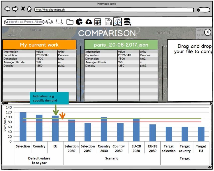
Executive Summary
Heating and cooling planning requires a consistent, robust framework about possible future pathways
of energy demand, energy carrier mix, CO2-emission factors and how developments in the electricity
and transport sector may influence the heating and cooling sector. Thus, the Hotmaps project provides
scenarios for the heating and cooling sector for EU-28 up to 2030/2050. These scenarios do not intend
to predict the future nor are they normative settings how the energy system should evolve. Rather, the
default scenarios are meant to be used by energy planners and users of the Hotmaps toolbox as starting
point for the heat planning process on local, regional or national level. The predefined scenarios, on
which the user may build to develop own, tailor made scenarios are stored in the data repository of the
Hotmaps project (https://gitlab.com/hotmaps).

The scenarios include heat demand and supply in the building and the industry sector, the electricity
generation and transport. They were developed on the country level, and partly distinguishing rural and
urban areas. In this report, we developed a methodology to break down the relevant parts of scenario
results from the country level to the local and regional level.

For the building sector (covered by the model Invert/EE-Lab ), the scenarios are mainly driven by
building renovation and construction activities and corresponding policy framework conditions,
including the installation of decentral heating and cooling systems and the uptake of district heating.
For the industry sector (covered by the model FORECAST-Industry), the scenarios comprise on the one
hand the development of macro-economic drivers, e.g. the value added or industrial production and on
the other hand energy-related indicators such as changes in the specific energy consumption due to the
diffusion of energy-efficient technologies. The whole renewable energy system with a focus on cross-
sectoral impacts, in particular biomass allocation and supply of district heating systems is covered by
the model Green-X. Overall renewable energy policies and related policy targets (and their
achievement) are main drivers of the scenarios. Scenarios for the transport sector build on the the
DIONE fleet impact model.

For each sector two scenarios with different ambition level regarding climate and energy policy targets
were developed. They are presented first by the means of fact-sheets, summarizing the characteristics
and assumptions regarding policy intensity, energy prices, technology development and key results like
energy demand or resulting share of renewable energy. These fact sheets are also available as a
documentation of Secondly, the results are discussed in a comparative way and deriving conclusions
regarding policy making and planning.

In the Hotmaps toolbox, the comparative assessment of heating and cooling planning strategies builds
on predefined indicators like energy demand by energy carriers and end-use, share of renewable energy
sources, CO2-emissions, total costs etc. The scenarios presented in this report and stored in the
Hotmaps data repository will assist energy planners in this process. The detailed process how to build
the energy planning process on pre-defined default scenarios will be described in the Hotmaps
handbook, available in spring 2019.

 4

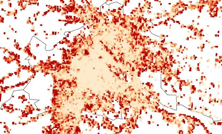
Table of Content

1 INTRODUCTION 7

2 METHODOLOGY 8
 2.1 Building related H/C demand and supply – Invert/EE-Lab 8

 2.1.1 Methodology for national scenario development 8

 2.1.2 Methodology for regional breakdown 11

 2.2 Industry related H/C demand and supply – Forecast-Industry 18

 2.2.1 Methodology for national scenario development 18

 2.2.2 Methodology for regional breakdown 20

 2.3 Electricity generation and district heating mix 22

 2.3.1 The applied modelling system: Green-X & Enertile 22

 2.3.2 General input parameter and assumptions 24

 2.4 Transport 26

 2.4.1 Methodology for national scenario development 26

 2.4.1 Methodology for regional scenario development 27

3 HEATING & COOLING SCENARIO OUTLOOK UNTIL 2050 28
 3.1 Space heating, hot water and cooling in residential and non-residential buildings 28

 3.1.1 Scenario specification 33

 3.1.2 Scenario comparison and conclusions 35

 3.2 Industry 47

 3.2.1 Scenario definition and fact sheets 47

 3.2.2 Scenario specification 51

 3.2.3 Results: Comparison of scenarios 62

 3.2.4 Conclusions 68

 3.3 Electricity generation and district heating 69

 3.3.1 Scenario definition and fact sheets 69

 3.3.2 Scenario-specific assumptions (by topical area) 75

 3.3.3 Scenario comparison and conclusions 77

 5

3.4 Transport 83

 3.4.1 Scenario description and factsheets 83

 3.4.2 Scenario comparison and conclusions 86

4 THE ROLE OF SCENARIOS IN THE HOTMAPS TOOLBOX 87

REFERENCES 89

 6

1 Introduction
Scenarios are required for heating and cooling planning and are an important means to ensure
consistency of local, regional, national and EU wide planning. Thus, the Hotmaps project provide two
scenarios for the heating and cooling sector for EU-28 up to 2030/2050. Moreover, sectors of the energy
system affecting the heating and cooling sector (transport, electricity) are also covered. Energy planners
may use these scenarios as starting point for their heat planning process on local, regional or national
level.

For this purpose, we build on models used and existing scenarios derived by the consortium in previous
projects. The scenarios include heat demand and supply in the building sector, the industry sector and
the electricity sector. Scenarios for transport have been derived from the DIONE fleet impact model.
These scenarios have been developed on the country level, and partly distinguishing rural and urban
areas. In this report, we developed a methodology to break down the relevant parts of scenario results
from the country level to the local and regional level.

The predefined scenarios, on which the user may build to develop own, tailor made scenarios also on
the local and regional level will be stored in the data repository of the Hotmaps project
(https://gitlab.com/hotmaps). Since the consortium will be also working on further scenarios during the
project duration (and probably beyond), we intend to update this scenario repository frequently.

For the building sector (covered by the model Invert/EE-Lab ), the scenarios are mainly driven by
building renovation and construction activities and corresponding policy framework conditions,
including the installation of decentral heating and cooling systems and the uptake of district heating.
For the industry sector (covered by the model FORECAST-Industry ), the scenarios comprise on the one
side the development of macro-economic drivers, e.g. the value added or industrial production and on
the other side energy-related indicators such as changes in the specific energy consumption due to the
diffusion of energy-efficient technologies. The whole renewable energy system with a focus on cross-
sectoral impacts, in particular biomass allocation and supply of district heating systems is covered by
the model Green-X. Overall renewable energy policies and related policy targets (and their
achievement) are main drivers of the scenarios. Scenarios for the transport sector build on the the
DIONE fleet impact model. DIONE is a tool for assessing key impacts of new road transport technologies
(Thiel et al., 2016).

At first, we will describe the methodology of the models and the regional breakdown of national
scenarios in chapter 2. Chapter 3 presents the scenario results by sector. Finally, we indicate the role of
scenarios in the context of the project Hotmaps and for using the Hotmaps toolbox (chapter 4).

 7

2 Methodology
In this chapter we describe the models used for the scenario development as well as the methodology
for regional breakdown. We distinguish between the following sectors: (1) Building related H/C demand
and supply – Invert/EE-Lab (chapter 2.1), (2) Industry related H/C demand and supply – Forecast-
Industry (chapter 2.2), (3) Electricity generation and district heating generation mix – Green-X (chapter
2.3) and Transport – DIONE (chapter 2.4).

 2.1 Building related H/C demand and supply – Invert/EE-
Lab
 2.1.1 Methodology for national scenario development
Invert/EE-Lab is a dynamic bottom-up building stock simulation tool. Invert/EE-Lab in particular is
designed to simulate the impact of policies and other side conditions in different scenarios (policy
scenarios, price scenarios, insulation scenarios, different consumer behaviours, etc.) and their
respective impact on future trends of energy demand and mix of renewable as well as conventional
energy sources on a national and regional level. More information is available on www.invert.at or e.g.
in Müller, (2015), Kranzl et al., (2013) or Müller, (2012). The structure and concept is described in Figure
1.

 8

Optional
 energy module
 Dynamic sub-hourly
 energy needs
 calculation

 t=t0 Energy module
 Building stock database Climate data
 Quasi-steady-state
 (t=t0, dynamic input for t1 … tn) energy balance
 approach User behavior
t=t1 … tn

 Technology databases
 Exogenously defined
 Space heating techn. Service lifetime scenario-specific
 DHW technologies module datasets
 Weibull
 Heat distr. systems distribution Growth of building stock
 Shading systems
 Ventilation systems Diffusion restrictions

 Building shell compon. Investment-decision Biomass potentials
 module Policies
 Technology combinations
 Nested logit model Options for thermal
 Database: renov. and SH-technol.
 Refurbishment techn. Logistic growth
 model Energy prices
 Preferences for heating
 Simulation results
 systems, traditions,
 • New building stock database
 inertia, ...
 • Installation of heating, refurbishment options,
 DHW systems (#, kW, m²)
 • Renovation of buildings (number, m², …)
 • Energy demand and consumption
 • CO2-emissions Data flow within simulation
 • Investments, policy program and running costs
 • … Data flow for (manual) calibration
 on an individual level

 Data flow for (manual) calibration
 on a global level

Figure 1: Overview structure of Simulation-Tool Invert/EE-Lab

The basic idea of the model is to describe the building stock, heating, cooling and hot water systems on
highly disaggregated level, calculate related energy needs and delivered energy, determine
reinvestment cycles and new investment of building components and technologies and simulate the
decisions of various agents (i.e. owner types) in case that an investment decision is due for a specific
building segment. The core of the tool is a myopical, nested logit approach, which optimizes
objectives of “agents” under imperfect information conditions and by that represents the decisions
maker concerning building related decisions.

Coverage and data structure

The model Invert/EE-Lab up to now has been applied in all countries of EU-28 (+NO, CH, IS etc.). A
representation of the implemented data of the building stock is given e.g. at www.entranze.eu.

Invert/EE-Lab covers residential and non-residential buildings. Industrial buildings are excluded (as far
as they are not included in the official statistics of office or other non-residential buildings). The level of
detail as e.g. the number of construction periods depend on the data availability and structure of
national statistics. We take into account data from Eurostat, national building statistics, national
statistics on various economic sectors for non-residential buildings, BPIE data hub, Odyssee. The current
base year used in our building stock database is 2012.

As efficiency technologies Invert/EE-Lab models the uptake of different levels of renovation measures
(country specific) and diffusion of efficient heating and hot water systems.

 9

Outputs from Invert/EE-Lab

Standard outputs from the Invert/EE-Lab on an annual basis are:
 Installation of heating, cooling and hot water systems by energy carrier and technology (number
 of buildings, number of dwellings supplied)
 Refurbishment measures by level of refurbishment (number of buildings, number of dwellings)
 Total delivered energy by energy carriers and building categories (GWh)
 Total energy need by building categories (GWh)
 Policy programme costs, e.g. support volume for investment subsidies (M€)
 Total investment (M€)
Moreover, due to the bottom-up character of the model, Invert/EE-Lab offers the possibility to derive
more detailed and other type of result evaluations as well.

Building renovation
For each building class, the Invert-EE-Lab model considers up to 9 different renovation bundles, which
consists of refurbishment options for different building components such as windows, upper ceiling,
exterior walls, floor, shading systems, space heating distribution system and others at different levels
of energy saving ambitious and associated investment needs. Usually, we use define three different
renovation options (renovation bundle) per building, which are standard renovation and two intensified
renovation options, as well as a maintenance option without any improvement of the building envelope.

Specific heating energy-uses covered
In the Invert/EE-Lab model, the following building related energy usage types and energy carriers are
covered:

 Space heating: oil, gas and coal powered heating systems, biomass heating systems, electricity
 convectors, heat pumps and solar thermal collectors
 Domestic hot water: oil and gas systems, biomass powered water heating, electrical converters,
 heat pumps and solar thermal collectors
 Auxiliary energy: technology related auxiliary energy demand of heating systems
 Cooling: energy demand for cooling

Scenario-independent drivers
The energy demand of buildings and for the usage types mentioned above depends on a variety of
exogenous drivers, which are the same for all scenarios. These drivers include, number of
buildings/dwellings, floor area, climate development, solar yield, fuel prices.

Modelling of policy instruments
The model Invert/EE-Lab allows for a wide range of policies to be defined for each country. For existing
policies a major data source for defining the inputs for the model is the MURE database which includes
descriptions of polices measures such as:

 Minimum energy performance standards (MEPS) set by the Ecodesign directive

 10

Minimum energy performance standards for major refurbishments and newly constructed
 buildings, including the definition of Nearly Zero Energy Buildings (NZEBs) defined in the
 national implementations of the Directive on Energy Performance of buildings.
 Energy taxes for different energy carriers
 Investment subsidies, grants, soft loans (considering constrains regarding the absolute support
 level either per building or dwelling as well as restricted national budgets per country and
 support instrument) for different types of refurbish measures and building types as well as
 investments into technologies to utilize renewable energy carriers.
 “Soft measures” such as reducing the information barrier and increasing the compliance rate
 through the introduction of energy performance certificates, information campaigns, or
 reducing the diffusion barrier through workforce education, etc.

The policy descriptions lead to the following implementation in the simulation:
 Investment subsidies for building renovation (three options for building envelope
 refurbishment)
 Investment subsidies for heating supply systems
 Investment subsidies for solar thermal systems
 Country specific public budgets for subsidies
 Obligations regarding the implantation of renewable heating supply systems
 Building codes: improvement of technical building standards for new and renovated buildings
 (building envelope),

 2.1.2 Methodology for regional breakdown
The trajectories derived by the Invert/EE-Lab model represent the developments in the sector at an
aggregated regional level. For the current implementation of the building stock, this means the NUTS 0
level (countries) for the very most countries. In order to break down the scenarios to regional and local
level, the national development needs to be transferred consistently to the regional building stock.

This breakdown is done by a two-step approach. In the first step, we derive consistent scenarios for the
useful energy demand on the NUTS 3 level. In the second step, the development on the NUTS 3 level is
transferred to the local level of the heat density maps. For the interpretation of the results it is important
to bear in mind that this break-down is done based on a generic approach and generic data and that the
local circumstances cannot fully be taken into account. However, the applied algorithm ensures that the
results on the local level will consistently sum up to national development for each scenario.

Transfer of NUTS 0 scenario results to the NUTS 3 level

At the NUTS 3 level, the following indicators, which specify the energy needs (useful energy demand)
are available:

For residential buildings:

 11

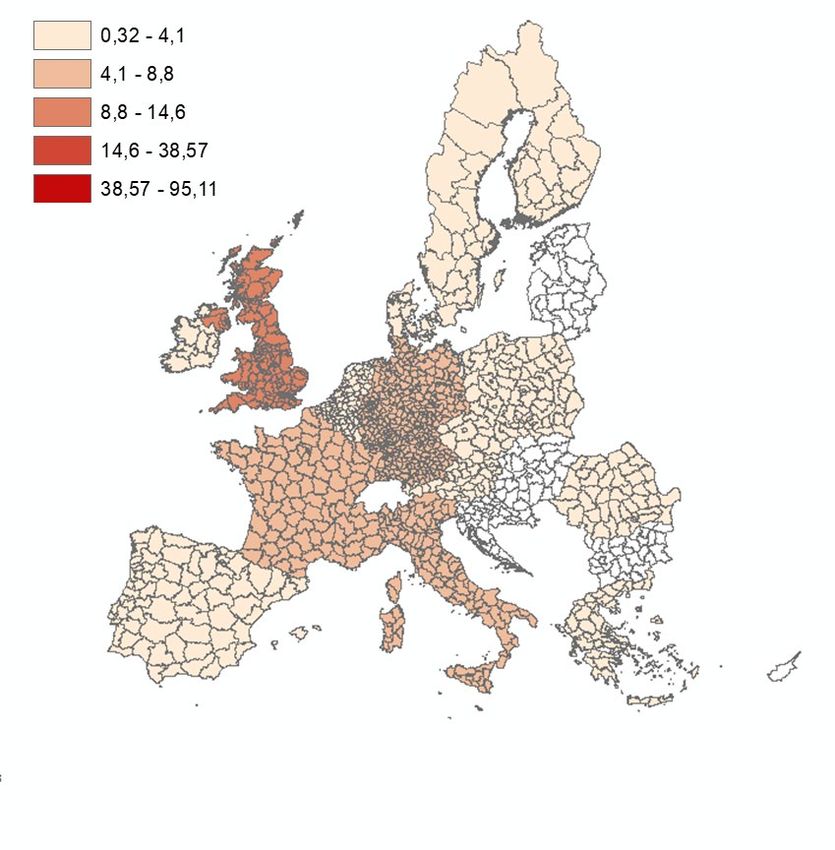
Data provided by the European Census Hub 2011 (Census 2011, Population and Housing Census
 2011):
 o Useful floor area per dwelling
 o Population
 o Number of dwellings
 o Number of dwellings per building type
 o Number of dwellings per construction period
 Heating and cooling-degree days (HDD and CDD) on NUTS2-level based on Eurostat (Eurostat, 2013).
 Within the NUTS2 level, the HDD and CDD on the NUTS3 level are calculated based on the average
 HDD (18.5/18.5) and CDD (22.5/22.5) calculated from the observed daily temperatures on a 25 x 25
 km grid for the period 2002-2012 (see (Haylock, M.R. et al., 2011)).
For non-residential buildings:
 Population, heating degree days (HDD) and cooling degree days (CDD), the final energy
 consumption(FEC) per m² floor area and building type based on the Invert/EE-Lab building stock
 database (Eurostat, 2011)
 The estimated share per construction periods based on the distribution of the construction periods
 of apartment buildings (Eurostat, 2011)
 The total value added of the service sector (Eurostat, 2016)
 The sectoral value added (VA): (a) Accommodation, restaurants, stores and warehouses, (b) other
 private services and (c) public buildings, research and education, art, culture and health sector
 (Eurostat, 2016).
Furthermore, on the NUTS0 level we use data such as the final energy consumption per m² floor area
and building type based on Invert/EE-Lab model results. These data have been derived within the
European project “Mapping_HC: Mapping and analysis of the current and future (2020-2030)
heating/cooling fuel deployment (fossil and renewables)” (EC service contract ENER/C2/2014-
641/SI2.697512) (Fleiter, Tobias et al., 2016) as well as scenarios for the development until 2050 from
the H2020 project SetNav 1, which are currently under development.
In a first step, we estimate the development of the population growth for each NUTS 3 region2. This is
done by putting the historic population growth (2002 – 2017, (Eurostat, 2018)) of each NUTS3 region
(using an exponentially distributed weighting factor with a decline rate 0.25) in relation to the national
population growth. The relative growth of a given NUTS3 region ∆ , 3 is calculated by using growth
rate of the given NUTS3 region between 2002 and 2017 3,2002,2017 minus the national growth
rate 0,2002,2017 for the same period:

 ∆ , 3 = 3,2002,2017 − 0,2002,2017

1
 http://www.set-nav.eu/
2
 Until March 2017, the projected change of the population by NUTS3 regions was available at Eurostat (Code:
proj_13rpms3). Unfortunately, the data have been removed and only a map of the results exists anymore (see
http://ec.europa.eu/eurostat/statistics-
explained/images/f/f8/Projected_percentage_change_of_the_population%2C_by_NUTS_3_regions%2C_2015%E
2%80%9350_%28%C2%B9%29_%28%25%29_RYB2016.png)

 12

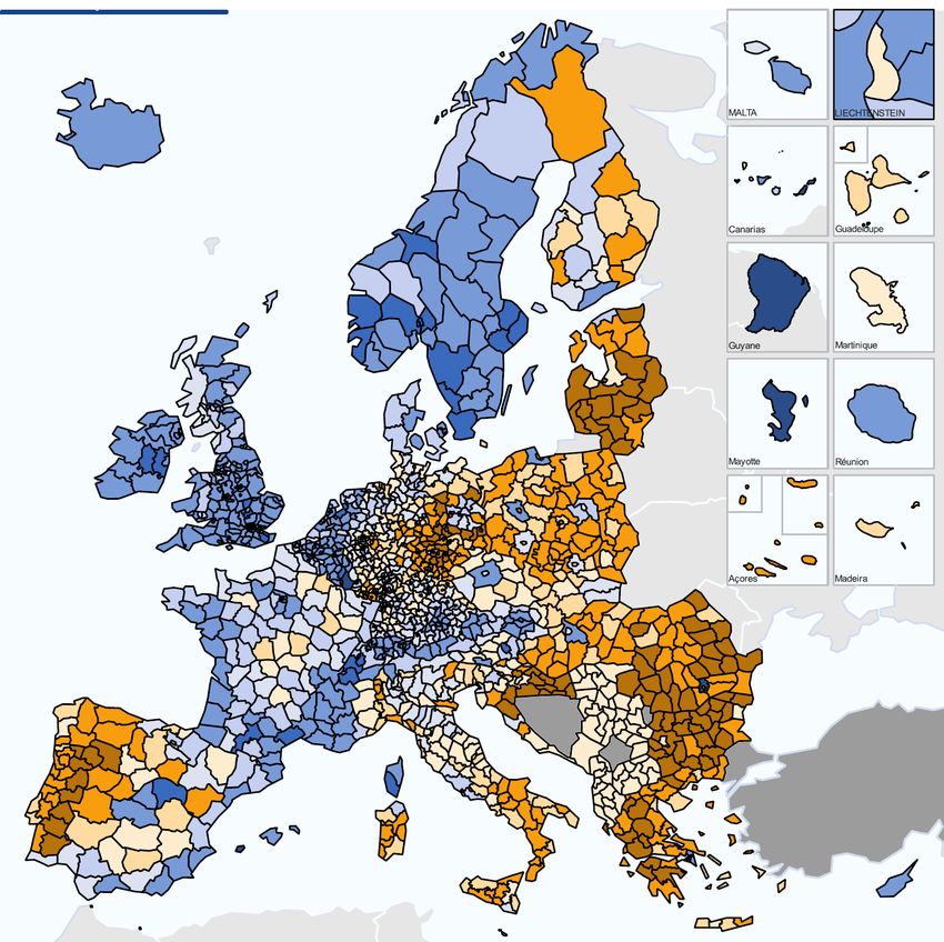
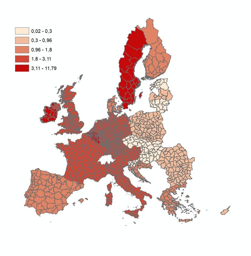
−0.05 ≤ ∆ , 3 ≤ +0.08

The future annual growth rate of a given NUTS3 region in a given year t+1 3, , +1 is then calculated
by adding the relative growth multiplied by a weighting factor to the national growth rate in that
given year and multiplied by a correction term. For the weighting factor, we assume it is 0.8 in 2018,
declines linearly to 0.5 within a 10-year period and remains afterwards at this level.
 3, , +1, = � 0, , +1 + ∙ ∆ , 3 � ∙ min� 3, , 3,2002 �

 3, +1, = 3, ∙ 3, , +1, 

 3
 ∆ , 0, +1 = 0, +1 − � 3, +1, 
 1

 = ∆ , 0, +1
 3 | � 3, , +1, � = � 0, , +1�
 / �� 3, +1, 
 1
 3 | � 3, , +1, � ≠ � 0, , +1 �
 +2� 3, +1, �
 1

The population is then calculated by
 3, +1, ∗ (1 + ) � 3 | � , , +1, � = � 0, , +1 ��
 3, +1 = � �
 3, +1, ∗ (1 − 2 ∗ ) � 3 | � , , +1, � ≠ � 0, , +1 ��

For the national population growth, we draw on forecast data published by Eurostat (Baseline
projections, proj_15npms 3). Based on this approach we get annual growth rates of the different
European NUTS 3 regions in the range of – 1.3 %p.a. to about +1 %p.a. (Figure 2). The change of the
population between 2015 and 2050 per region is depicted in Figure 3.

 Annual growth rate of NUTS 3 regions
 2.5%

 2.0%
 Annual growth rate 2017 - 2050

 1.5%

 1.0%

 0.5%

 0.0%

 -0.5%

 -1.0%

 -1.5%
 -1.5% -1.0% -0.5% 0.0% 0.5% 1.0% 1.5% 2.0% 2.5%
 Annual growth rate 2002 - 2017

Figure 2: Future annual growth rate (2015 – 2050) versus historical growth rate (2002 – 2012) for the European NUTS 3
regions.

3
 Population on 1st January by age, sex and type of projection, Code: proj_15npms, Last update of data:
19/06/2017

 13

Figure 3: Estimated change of the population by NUTS3 regions, 2015 – 2050.

The heated net floor area of residential buildings is then derived by the net floor area per capita and the
population of that region. For regions with currently low value added per capita (below 20 tds. Euros
per capita and year), we consider an additional living space demand per capita in the future. For regions
with a higher added value per capita in 2012 we assume a constant residential floor space per capita in
the future (see Figure 44). For the development of the non-residential sector, we assume that the
heated gross floor area increases (or decreases) with the population growth.

 14

Figure 4: Correlation of economic activities and average net floor area per capita (base year 2012). (Source: Schremmer et al.,
2017)

In a second step, we determine the building demolition rate per construction period and building type
(small residential buildings: residential buildings with up to two apartments per building and
row/terrace houses; medium and large residential building and non-residential buildings). Since
statistical data on the construction period of non-residential buildings are currently not available, we
assume that these building types have the same age distribution as medium and large residential
buildings. We than apply the national demolition rate per building type and construction period (four
different historical construction periods) on the NUTS 3 level.

The difference between the remaining floor area of existing buildings and the total demand derived in
the first step based on the population constitutes the demand for newly constructed buildings. For
most countries, the national annual demolition rates are currently in the range of about 0.3 – 0.5 %p.a.,
whereas the construction rate lies in the order of about 0.7 – 1.5 % p.a. If the population declines with
a higher rate than the demolition rate, this leads to the situation that the existing buildings stock would
fulfil the required demand for living space and the construction rate would subsequently drop to zero.
To prevent this outcome, we add the condition that demolition rate needs to exceed the population
decline rate of at least 0.2 %p.a., which gives a lower boundary for the annual construction rate of 0.2
%.

In a third step, the refurbishment rate of the existing building stock on the NUTS3 level is calculated
from the national results. This step again draws on the national refurbishment rates per building type
and construction period and transfer the development derived on the NUTS0 level to the NUTS3 level.
For the refurbishment rate, we don’t consider a lower bound as we do for the construction rate. Instead,
we assume that the thermal renovation rate scales with the heating cost. We use the heating degree-
days as indicator for the distribution of heating costs within each country. The total annual energy costs
for heating derive from the energy consumption for space heating and domestic hot water production.
If we leave the impact of different heating systems and energy carriers aside, then the energy costs

 15

follow the heating degree days (very roughly) with an elasticity of about 0.7 4. Based on this correlation
we calculate the refurbishment rate at the NUTS3 level , 3 (for a given building type and
construction period and the current policy scenario where no enforced building renovation policies are
in force) based on:

 50% ∙0.7
 , 3 = , 0 ∙ � 3 � ∙ ,
 0

where denotes for the heating degree days, , 0 is the refurbishment rate at the national
level and is a correction factor to ensure that the sum of the regional refurbishment activities is
consistent with the national results.

The energy needs for space heating, domestic hot water preparation and air conditioning at the NUTS3
level is then derived by the energy needs of the remaining existing buildings stock corrected by the
effects of thermal building renovation
(1- , 3 ) ∙ ( / ) plus the energy needs of the newly
constructed buildings.

Transfer of NUTS 3 results to the spatial heat density map on 100*100 m level

For the spatial distributed building stock properties of the local building stock we can only draw on
estimates of the population, covered plot area (for different periods) as well as the openstreetmap
project database, which however doesn’t cover all areas and all buildings. Furthermore, the historic
development of the population below the NUTS3 level is not available or uncertain for a larger share of
regions, especially since the borders of the local administrative units (LAU) changed considerable within
the last 2 decades in many countries. Therefore, we have to make additional presumptions and
simplifications regarding the local development.

A first presumption is that the population growth rate of a given LAU region compared to the
development of the whole NUTS3 region depends on the population density on areas (hectare) with a
sealed soil of the LAU region (densPOPLAU) compared to this indicator of the NUTS3 region
(densPOPNUTS3).

 , , +1 = 3, , +1 ∙ � � ∙ 
 3

The factor ensures again that the sum of the local development amounts to the overall
development, the elasticity defines the strength of this individual population growth. If is set to zero
then all areas within a NUTS3 regions have the same growth rate, it > 0, then population growth is
higher in densely populated areas, which leads to an additional densification of the population,
reflecting the phenomenon of increasing urbanisation.

The second presumption is that the building demolition rate (per construction period, see Figure 5) is
uniformly distributed within a NUTS3 region. For the refurbishment rate, we apply the same approach

4
 Based on the energy demand for space heating and domestic hot water preparation. In colder regions, the
elasticity is higher, in warmer regions (still continental Europe) the elasticity is in the range of 0.4 to 0.5.
Furthermore, the elasticity is lower for more energy efficient buildings than it is for buildings with higher area
specific space heat demand.

 16

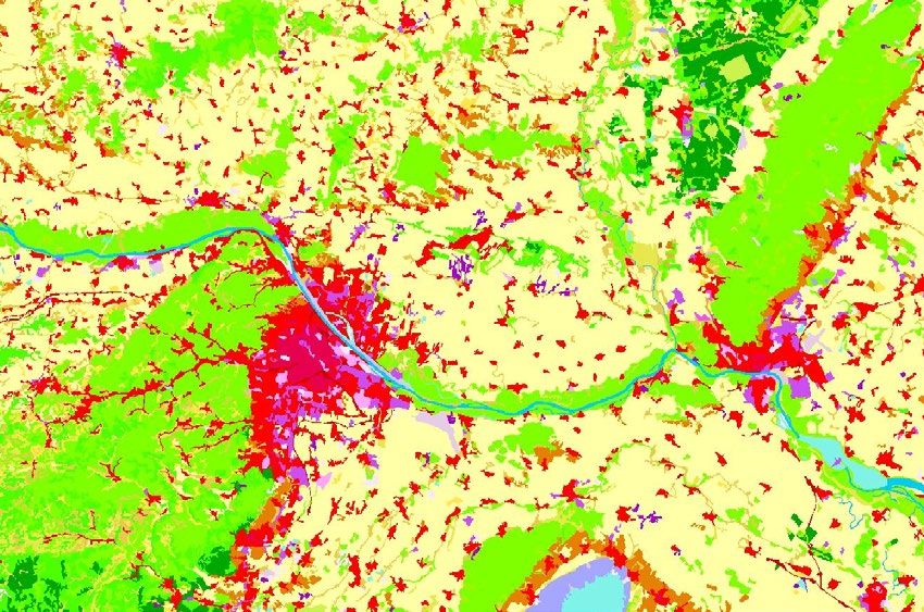
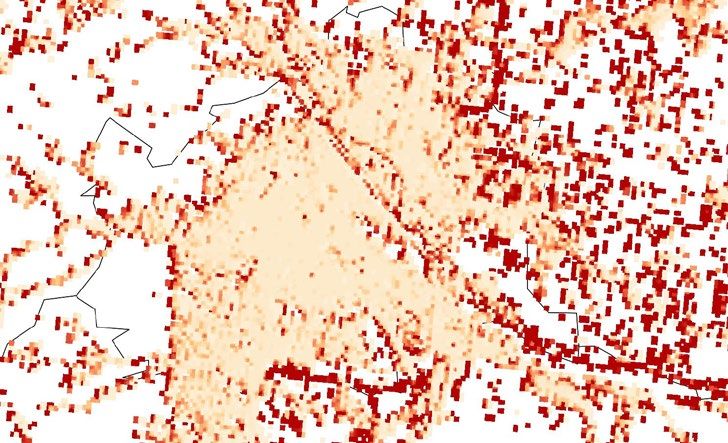
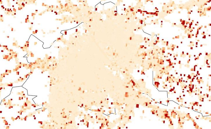
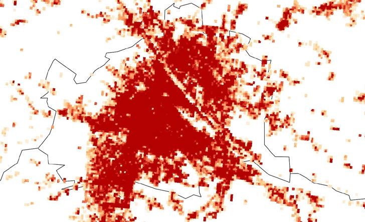
as used by the breakdown of the national results to the NUTS3 level. On a very local level this leads to
the paradox situation that individual buildings will be only partly torn down or refurbished. This should
be interpreted as probability distribution that buildings will be demolished or refurbished in a certain
area.

 before 1975 1975-1990

 1990-2000 2000-2014

Figure 5. Estimated share of buildings per construction period for the region of Vienna. High shares (+75 %) are color-coded in
red, low shares (

be constructed virtually on every suitable land plot. Therefore, rules how to distribute the new buildings
need to be defined in our approach. In this project, we apply the following approach:

 1. New buildings replace existing buildings, which were torn down according to the demolition
 rate.
 2. The remaining share will be distributed between hectare cells on which buildings are already
 constructed (using the indicators: existing plot ratio and recent construction activities (past 15
 years)), as well as hectare cells which, which have a low soil sealing and could be settled from
 its land cover type.

In the process of breaking down scenario data until 2030 and 2050 from NUTS3 to hectare level, we will
define the share to which we will distribute newly constructed building among those possibilities, also
taking into account calibration through Hotmaps pilot areas. By putting too much weight on the current
plot ratio, the results will lead to an overestimation of the future heat densities and thus the suitability
of district heating. The recent construction activities appear to be a plausible indicator for a few years.
However, it’s validity in the long run is not as obvious. From this point of view, we favour to set a higher
weight on areas which are not settled or only partly settled but appear to be suitable for settlements
based on Corine land cover data (Discontinuous urban fabric, Complex cultivation pattern) and are
located next to current construction activities for the more distant future.

Figure 7. Corine land cover data on the information of land usage type on the hectare level. (Source: European Environment
Agency (EEA), 2012)

The calculation of the energy needs for space heating and domestic hot water preparation will follow
the same approach as described in the section above.

 2.2 Industry related H/C demand and supply – Forecast-
Industry
 2.2.1 Methodology for national scenario development
The FORECAST modelling platform aims to develop long-term scenarios for future energy demand of
individual countries and world regions until 2050. It is based on a bottom-up modelling approach
considering the dynamics of technologies and socio-economic drivers. The model allows addressing

 18

various research questions related to energy demand including scenarios for the future demand of
individual energy carriers like electricity or natural gas, calculating energy saving potentials and the
impact on greenhouse gas (GHG) emissions as well as abatement cost curves and ex-ante policy impact
assessments.

FORECAST is a simulation model used to support investment decisions, taking into consideration
barriers to the adoption of energy efficient technologies as well as various policy instruments such as
standards, taxes and subsidies. Different approaches are used to simulate technology diffusion,
including diffusion curves, vintage stock models and discrete choice simulation.

Figure 8 shows the simplified structure of FORECAST-Industry. Main macro-economic drivers are
industrial production for over 70 individually modelled basic materials products, gross value added for
less energy-intensive sub-sectors and the employment numbers. Five sub-modules cover: basic
materials processes, space heating, electric motor systems, furnaces and steam systems.
 Macro
 Input dat a Result s
 Material ef f iciency Circular economy Structural change
 Drivers Energy demand
 - GDP Drivers: Production, value added, employment, end-user energy prices - Final energy
 - Population - Delivered energy
 - Energy prices - Usef ul energy
 - Temperature
 - Business cycle Energy-intensive Space heating &
 Processes cooling GHG emissions
 - Energy-related
 Policy
 - EU ETS
 - Taxes Process energy Buildings stock
 - Process related

 Bottom-up
 - CO2-price demand Calibration model
 - Standards End-use energy
 - Grants Saving option Heating systems
 balance Costs
 - OPEX support dif f usion stock model
 - Investment
 - Policy cost
 Structure - Energy spending
 - Energy balance Electric motors Furnaces Steam & hot w ater
 - Emissions & lighting
 balance Indicators
 Saving options System ef f iciency
 - Technology Fuel sw itch - Levelised costs
 Cross-cutting
 dif f usion
 distribution of process heat
 Steam generation
 stock model - Energy savings
 Technology & - Technology and
 Behaviour f uel mix
 - Ef f iciency Results by sub-sector, energy carrier, temp. level, end-use, country - SEC by process
 - Savings - Technology
 - CAPEX, OPEX Market shares
 - Learning - CHP generation
 Interfaces and add-ons
 - Emissions - Frozen ef f iciency
 - Lif etime Load curves and Regional diss- - Heat and cold
 CCS dif f usion Excess heat temperatures
 - Pref erences demand response aggregation

 Source: FORECAST

Figure 8: Overview of the bottom-up model FORECAST-Industry

For this study, the three sub-modules related to the CO2-intensive industries are of high importance:

 1. Energy-intensive processes: This module covers 76 individual processes/products via their
 (physical) production output and specific energy consumption (SEC). The diffusion of about 200
 individual saving options is modelled based on their payback period (Fleiter et al. 2013; Fleiter
 et al. 2012). Saving options can represent energy efficiency improvements, but also internal use
 of excess heat, material efficiency or savings of process-related emissions.
 2. Space heating and cooling: Space heating accounts for about 9% of final energy demand in the
 German industry. We use a vintage stock model for buildings and space heating technologies.

 19

The model distinguishes between offices and production facilities for individual sub-sectors. It
 considers the construction, refurbishment and demolition of buildings as well as the
 construction and dismantling of space heating technologies. Investment in space heating
 technologies such as natural gas boilers or heat pumps is determined based on a discrete choice
 approach (Biere 2015).
 3. Electric motors and lighting: These cross-cutting technologies (CCTs) include pumps, ventilation
 systems, compressed air systems, machine tools, cold appliances, other motor appliances and
 lighting. The module captures individual units as well as the entire motor-driven system,
 including losses in transmission between conversion units. The diffusion of saving options is
 modelled in a similar way to the approach used for process-specific saving options.
 4. Furnaces: energy demand in furnaces uses the bottom-up estimations from the module
 “energy-intensive processes”. Furnaces are found across most industrial sub-sectors and are
 very specific to the production process. Typically, they require very high temperature heat. The
 furnaces module simulates price-based fuel switching using a random utility model (for more
 details, see (Rehfeldt et al. 2018)).
 5. Steam and hot water: the remaining process heat (

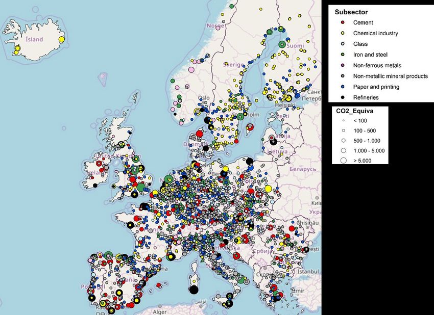
databases, only energy intensive industries like steel, paper, glass, cement and chemicals industries. The
distribution of sectors and emission across Europe is illustrated in Figure 9.

FORECAST Industry uses the national physical production in tonnes per year as a main driver for energy
demand. As a distribution key to the individual sites, the physical production per process is a good
indicator for site-specific energy demand. This implies that the process and the annual production of all
industrial sites should be included in the database. As mentioned above, this is possible for energy
intensive industrial sub-sectors, but not for all. Even for these sectors, some smaller plants could be
missing.

Figure 9: Industrial sites in the industrial database differentiated by subsector and emissions

The methodology for the breakdown of national industrial energy demand to the NUTS3 regions will
therefore be different for the industrial sub-sectors, following two alternative methods, see Figure 10.
First, for sub-sectors for which the physical production is known for almost all plants, the heating and
cooling demand can be distributed based on the production data in the base year. In the time horizon
until 2050 it should be stated that there are uncertainties about closure or opening of individual sites.
As only the development of the production is projected based on the economic development,
information about individual sites is lacking naturally. As it is impossible to predict these individual
decisions of companies, it is decided to distribute the national development equally across the industrial
sites of each sector. For example, if the cement industry has an increasing physical output until 2050,
the individual sites have the same relative increase instead of opening another facility. Another case
would be the change of a process or fuel switch. For decarbonisation of industry, a higher share of
electric arc furnaces is needed. This change will happen as a binary decision. If a blast furnace reaches
a certain age, it could be possible to switch to an electric arc furnace. This includes another dimension
of distribution keys, as not only the physical production, but also the age of certain facilities plays a

 21

major role. For the steel sector, a stock model is applied in FORECAST industry, which can be also
georeferenced by the database, as the age of the facilities is included from the sectoral database.

 Data Input Regionalization Output

 Sectoral value added, Industrial energy
Top-down

 All other subsectors
 number of employees demand NUTS 3

 • Machinery • Depending on data
 • Food availability
 • Others

 Site-specific final Site-specific energy
 Industrial Sites
 energy consumption demand
Bottom-up

 • Iron and Steel • 40 different processes • Energy and material
 • Non-metallic minerals • Defined in industrial efficiency equally
 • Chemicals sites database distributed
 • Pulp and paper • Probability of fuel switch

Figure 10: Methodology for regionalization of the energy demand, differentiated by industrial subsectors

Second, for sub-sectors, where no sectoral database is available, or it is not complete in terms of
production capacity or age of facilities, the mentioned uncertainties can be much higher. Furthermore,
it is not possible to distribute the energy demand of heterogeneous sectors to single industrial sites,
where not all sites are included in the database. The reason for this could be that they do not emit
greenhouse gases above the threshold value to be listed in the database, e.g. in the sectors machinery
or food and tobacco. For these sectors another methodology needs to be chosen. The sectoral gross
value added in the resolution of NUTS 3 level provides a suitable indicator for distributing the national
energy demand. If that is not available for all countries, other indicators need to be chosen, e.g. number
of employees or population density. Therefore, the industrial heating and cooling demand for those
sectors is not available site-specific, only on a resolution of NUTS 3 regions.

 2.3 Electricity generation and district heating mix
 2.3.1 The applied modelling system: Green-X & Enertile
This analysis builds on modelling works undertaken by the use of TU Wien’s Green-X model (cf. Box 1),
closely linked to Fraunhofer ISI’s Enertile model (cf. Box 2). More precisely, Green-X delivers a first
picture of future RES developments under distinct energy policy trends, indicating details on technology
trends (investments, installed capacities and generation) and the geographical distribution of RES
deployment as well as related costs (generation cost), expenditures (capital, operation and support
expenditures) and benefits (avoided fossil fuels and related carbon emissions). For assessing the
interplay between RES and the future electricity market, Green-X was complemented by its power-
system companion, i.e. the Enertile model. Thanks to a higher intertemporal resolution than in the RES
investment model Green-X, Enertile enables a deeper analysis of the merit order effect and related

 22

market values of the produced electricity of variable and dispatchable renewables and, therefore, can
shed further light on the interplay between supply, demand and storage in the electricity sector.
Box 1: Brief characterization of the Green-X model

 Green-X is an energy system model that offers a detailed representation of RES potentials and
 related technologies in Europe and in neighbouring countries. It aims at indicating consequences of
 RES policy choices in a real-world energy policy context thanks to its comprehensive incorporation of
 various energy policy instruments including related design features. The model simulates technology-
 specific RES deployment by country on a yearly basis, in the time span up to 2050, taking into account
 the impact of dedicated support schemes as well as economic and non-economic framework
 conditions (e.g. regulatory and societal constraints). Moreover, the model allows for an appropriate
 representation of financing conditions and of the related impact on investor’s risk. This, in turn, allows
 conducting in-depth analyses of future RES deployment and corresponding costs, expenditures and
 benefits arising from the preconditioned policy choices on country, sector and technology level.
Box 2: Brief characterization of the Enertile model

 Enertile is an energy system optimization model developed at the Fraunhofer Institute for System and
 Innovation Research ISI. The model focuses on the power sector, but also covers the interdependencies
 with other sectors, especially heating &cooling and the transport sector. It is used mostly for long-
 term scenario studies and is explicitly designed to depict the challenges and opportunities of
 increasing shares of renewable energies.
 A major advantage of the model is its high technical and temporal resolution – i.e. the model
 features a full hourly resolution: In each analysed year, 8,760 hours are covered. Since real weather
 data is applied, the interdependencies between weather regions and renewable technologies are
 implicitly included.
 Moreover, Enertile allows for a full optimization of the investments into all major infrastructures of
 the power sector 6, including conventional power generation, combined-heat-and-power (CHP),
 renewable power technologies, cross-border transmission grids, and flexibility options such as
 demand-side-management (DSM) and power-to-heat storage technologies. The model chooses the
 optimal portfolio of technologies while determining the utilization of these for all hours of each
 analysed year.

6For the purpose of this assessment, investments in RES technologies were taken from Green-X modelling. Thus,
Enertile focussed on modelling complementary investment needs as well as power plant dispatch.

 23

Electricity system
 model, power
 plant dispatch Electricity prices,
 Market values,

 Case Study Analysis
 Optimal RES-E share,
 Curtailment

 costs and benefits
 Enertile Green-X

 RES-E installed
 capacities and cost
 (investment, operation) RES investment model,
 detailed energy policy
 representation

 Figure 11: Model coupling between Enertile (left) and Green-X (right) for a detailed assessment of RES developments in the
 electricity sector

Figure 11 gives an overview on the interplay of both models. Both models are operated with the same
set of general input parameters, however in different spatial and temporal resolution. Green-X delivers
a first picture of renewables deployment and related costs, expenditures and benefits by country on a
yearly basis (2010 to 2050). The output of Green-X in terms of country- and technology-specific RES
capacities and generation in the electricity sector for selected years (2020, 2030 and 2050) serves as
input for the power-system analysis done with Enertile. Subsequently, the Enertile model analyses the
interplay between supply, demand, and storage in the electricity sector on an hourly basis for the given
years. The output of Enertile is then fed back into the RES investment model Green-X. In particular, the
feedback comprises the amount of RES that can be integrated into the grids, the electricity prices, and
corresponding market revenues (i.e. market values of the electricity produced by variable and
dispatchable RES-E) of all assessed RES-E technologies for each assessed country.

 2.3.2 General input parameter and assumptions
In order to ensure maximum consistency with existing EU scenarios and projections the key input
parameters of the scenarios presented in this report are derived from PRIMES modelling and from the
Green-X database (www.green-x.at) with respect to the potentials and cost of RES technologies. As
indicated in Table 13 (above), PRIMES comes into play for energy demand developments as well as
fossil energy and carbon price trends. The specific PRIMES scenarios used are the latest publicly
available reference scenario (European Commission, 2016f) and the climate mitigation scenarios
PRIMES euco27 and PRIMES euco30 that build on the targeted use of renewables (i.e. 27% RES by 2030)
and an enhanced use of energy efficiency (EE) compared to reference conditions – i.e. 27% (euco27) or
30% EE (euco30) by 2030, respectively. Please note that all PRIMES scenarios are intensively discussed
in the EC’s winter package, cf. the Impact assessment of the recast RED (SWD (2016) 410 final)
(European Commission, 2016).

With respect to the underlying policy concept and ambition level for RES and energy efficiency, the
following assumptions are taken for the assessed scenarios:

 A common policy framework until 2020: All scenarios build on common ground for the near
 future, i.e. the years up to 2020. Here, a strengthening of national RES policies is presumed,
 serving to meet the given 2020 RES targets. Each country uses national (in most cases

 24

technology-specific) support schemes in the electricity sector to meet its own 2020 RES target,
 complemented by RES cooperation between Member States in the case of insufficient or
 comparatively expensive domestic renewable sources. Please note that support levels are
 tailored to the national needs, in other words, they are generally based on the technology
 specific generation costs at country level.
 A “least-cost” approach for RES post 2020: For renewables, the default ambition level is set
 at 27% - i.e. achieving a RES share in gross final energy demand in size of at least 27% by 2030
 and beyond.7 Conceptually, the scenarios follow a simplified policy concept for renewables: The
 underlying policy concept for incentivising RES can be characterised as a “least-cost” approach,
 enhancing an efficient use of RES for meeting the 2030 EU RES target in a cost-effective manner
 as outlined in Box 3.
 Please note that this “virtual” policy concept matches perfectly with the objective of this
 case study. Thus, the RES policy approach taken in modelling allows for deriving the optimal
 RES-E or RES-H share under given assumptions from a European least (policy) cost perspective
 – i.e. allowing for minimising support expenditures required for meeting a certain overall RES
 target by 2030 and beyond. Thus, the undertaken least cost allocation of the RES efforts to the
 available RES technologies across all energy sectors (electricity, heat, transport fuels) and
 countries (EU28 Member States) delivers an optimal RES deployment under given constraints.
 Concerning the role of energy efficiency, a moderate ambition level is presumed – i.e. in
 accordance with the PRIMES euco27 scenario, gross final energy demand is reduced by 27% in
 2030 compared to baseline conditions.

Box 3: A least-cost approach to allocate investments in RES technologies post 2020

 The selection of RES technologies in the period post 2020 in all assessed cases within this exercise
 follows a least-cost approach, meaning that all additionally required future RES technology options
 are ranked in a merit-order, and it is left to the economic viability which options are chosen for
 meeting the presumed 2030 RES target. In other words, a least-cost approach is used to determine
 investments in RES technologies post 2020 across the EU. This allows for a full reflection of
 competition across technologies and countries (incorporating well also differences in financing
 conditions etc.) from a European perspective. Support levels and related expenditures follow then the
 marginal pricing concept where the marginal technology option determines the support level (like in
 the ETS or in a quota/certificate trading regime, or similar to the concept of liberalised electricity
 markets).

7
 The overall RES target as presumed for 2030 – i.e. as default (at least) 27% RES share in gross final energy
demand – is maintained in modelling as minimum target also for the period post 2030 (until 2050). Draft results
show, however, that in all assessed scenarios the minimum target level is over fulfilled, meaning that RES
deployment is then well above 27% in the years up to 2050.

 25

2.4 Transport
 2.4.1 Methodology for national scenario development
To simulate energy demand from the transport sector in 2050, the DIONE fleet impact model was used.
DIONE is a tool for assessing key impacts of new road transport technologies (Thiel et al., 2016). The
model consists of five modules: Stock, Cost, Mileage, Energy Consumption and Emission (for technical
details about the model, see (EMISIA, 2014)).
Table 1: Vehicle categories, by powertrain

 Powertrains PC LCV HDV Bus
 Gasoline X X X
 Diesel X X X X
 FFV X X
 LPG X
 CNG X X
 HEV X
 PHEV / EREV X
 BEV X
 FCV X 8

Legend: X indicates that this option is available in DIONE. Source: DIONE model

Four vehicle categories are included in DIONE: passenger cars (PCs), light commercial vehicles (LCVs),
heavy-duty vehicles (HDVs), buses and two-wheelers. The latter is not included in this study. Table 1
shows powertrain availability in DIONE, for each vehicle category.
Table 2: Passenger car sizes, by engine capacity

 Tiny Small Medium Large
 < 0.8 l < 1.4 l* 1.4 l – 2.0 l > 2.0 l
*Except for gasoline, which is defined as 0.8 l – 1.4 l because this powertrain also has the size ‘tiny’.

The calibrated base year in DIONE is 2010. For historical data, the model relies on TRACCS but adopts a
classification based on engine capacity (for PCs, see Table 2). Electricity consumption factors were
derived from real drive data from the Green eMotion project. For the future, DIONE follows the trends
of PRIMES-TREMOVE 2012 (baseline scenario with adopted measures). DIONE can be used to construct
scenarios until 2050, using an annual resolution. Table 3 shows powertrain availability by car size

8
 FFV: Flexible-fuel vehicle; LPG: liquefied petroleum CNG: Compressed natural gas vehicles; HEV: hybrid electric
vehicle; PHEV/EREv: plug-in hybrid electric vehicle/extended-range electric vehicle; BEV: battery electric vehicle;
FCV: fuel cell vehicle

 26

Table 3: Passenger car sizes, by powertrain

 Powertrains Tiny Small Medium Large
 Gasoline X* X X X
 Diesel X* X X
 FFV X
 LPG X X X
 CNG X X X
 HEV X X
 PHEV / EREV X
 BEV X
 FCV X
*Included in DIONE, but set to zero in the baseline scenario. Source: DIONE model

 2.4.1 Methodology for regional scenario development
The historical data points are extrapolated based on future trends for selected indicators: vehicle stock
(NUTS1), energy demand (NUTS1), GDP/capita (NUTS3), population density (NUTS3) derived from the
PRIMES –TREMOVE EU 2016 reference scenario and DIONE model. The geographical datasets on
boundaries of NUTS 3 regions was obtained from the GISCO database (GISCO, 2018). Each of parameters
was afterwards inserted in the GIS database using ArcGIS 10.4© software in layers as polygons, out of
which the grids with a 8000 × 8000 m size of raster cell is created.

 27

3 Heating & Cooling scenario outlook until
2050
In this chapter we describe the model based scenario results on country level for the building sector
(chapter 3.1), the industry sector (chapter 3.2), district heating and electricity generation (chapter 3.3)
and transport (chapter 3.4).

We will apply the structure of a factsheet for outlining and communicating the key characteristics,
assumptions as well as input and output data of the scenarios. These fact sheets will also be uploaded
as meta-data description in the GitLab data repository. The user of the toolbox will be able to download
more detailed country and region specific data from the toolbox. Moreover, it is planned to upload
additional scenarios later in in the project in the Hotmaps data repository
(https://gitlab.com/hotmaps/). More details (beyond these two pages) should be provided as additional
text in this report. However, only the fact sheet information will be uploaded in GitLab for the scenario
characterisation.

 3.1 Space heating, hot water and cooling in residential and
non-residential buildings
This chapter presents scenario data for space heating, hot water and cooling in residential and non-
residential buildings on country level for EU-28 until 2050. We show two scenarios: (1) A current policy
scenario, assuming that currently existing policies remain in place and (2) a more ambitious policy
scenario with moderately enhanced climate mitigation policies. However, also the second scenario is
not a really strong decarbonisation scenario in line with Paris COP 21 targets. Stronger decarbonisation
scenarios will be added later during the project duration to the Hotmaps data repository.

Both scenarios on the country level are based on scenarios developed in the H2020 project SET-Nav
(http://www.set-nav.eu/).

 28

Factsheet Scenario “Current policies”. Space heating, hot water
and cooling in residential and non-residential buildings.

The current policy scenario assumes that Technology development
current policies remain in place and are
effectively implemented. In particular, we low moderate high
assume that in general building owners and
professionals comply with regulatory The assumed technological learning is low and
instruments like building codes. National costs for efficient and renewable
differences in the policy intensity continue to heating/cooling technologies only slightly
exist. decrease.

 Results
Policy intensity for RES-H Total final energy demand for space heating,
 low moderate high hot water and cooling in EU-28 decreases from
 3815 TWh (2012) to 2754 TWh (2050). This is
 mainly driven by a reduction of space heating
Policy intensity for buildings’ efficiency energy demand (-39%), whereas final energy
 low moderate high demand for hot water slightly increases (+8%).
 The energy demand for cooling strongly grows
Policy intensity for district heating (+210%), resulting in a share on the sectoral
 low moderate high final energy demand of about 8% across the
 EU-28 in 2050.

The policy intensity bars indicate qualitatively The share of decentral renewable heating
the range of policy ambition in different increases from 15% (2012) to 37% (2050),
countries. The policy mix corresponds to the where biomass keeps its leading role, while
current packages in place, which in most solar and ambient heat strongly increase their
countries is a mix of regulatory approaches shares.
(building codes,nearly zero energy buildings
(nZEB) definitions, RES-H obligation), economic Figure 12 reveals significant differences in the
support (subsidies for building refurbishment energy supply structure in the base year 2015
and RES-H), energy taxation. Main sources for in the sector, which also has a strong impact
implemented policies are the Mure database on the evolution until 2050 in this scenario.
(www.measures-odyssee-mure.eu/) and the The challenge for decarbonisation is
projects ENTRANZE (www.entranze.eu/) particularly high in countries like UK, IE or NL
Zebra2020 (www.zebra2020.eu/). with a current (2015) share of fossil energy
 carriers, and only some of these achieve a
 strong reduction of fossil energy use. District
Energy prices heating shows strong inertia in this scenario.
 low moderate High Due to a lack of stringent policies, in particular
 in countries with currently low district heating
Energy prices increase moderately according share, in most countries leads to only
to EU Reference Scenario 2016 moderate growing – in some countries even
(https://ec.europa.eu/energy/en/data- declining – share of district heating. The latter
analysis/energy-modelling). The price increase one is the case in Eastern European countries
lead to additional incentives for building where recent years have shown difficult
renovation and renewable heating systems. framework conditions for new investment in
 outdated district heating infrastructure, which
 is prolonged in this scenario.

 29