Bedmap2: improved ice bed, surface and thickness datasets for Antarctica
←
→
Page content transcription
If your browser does not render page correctly, please read the page content below
cess
                                                                                                               Open Access
The Cryosphere, 7, 375–393, 2013
www.the-cryosphere.net/7/375/2013/
doi:10.5194/tc-7-375-2013                                                            The Cryosphere
© Author(s) 2013. CC Attribution 3.0 License.

Bedmap2: improved ice bed, surface
and thickness datasets for Antarctica
P. Fretwell1,* , H. D. Pritchard1,* , D. G. Vaughan1 , J. L. Bamber2 , N. E. Barrand1 , R. Bell3 , C. Bianchi4 ,
R. G. Bingham5 , D. D. Blankenship6 , G. Casassa7 , G. Catania6 , D. Callens8 , H. Conway9 , A. J. Cook10 , H. F. J. Corr1 ,
D. Damaske11 , V. Damm11 , F. Ferraccioli1 , R. Forsberg12 , S. Fujita13 , Y. Gim14 , P. Gogineni15 , J. A. Griggs2 ,
R. C. A. Hindmarsh1 , P. Holmlund16 , J. W. Holt6 , R. W. Jacobel17 , A. Jenkins1 , W. Jokat18 , T. Jordan1 , E. C. King1 ,
J. Kohler19 , W. Krabill20 , M. Riger-Kusk21 , K. A. Langley22 , G. Leitchenkov23 , C. Leuschen15 , B. P. Luyendyk24 ,
K. Matsuoka25 , J. Mouginot26 , F. O. Nitsche3 , Y. Nogi27 , O. A. Nost25 , S. V. Popov28 , E. Rignot29 , D. M. Rippin30 ,
A. Rivera7 , J. Roberts31 , N. Ross32 , M. J. Siegert2 , A. M. Smith1 , D. Steinhage18 , M. Studinger33 , B. Sun34 ,
B. K.Tinto3 , B. C. Welch18 , D. Wilson35 , D. A. Young6 , C. Xiangbin34 , and A. Zirizzotti4
1 British  Antarctic Survey, Cambridge, UK
2 School   of Geographical Sciences, University of Bristol, UK
3 Lamont-Doherty Earth Observatory of Columbia University, Palisades, USA
4 Istituto Nazionale di Geofisica e Vulcanologia, Rome, Italy
5 School of Geosciences, University of Aberdeen, UK
6 Institute for Geophysics, University of Texas at Austin, USA
7 Centro de Estudios Cientificos, Santiago, Chile
8 Laboratoire de Glaciologie, Université Libre de Bruxelles, Brussels, Belgium
9 Earth and Space Sciences, University of Washington, Seattle, USA
10 Department of Geography, Swansea University, Swansea, UK
11 Federal Institute for Geosciences and Natural Resources, Hannover, Germany
12 National Space Institute, Technical University of Denmark, Denmark
13 National Institute of Polar Research, Tokyo, Japan
14 Jet Propulsion Laboratory. California Institute of Technology, Pasadena, USA
15 Electrical Engineering & Computer Science, University of Kansas, Lawrence, USA
16 Stockholm University, Stockholm, Sweden
17 St. Olaf College, Northfield, MN 55057, USA
18 Alfred Wegener Institute, Bremerhaven, Germany
19 Norwegian Polar Institute, Fram Centre, Tromsø, Norway
20 NASA Wallops Flight Facility, Virginia, USA
21 College of Science, University of Canterbury, Christchurch, New Zealand
22 Department of Geosciences, University of Oslo, Norway
23 Institute for Geology and Mineral Resources of the World Ocean, St.-Petersburg, Russia
24 Earth Research Institute, University of California in Santa Barbara, USA
25 Norwegian Polar Institute, Tromso, Norway
26 Department of Earth System Science, University of California, Irvine, USA
27 National Institute of Polar Research, Tokyo, Japan
28 Polar Marine Geosurvey Expedition, St.-Petersburg, Russia
29 School of Physical Sciences, University of California, Irvine, USA
30 Environment Department, University of York, Heslington, York, YO10 5DD, UK
31 Department of Sustainability, Environment, Water, Population and Communities,

Australian Antarctic Division, Hobart, Tasmania, Australia
32 School of Geography, Politics and Sociology, Newcastle University, Newcastle upon Tyne, NE1 7RU, UK

Published by Copernicus Publications on behalf of the European Geosciences Union.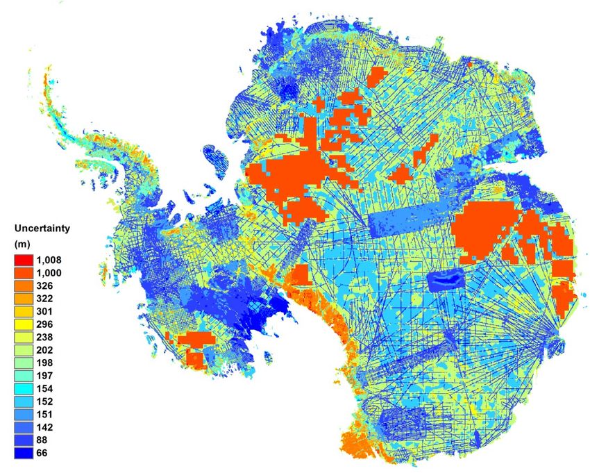
376                                      P. Fretwell et al.: Improved ice bed, surface and thickness datasets for Antarctica

33 NASA    Goddard Space Flight Center, Greenbelt, USA
34 Polar  Research Institute of China, Shanghai, China
35 Institute for Crustal Studies, University of California in Santa Barbara, USA
∗ These authors contributed equally to this work.

Correspondence to: P. Fretwell (ptf@bas.ac.uk)

Received: 31 July 2012 – Published in The Cryosphere Discuss.: 11 October 2012
Revised: 17 January 2013 – Accepted: 23 January 2013 – Published: 28 February 2013

Abstract. We present Bedmap2, a new suite of gridded               formation (e.g., Welch and Jacobel, 2003), and even to help
products describing surface elevation, ice-thickness and the       improve understanding of the distribution of marine species
seafloor and subglacial bed elevation of the Antarctic south       (Vaughan et al., 2011).
of 60◦ S. We derived these products using data from a va-             Like their predecessors (e.g., Drewry and Jordan, 1983),
riety of sources, including many substantial surveys com-          Bedmap1 products were based on a compilation of data col-
pleted since the original Bedmap compilation (Bedmap1) in          lected by a large number of researchers using a variety of
2001. In particular, the Bedmap2 ice thickness grid is made        techniques, with the aim of representing a snap-shot of un-
from 25 million measurements, over two orders of magnitude         derstanding, and as such, Bedmap1 has provided a valuable
more than were used in Bedmap1. In most parts of Antarc-           resource for more than a decade. However, in recent years,
tica the subglacial landscape is visible in much greater de-       inconsistencies (such as negative water column thickness be-
tail than was previously available and the improved data-          neath some ice-shelf areas) in Bedmap1 have proved to be
coverage has in many areas revealed the full scale of moun-        limitations and several new versions have been developed
tain ranges, valleys, basins and troughs, only fragments of        (e.g., Le Brocq et al., 2010; Timmerman et al., 2010), which
which were previously indicated in local surveys. The de-          have proved very useful to the community. Since Bedmap1
rived statistics for Bedmap2 show that the volume of ice           was completed, a substantial quantity of ice-thickness and
contained in the Antarctic ice sheet (27 million km3 ) and         subglacial and seabed topographic data have been acquired
its potential contribution to sea-level rise (58 m) are simi-      by researchers from many nations. The major improvement
lar to those of Bedmap1, but the mean thickness of the ice         in coverage and precision that could be achieved by incor-
sheet is 4.6 % greater, the mean depth of the bed beneath          porating these data into a single new compilation is obvi-
the grounded ice sheet is 72 m lower and the area of ice           ous. Here we present such a compilation, Bedmap2, which
sheet grounded on bed below sea level is increased by 10 %.        maintains several useful features of Bedmap1, but provides
The Bedmap2 compilation highlights several areas beneath           many improvements; higher resolution, orders of magnitude
the ice sheet where the bed elevation is substantially lower       increase in data volume, improved data coverage and pre-
than the deepest bed indicated by Bedmap1. These products,         cision; improved GIS techniques employed in the gridding;
along with grids of data coverage and uncertainty, provide         better quality assurance of input data; a more thorough map-
new opportunities for detailed modelling of the past and fu-       ping of uncertainties; and finally fewer inconsistencies in the
ture evolution of the Antarctic ice sheets.                        gridded products.

                                                                   General philosophy of approach
1     Introduction                                                 The general approach used to derive the Bedmap2 products
                                                                   was to incorporate all available data, both geophysical and
It is more than a decade since grids of ice-surface eleva-
                                                                   cartographic, and in particular, we endeavoured to include all
tion, ice thickness and subglacial topography for Antarc-
                                                                   measurements available to date. However, it should be noted
tica were presented by the BEDMAP Consortium as digital
                                                                   that the disparities between varied input data sources, the
products (hereafter we refer to these products collectively as
                                                                   inhomogeneous spatial distribution of data, and its highly-
Bedmap1, Lythe et al., 2001), and as a printed map (Lythe et
                                                                   variable reliability, means that we needed to develop a rather
al., 2000). Since then, Bedmap1 products have been widely
                                                                   complicated, multi-stepped process of automatic GIS anal-
used in a variety of scientific applications, ranging from ge-
                                                                   yses and manual intervention (summarised in Fig. 1). Be-
ological (e.g., Jamieson et al., 2005) and glaciological mod-
                                                                   low, we describe the steps of these processes in detail. Some
elling (e.g., Wu and Jezek, 2004), to support for geophys-
                                                                   steps required specific judgments to be made with regard to
ical data interpretation (e.g., Riedel et al., 2012), as a ba-
                                                                   conflicting measurements, with the consequence that not all
sis for tectonic interpretation (e.g., Eagles et al., 2009), as
                                                                   measurements are honoured.
a baseline for comparison of newly-acquired subglacial in-

The Cryosphere, 7, 375–393, 2013                                                         www.the-cryosphere.net/7/375/2013/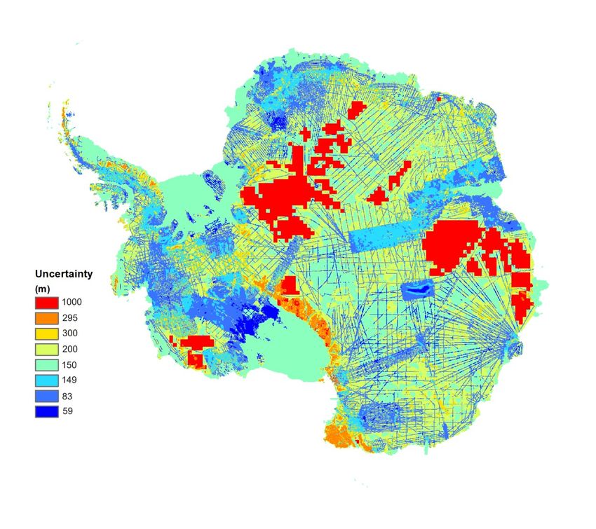
P. Fretwell et al.: Improved ice bed, surface and thickness datasets for Antarctica                                              377

                                                                     2011), but which would preclude their use in many glacio-
                                                                     logical analyses.

                                                                     2     Grounding line, coastline, ice shelf limits, geoid and
                                                                           projection

                                                                     To ensure that Bedmap2 grids provide a self-consistent prod-
                                                                     uct where the bed-elevation in all grounded areas is equal
                                                                     to ice-surface minus ice-thickness, and in all areas of float-
                                                                     ing ice shelf, ice-bottom (ice-surface minus ice-thickness)
                                                                     is above the bed-topography, we require defined domains of
                                                                     grounded ice sheet, floating ice shelves and open sea. In the-
                                                                     ory, these could be extracted from sufficiently accurate grids
                                                                     of ice thickness, surface elevation and bed elevation, but in
                                                                     reality, using the known distribution of floating ice provides
                                                                     extra control on the derivation of the gridded products. We
                                                                     combined a grounding line delineated from MODIS imagery
                                                                     (Haran et al., 2005) with one interpreted from satellite SAR
                                                                     interferometry (Rignot et al., 2011). In general, we favoured
                                                                     the latter in all locations where good satellite data were avail-
                                                                     able, and where multiple grounding lines arose from the SAR
                                                                     interferometry we used the most seaward line. The excep-
                                                                     tion to this was Pine Island Glacier, where an intermediate
                                                                     grounding line from the year 2000 corresponded most closely
                                                                     in acquisition date with the majority of the radar sounding
                                                                     data in the compilation. From these sources, we created a
                                                                     1 km gridded mask to define the limit of grounded ice in
                                                                     Antarctica.
                                                                        To define the seaward limit of the ice shelves, we used the
                                                                     MODIS-derived limits as of 2003/4 (Bohlander and Scam-
                                                                     bos, 2007). As an absolute reference for elevation, we used
                                                                     the GL04C geoid (Forste et al., 2008) throughout, and for the
Fig. 1. Flow diagram of steps to construct the three Bedmap2         grid products, we used Polar Stereographic projection (Sny-
grids. Yellow boxes indicate vector data, orange represent gridded   der, 1987) based on the WGS84 ellipsoid, with true scale at
datasets, purple represent processes and green gridding. The three   71◦ S . For area and volume calculations, we used the Lam-
bold Bedmap2 boxes show the final outputs.                           bert Azimuthal Equal Area projection (Snyder, 1987).

                                                                     2.1    Note on grid resolution
                               35
   We took care, however, to ensure self-consistency in the          We provide the ice thickness, bed and surface elevation grids
ice-surface, ice-thickness, and bed-elevation grids, and con-        at a uniform 1-km spacing. In creating the ice thickness
sistency between the specific values in these grids and the          grid, however, we initially gridded the direct measurements
known flotation/grounded condition of the ice in particular          of thickness at 5 km, primarily because the distribution of
regions.                                                             these direct measurements does not warrant a higher resolu-
   The aim of the Bedmap2 project was to produce a com-              tion (Fig. 2). Indeed, even with 5-km grid cells, only 33 %
plete product covering the entire continent, which would be          of cells contain data and reducing the grid spacing would re-
appropriate for use in a wide range of scientific disciplines,       duce this fraction and result in more “bulls-eyes” around in-
and this has dictated the choice of processes employed. For          dividual data points (erroneous artefacts around isolated data
example; as with Bedmap1, the gridding techniques used in            points where lack of nearby data causes the gridding algo-
deriving Bedmap2 relied solely on input data and general as-         rithm to over emphasise a single point). Few areas (some on
sumptions about the nature of the ice-surface and sub-glacial        the Antarctic Peninsula and Pine Island Glacier) have suffi-
landscape. They did not rely on ice-flow assumptions that            ciently dense surveys to justify finer gridding: for example,
could improve performance in areas with limited data (Le             the recent AGAP survey (Bell et al., 2011) collected over
Brocq et al., 2008b; Morlighem et al., 2011; Roberts et al.,         three million data points, but also has a nominal spacing

www.the-cryosphere.net/7/375/2013/                                                             The Cryosphere, 7, 375–393, 2013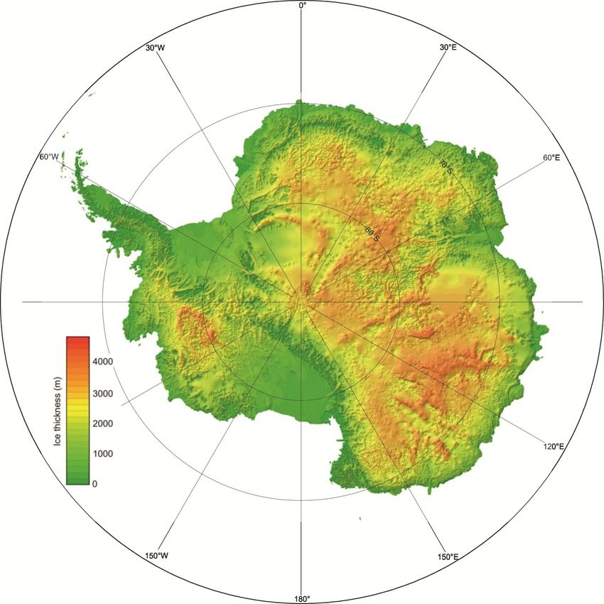
378 P. Fretwell et al.: Improved ice bed, surface and thickness datasets for Antarctica
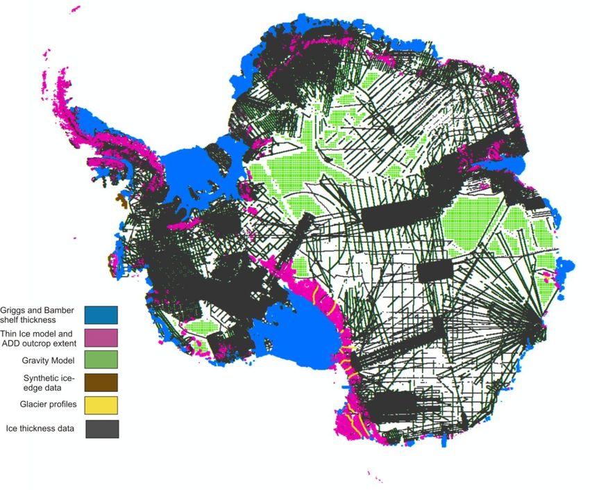
902 Figure 2, Coverage of datasets used in the construction of the ice thickness grids
often were not located with the high accuracy possible with
modern GPS, and so the variable quality of the input data was
a considerable issue (Lythe et al., 2001). The great majority
of data collected since then have been acquired using air-
borne radar sounding located using high-quality GPS, with
positions precise to within a few metres. The locations of
new data acquired in this way have been used without fur-
ther accuracy checks, except where the gridding procedure
highlighted obvious errors.
In addition to airborne radar surveys, direct thickness mea-
surements also come from over-snow radar (e.g., King et al.,
2009) and seismic sounding data (e.g., Smith et al., 2007)
that are highly precise in position and have measurement ac-
curacy at least as good as the airborne radar data.
With the dominance of airborne radar sounding in the new
datasets, along with improved storage and automated pro-
903 cessing, the density of individual thickness points or “picks”
Fig. 2. Coverage of datasets used in the construction of the ice thick-
is typically much greater than previously. This increased
ness grids. sampling density and the move towards larger airborne cam-
paigns mean that several recent surveys used in Bedmap2
each include as many points as the whole of the Bedmap1
between flight lines of 5 km. To better capture the complex- compilation (see Table S1).
ity of rock outcrop and mountainous areas, though, we used Table S1 shows the sources of newly acquired data used
a finer 1-km grid spacing in areas within 10 km of rock out- to grid ice thickness. The new datasets come from 83 sur-
crop. This renders the mountain ranges particularly well and vey campaigns. Many are freely available for download (e.g.,
this high level of detail has been maintained in the subse- http://nsidc.org/data/), while others are presented in sum-
quent bed model. The final 1 km ice thickness grid is the mary publications (e.g., Ross et al., 2012), but remain un-
combination of the thickness from these 5 km and 1 km grids, published in their raw form. The total number of survey
rendered at 1 km. points used in the thickness compilation of Bedmap2 is
24.8 million, which compares to 1.4 million in Bedmap1.
Furthermore, improvements in the capability of the GIS soft-
3 Derivation of the ice-thickness grid ware and hardware have allowed all of these data to be incor-
36 porated in the gridding process. In Bedmap1, filtering and
The Bedmap2 ice thickness grid, subtracted from the surface decimation were required, reducing the dataset to ∼ 140 000
elevation (see following section), allows us to map the bed points.
topography of the grounded part of the ice sheet and it also The majority of direct ice thickness measurements from
provides a continuous representation of both the grounded radar and seismic techniques were calculated with the inclu-
ice sheet and floating ice shelves. To grid thickness, we sion of a “firn correction”. Routinely for radar measurements
broadly followed the methodology set out in Bedmap1. The on thick ice, 10 m of additional ice thickness has been added
primary data sources comprised of direct ice thickness mea- by researchers to account for the low-density/high-velocity
surements (largely from airborne radar surveys), a grid of ice- firn layers. For seismic measurements, a similar correction
shelf thickness derived from satellite altimetry measurements is made for the low-density/low-velocity firn layers. The ice-
of freeboard (Griggs and Bamber, 2011), and rock–outcrop thickness measurements compiled for Bedmap2, thus, repre-
boundaries that define isopleths of zero ice thickness (Scien- sent the researchers’ best estimate of the physical ice thick-
tific Committee on Antarctic Research, 2012). In areas where ness, rather than an “ice-equivalent” thickness. For much of
primary data were unavailable, we estimated thickness using the data used in Bedmap1, the exact value of the firn correc-
a satellite-derived gravity field, and in some places, we gen- tion applied could not be determined, but we assume that the
erated “synthetic” thickness data to ensure consistency of the researchers collecting the data were best placed to determine
grid with known topographic features and ice-flotation. the appropriate firn correction, and we have not attempted
any further homogenisation.
3.1 Direct ice thickness measurements Not only has the volume of data available in Bedmap2 in-
creased, its geographical coverage is also much extended.
The database of direct ice thickness measurements compiled The number of 5-km cells that contain data has approxi-
for Bedmap2 is ten times larger than that for Bedmap1. The mately doubled between the two compilations, from 82 000
Bedmap1 data were acquired using a variety of methods and (17 % of the grounded bed) to 173 000 (36 %, of the
The Cryosphere, 7, 375–393, 2013 www.the-cryosphere.net/7/375/2013/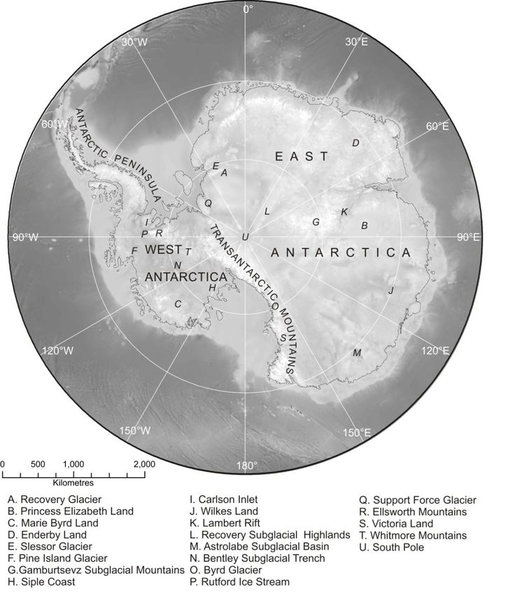
P. Fretwell et al.: Improved ice bed, surface and thickness
                                                           907    datasets for Antarctica                                                                            379
                                                                                                908                        Figure 4, Places mentioned in the text.
904         Figure 3, Primary data coverage (black lines) and nearness to ice thickness data.

905

906   Fig. 3. Primary data coverage (black lines) and nearness to ice thick-
      ness data.

      grounded bed). The number of cells within 20 km of mea-
      sured ice thickness is now 83 %. There are still, however,
      large areas where no data exist and many more where       909
                                                                    the
      data density is poor. Figure 3 shows the distribution of ice
      thickness measurements over grounded ice, with colours    910 of                                Fig. 4. Places mentioned in the text.
      unsampled cells showing the distance to the nearest data.
      This highlights two particular areas, between Recovery and
      Support Force glaciers and in Princess Elizabeth Land (see                                      erage and uniform consistency of all the significant float-
      Fig. 4 for locations mentioned in the text), where direct mea-                                  ing ice shelves around Antarctica. This was adopted as the
      surements of ice-thickness are still entirely absent. Here mea-                                 primary ice-thickness data source for these regions. We ex-
      surements are urgently needed to reduce uncertainty in bed                                      cluded data from areas found to be grounded (Rignot et al.,
      topography and the calculated     ice volumes. Several smaller                                  2011) and, in order to minimise bias introduced by failure
                                     37                                                               of the assumption of hydrostatic equilibrium, we excluded
      areas in western Marie Byrd Land also have large data gaps
      (Fig. 3), while in Enderby Land, the existing data come from                                    data within 5 km of the grounding line in most areas, ex-
      older surveys that produced low data-density and had poten-                                     tending to 10 km over ice-stream 38 grounding zones (Griggs

      tially poor accuracy, resulting in relatively large cross-track                                 and Bamber, 2011). Where possible, we used airborne radar
      errors in the gridded data.                                                                     thickness measurements for these exclusion areas in our in-
         For most of the ice sheet, we have assumed that changes in                                   terpolation. We edited out abrupt spike, pit and step arte-
      the ice thickness field through time were insignificant relative                                facts and adjusted the thickness of some ice shelves where
      to the measurement uncertainty and so used measurements                                         the altimetry-derived thickness away from the grounding line
      regardless of their acquisition date. Given that the vast ma-                                   disagreed with that from radar surveys. Where recent and ex-
      jority of data were collected in the last two decades, and the                                  tensive firn-corrected radar data indicated a disagreement, we
      rates of thickness change across Antarctic are in most places                                   calculated the mean difference between the two datasets at
      low (Pritchard et al., 2009), this assumption is generally rea-                                 all of the radar measurement points and, for individual ice
      sonable. However, in the lower 35 km of Pine Island Glacier,                                    shelves, uniformly adjusted the altimetry-derived thickness
      we excluded data from a recent (2011) survey because the                                        grid by this value. This gives a zero mean difference in radar-
      rapid thinning of this glacier meant that the ice thickness had                                 and altimetry-derived thickness while preserving the detailed
      reduced by ∼ 40 m or 3 % of the total thickness relative to                                     spatial variability of the altimetry-derived dataset (Table 1).
      more extensive earlier surveys.                                                                 This process renders ice shelf thickness consistent with the
                                                                                                      radar-measured thickness on the adjacent grounded ice. For
      3.2   Thickness of ice shelves                                                                  Nivlisen Ice Shelf, an extensive radar dataset disagreed with
                                                                                                      the altimetry in mean ice thickness and thickness distribution
      A single gridded dataset of ice thickness derived from satel-                                   so, for that ice shelf, we gridded ice shelf thickness directly
      lite altimetry (Griggs and Bamber, 2011) provided full cov-                                     from the radar data.

      www.the-cryosphere.net/7/375/2013/                                                                                           The Cryosphere, 7, 375–393, 2013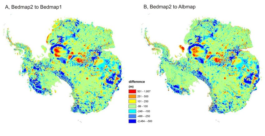
380                                          P. Fretwell et al.: Improved ice bed, surface and thickness datasets for Antarctica

Table 1. Corrections applied to altimetry-derived ice shelf thickness   20 m mGal−1 . Additionally, by considering the change in cal-
(Griggs and Bamber, 2011) to match direct measurements of ice           culated gravity between seismic tie points, the effects of iso-
thickness.                                                              static compensation on the result were minimised. We have
                                                                        extended this empirical technique to invert satellite gravity
                                                Correction to mean
                                                                        data for regional subglacial topography in the two areas de-
  Ice Shelf                                     thickness applied
                                                (m)
                                                                        scribed above.
                                                                           Firstly, we compared down-sampled 20-km topography
  Vigridisen                                    −62                     and GOCE 2010 satellite gravity data within windows of
  17 East Ice Shelf                             −18
                                                                        300 × 300 km. We calculated the correlation between gravity
  Fimbulisen                                    −16
  Quarisen, Ekströmisen and Jelbartisen        −30                     and topography by fitting a first-order least squares polyno-
  Brunt Ice Shelf /Stancomb-Wills Ice Stream    −4                      mial through the windowed data. The slope of the polynomial
  Venable Ice Shelf                             −60                     was taken as an empirically derived GTCF, while the inter-
  Pine Island Glacier (main shelf)              −21                     cept indicates a bias, most likely due to the degree of regional
  Pine Island Glacier (north)                   −21                     isostatic compensation. Assuming the GTCF and level of iso-
  Thwaites Ice Tongue                           −81                     static compensation vary on longer spatial wavelengths than
  Crosson Ice Shelf                             −64
                                                                        does the subglacial topography, we extrapolate the resulting
  Dotson Ice Shelf                              −48
  Getz Ice Shelf                                −48                     values to areas where the subglacial topography is not known
  Totten Glacier outer shelf                    −59                     using a tensioned spline gridding technique (tension 1), and
  (north of 67◦ S)                                                      300-km cosine filter to smooth the resulting grids. We then
  George VI Ice Shelf                           +80                     inverted the regional subglacial topography by multiplying
  (north of 71.5◦ S)                                                    the satellite gravity field by the extrapolated empirical GTCF
  George VI Ice Shelf (zone stretching          +100                    and adding the measured bias.
  55 km southwest of 71.5◦ S)
  George VI Ice Shelf (zone stretching          +60
                                                                           Results show GTCF values close to the theoretical ideal of
  from 55 km to 135 km southwest of 71.5◦ S)                            13.5 m mGal−1 over much of the Antarctic continent, with
  George VI Ice Shelf (southernmost 35 km)      +30                     locally higher values, around 20 m mGal−1 , associated with
                                                                        the elevated topography of the Transantarctic Mountains, as
                                                                        suggested by earlier authors. In the vicinity of Support Force
                                                                        Glacier, a series of linear basins 500 to 1000 m deep are in-
3.3   Gravity-derived ice thickness                                     dicated. The true basins in this area are likely to be narrower
                                                                        and deeper, as we describe in our discussion of uncertainty
For the two large areas lacking direct thickness data (be-              (see below). However, inversion of gravity data does provide
tween Recovery and Support Force glaciers and in Princess               a 1st-order approximation of the subglacial topography in
Elizabeth Land), we used satellite gravity data as an indirect          this region. In the Bedmap2 thickness grid, we used gravity
indication of ice thickness. Before radio echo sounding of              derived thickness in areas that were more than 50 km from
ice thickness became routine, free-air gravity measurements             direct ice-thickness measurements.
were commonly used to aid interpolation between seismic
ice thickness soundings (e.g., Bentley, 1964). The correla-             3.4   Synthetic ice thickness data
tion of free-air gravity and topography continues to be used
to provide regional bathymetric maps from satellite grav-               The first synthetic dataset was required to prevent rock out-
ity data (Smith and Sandwell, 1997). Nowadays, the longer               crops (with isopleths of zero ice thickness) from overly skew-
wavelength free-air gravity field of the entire Antarctic conti-        ing the ice thickness distribution in mountainous areas with
nent has been derived from satellite gravity missions such as           few direct measurements. Here we applied a “thin-ice” model
GRACE (Tapley et al., 2004) and GOCE (http://www.esa.int/               (similar to that applied in Bedmap1, Lythe et al., 2001). This
SPECIALS/GOCE/index.html). By inverting this long wave-                 model relies on the assumption that in mountainous areas
length gravity field, we can place constraints on the regional          where ice fills the valleys, there is a general correlation be-
scale subglacial topography.                                            tween ice thickness and the distance from rock outcrops. In
   Early workers estimated sub-ice topographic variation                areas within 10 km of rock outcrop and greater than 10 km
by assuming a linear gravity topography conversion factor               from radar data, we employed the thin ice model following
(GTCF) of 13.5 m mGal−1 , based on a Bouguer slab ap-                   the procedure laid out in Bedmap1. Identical regression co-
proximation with rock and ice densities of 2670 kg m−3 and              efficients (y = 223.98 Ln(x) − 1108.4), originally calculated
900 kg m−3 , respectively (Kapitsa, 1964). Bentley (1964)               from bed data near rock outcrop in Prince Charles Land and
noted that the true GTCF will be a complex function of dis-             Dronning Maud Land were applied. The following modifi-
tance to bed, bed morphology, rock density and regional iso-            cations were made to the original thin ice model: (1) The
static balance, and used sparse seismic soundings and associ-           vector data used to describe the rock outcrops was taken
ated gravity measurements to calculate an empirical GTCF of             from an updated digital dataset (Scientific Committee on

The Cryosphere, 7, 375–393, 2013                                                               www.the-cryosphere.net/7/375/2013/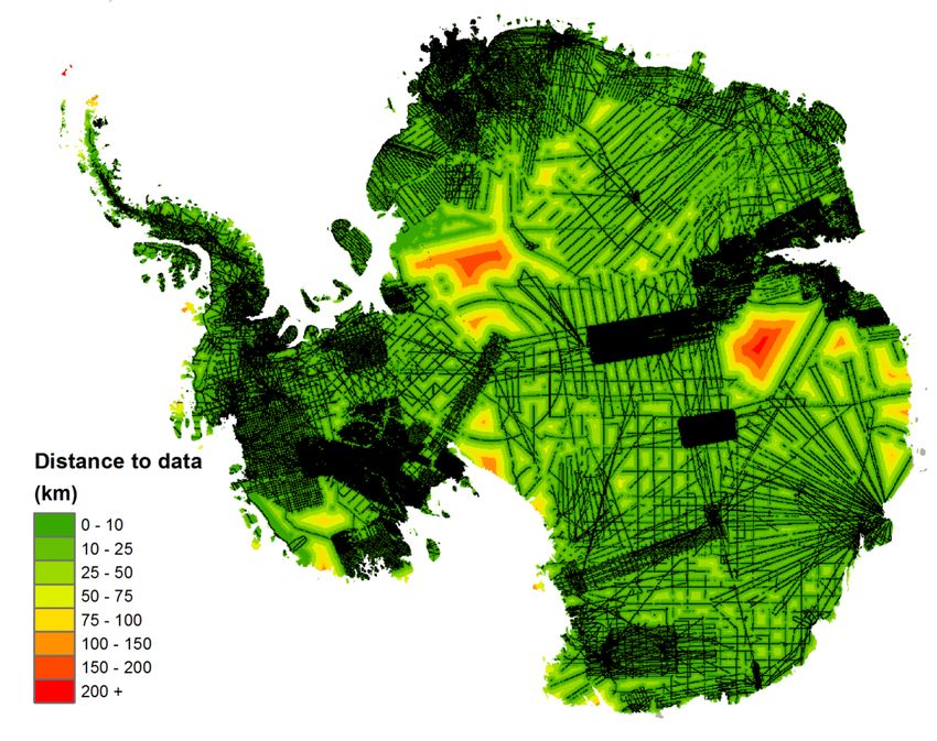
P. Fretwell et al.: Improved ice bed, surface and thickness datasets for Antarctica                                           381

Antarctic Research, 2012); (2) We refined the modelled ice         from subglacial bed elevation. We compared the output grid
thickness by calibrating the rate at which thickness increases     with the original SRTM DEM resampled to 5 km (Table 2).
with distance for different mountain areas for which radar            The best results were returned by the ArcGIS Topogrid
data were available. This change particularly affected moun-       routine, designed around the ANUDEM algorithm (Hutchin-
tainous coastal areas where uncalibrated ice thickness from        son, 1988), which had a standard deviation of 66 m compared
the thin-ice model tended to be excessive.                         to 85 m and 86 m for spline-with-tension and IDW, respec-
   The second synthetic dataset was required to define ma-         tively. Topogrid is an adapted thin plate spline with an iter-
jor glaciers passing through mountain ranges for which ice-        ative finite difference interpolation that imposes constraints
thickness measurements are too sparse to ensure their exis-        upon the elements to prevent spurious sinks being formed
tence in the gridded product (cf., Lythe et al., 2001). The        in the output dataset (Hutchinson, 1989). It is routinely and
absence of such topographic troughs in the Bedmap2 prod-           widely used in bathymetric applications (Jakobsson et al.,
ucts would have severely limited the value to the ice-sheet        2000) and digital cartography (e.g., British Antarctic Survey
modelling community. The synthetic glacier profiles are lin-       Misc series maps have all used this technique). There are a
ear interpolations, along the centre profile of the glacier, be-   number of options available within the Topogrid function in
tween the nearest upstream and downstream data points, or a        ArcGIS: for our test and final grids we used no drainage en-
downstream data point at the grounding line calculated by          forcement, set the primary data type to “spot” and, after ex-
hydrostatic equilibrium from the surface height. The spe-          perimentation, left the maximum number of iterations and
cific glaciers for which such data were included are shown         roughness penalty as the default as both these options had
in Fig. 2. These differ from those in Bedmap1 because some         minimal effect on the final output.
glaciers have since been surveyed and because we added new
ones in mountainous areas of East Antarctica and the Antarc-
tic Peninsula.                                                     4   Compilation of ice-surface elevation grid

                                                                   To derive bed elevation from ice thickness over the grounded
3.5   Gridding of ice-thickness
                                                                   ice sheet requires a reliable grid of elevation for the ice sur-
                                                                   face and exposed rock outcrops. Several DEMs covering all
Various algorithms have previously been used to grid the           (e.g., Bamber et al., 2009a) or part of Antarctica (Cook et
topography of glaciated landscapes, but the morphology of          al., 2012) are available, and these vary in quality, accuracy
such environments, when combined with the irregular, of-           and consistency. We have combined several DEMs in order
ten highly anisotropic distribution of ice thickness measure-      to exploit the strengths of each, which we determined from
ments (lines of densely sampled point measurements sep-            published sources (see Fig. 5). We quantitatively checked the
arated by many kilometres) tends to produce characteristic         resulting surface-elevation grid by comparison to airborne al-
gridding artefacts. These artefacts commonly include “bulls-       timetry and satellite laser altimetry (ICESat), and by com-
eyes” around isolated points and “chaining” where survey           paring the form of gridded elevation surfaces to the form of
tracks cross narrow linear features such as valleys. Bedmap1       the surface shown by high-resolution visible satellite imagery
employed an inverse-distance-weighting algorithm with an           (Haran et al., 2005; Bindschadler et al., 2008).
octal search. For Bedmap2, where the data volume has in-              For much of the ice sheet, we used an extensive and consis-
creased substantially, we completed a series of tests to select    tent surface elevation model derived primarily from satellite
the most appropriate algorithm.                                    radar altimetry (Bamber et al., 2003), which is highly accu-
   Specifically, we used a detailed, 90-m gridded Shuttle          rate over areas of low surface slope, but less accurate over
Radar Topography Mission (SRTM) DEM of the now ice-                areas of higher surface slope, and is not reliable in areas of
free glaciated landscape of the Scottish Highlands, mosaiced       mountainous terrain and widespread rock outcrop (Le Brocq
with GEBCO Antarctic bathymetry to produce a seamless              et al., 2010).
DEM. We reproduced a typical sampling distribution by lay-            In mountainous areas of West and East Antarctica within
ing over this DEM a sample of points from actual Bedmap2           10 km of rock outcrops, we use the Ohio State University
survey lines from a section of the central Antarctic Penin-        DEM (OSU DEM) (Liu et al., 1999), which was based pri-
sula, complete with defined rock outcrops, thin-ice-modelled       marily on vector data from the Antarctic Digital Database
synthetic data and ice shelf thickness. We sampled the height      (Scientific Committee on Antarctic Research, 2012), which
of the Scotland DEM at the locations of the overlaid points        in turn is based upon cartographic information. This DEM
and gridded this sample with the nearest neighbour, cubic          provides detailed elevation data over rock, but performs
spline, bilinear spline, kriging (with several different semi-     poorly over ice sheets and in some places has known posi-
variograms), triangular irregular network (tin) and Topogrid       tional errors of > 10 km.
algorithms (available within ESRI Ltd, ArcGIS 9). For each            In some coastal and mountainous areas in East and West
sample, we constructed a 5-km bed model as if the survey           Antarctica and over the Antarctic Peninsula, we use the
points extracted from the Scotland DEM were measurements           ICESat-derived NSIDC DEM (DiMarzio et al., 2007). This

www.the-cryosphere.net/7/375/2013/                                                          The Cryosphere, 7, 375–393, 2013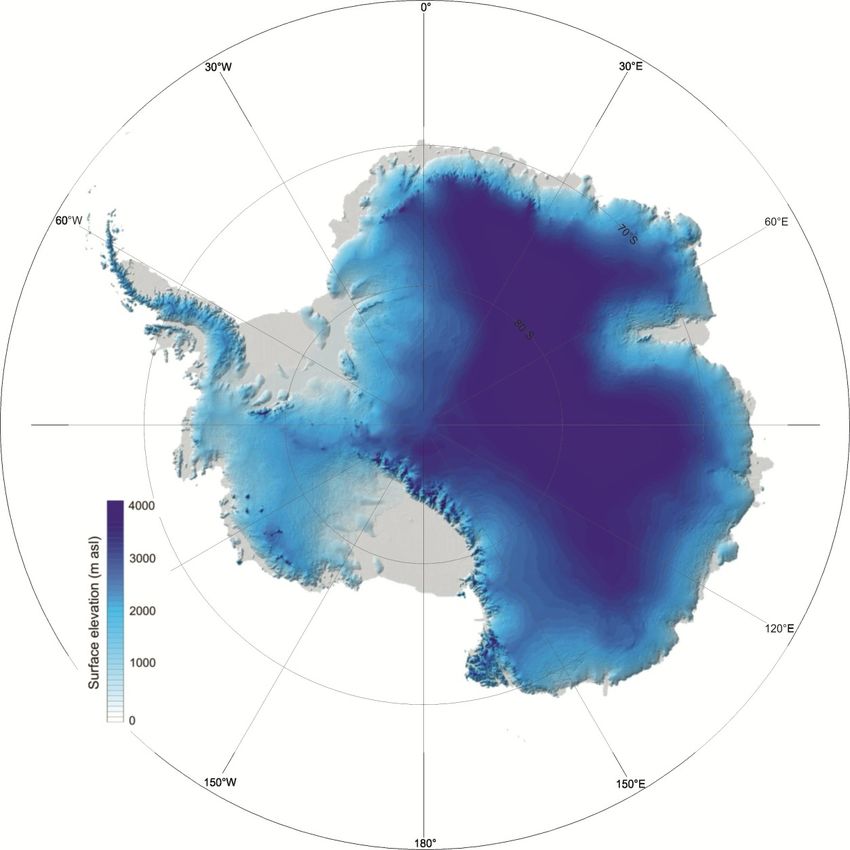
382                                                   P. Fretwell et al.: Improved ice bed, surface and thickness datasets for Antarctica

Table 2. Comparative analysis of the best results from a selection of gridding methods. Each method was tested for gridding accuracy against
a high-resolution digital elevation model of a previously glaciated landscape (the Scottish Highlands) using a sample of spot heights extracted
on the highly irregular pattern of data collection provided by a sub-sample of the Bedmap2 flight-lines. These results show that Topogrid
out-performed other gridding techniques in areas where data were present, and also had high accuracy over the grid as a whole.

                 Gridding algorithm            min      max        mean         std dev       skew    kurtosis       1st    median      3rd
                                                                                                                 quartile            quartile
                 Elevation difference between sampled spot heights and the grid of elevation derived from these spot heights
                 Topogrid                    −750       522      1.4952         97.224     −0.609      6.7704       −36         5         46
                 spline with tension         −820       797      −5.801          113.6     −0.175      7.7277       −47        −2         38
                 IDW                         −820       744      −4.028         109.41     −0.15       7.8096       −42        −1         37
                 Rasterized TIN              −796       689      −3.314         114.31     −0.239      7.2387       −46        −1         41
                 Elevation difference between the grid derived from sampled spot heights and the original high-resolution DEM
                 Topogrid                    −409       329      −0.587         66.256     −0.369      7.4475       −28        1          30
                 spline with tension         −387       564      −3.537         85.376      0.349      6.7709       −43       −4          34
                 IDW                         −403       504      −3.244         86.051      0.142      5.8126       −42       −3          35
                 Rasterized TIN              −202       349      −3.521         52.728      1.526      8.4427       −31       −12         13

      Figure 5, Coverage of datasets used in construction of the surface grid

                                                                                          some grounding lines, and where necessary, we filled gaps
                                                                                          using ICESat (GLA12 release 28) satellite laser altimetry
                                                                                          data corrected for saturation, cloud, ocean, earth and load
                                                                                          tides and the inverse barometer effect (Pritchard et al., 2012).
                                                                                          Over both ice shelves and ice sheet we removed pits and
                                                                                          spikes resulting from occasional bad data points and cor-
                                                                                          rected gross interpolation errors in topography where the
                                                                                          form of the surface elevation failed to correspond to the
                                                                                          form of the landscape visible in high-resolution Landsat and
                                                                                          MODIS images (LIMA, MOA). In these areas, we re-gridded
                                                                                          the surface using ICESat data and in some cases, manually
                                                                                          defined ridge crests with linearly interpolated heights. On
                                                                                          some stretches of coast, we added zero-value or interpolated
                                                                                          heights to constrain poorly-sampled margins.
                                                                                             We deleted data in a 10-km no-data buffer between neigh-
                                                                                          bouring datasets before gridding the multiple surface ele-
Fig. 5. Coverage of datasets used in construction of the surface grid.                    vation datasets together (with ArcGIS Topogrid) to ensure
                                                                                          smooth transitions between datasets and, in particular, across
                                                                                          grounding zones. Thus, we created a seamless 1-km grid of
                                                                                          ice surface elevation for the entire continent. Where possible,
performs well in areas densely sampled by ICESat, but less                                we checked the accuracy of this DEM relative to geoidally-
well elsewhere. On the Antarctic Peninsula, we augmented                                  referenced airborne altimetry data from the IceBridge mis-
this DEM with two photogrammetrically complied DEMs,                                      sion (Leuschen and Allen, 2012).
from the SPIRIT project (SPOT satellite images) (Korona et                                   We tested for areas of known grounded ice along the coast
al., 2009) and GDEM (from ASTER satellite images) (Ko-                                    where the combination of measured ice thickness and sur-
rona et al., 2009; Cook et al., 2012). Photogrammetrically                                face elevation, firn thickness and firn density (Ligtenberg et
compiled DEMs perform well on high-contrast surfaces, par-                                al., 2011) implied floating. We found small areas up to 10 km
ticularly on rocky north facing slopes, but in flat, featureless                          inland that failed this test but we did not enforce grounding
areas the lack of contrast makes automated DEM production                                 here because the areas are small relative to the resolution of
by photogrammetric techniques subject to larger errors and                                the gridded firn properties, because the grounding line posi-
the two products tend to perform less well in flat icy terrain                            tion may be imperfectly known or may move across a range
and in shadowed areas.                                                                    of positions, and because a grounding zone may be subject
   Over the ice shelves, we used the same satellite altimetry-                            to bridging stresses and flow effects that prevent ice from
derived DEM used in the ice-thickness compilation (Griggs                                 reaching hydrostatic equilibrium.
and Bamber, 2011), edited to remove step-like artefacts near

The Cryosphere, 7, 375–393, 2013                                                                                 www.the-cryosphere.net/7/375/2013/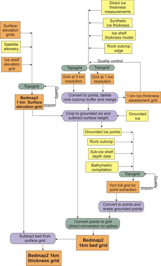
914
                                                                                      915       Figure 6, Coverage of bathymetry and rock outcrop datasets used in the construction of the bed elevation grid.

                                                            916 Datasets include a number of published grids including: Rebesco et al. 2006, Graham et al. 2010, Nitsche et al.
P. Fretwell et al.: Improved ice bed, surface and thickness datasets    for Antarctica                                                                                 383
                                                                                      917                         2007, Beaman 2010, Luyendyk et al. 2003, and Bolmer et al. 2004.

   We also tested for discontinuity artefacts in the surface
elevation and thickness grids by calculating the basal driv-
ing stress from them and looking for abrupt changes asso-
ciated with the boundaries of neighbouring datasets. Where
necessary, we eliminated edge artefacts by allowing no-data
buffers between the datasets used in the grid interpolation. In
a small number of sites, possible artefacts remain, but these
are difficult to verify or eliminate given the available data.

5     Derivation of subglacial and seabed elevation grid

Given the surface and ice-thickness grids described above
it is conceptually simple to determine the bed elevation by
subtraction. However, maintaining resolution in mountain-
ous areas and creating a seamless topography incorporat-                              918
ing open ocean bathymetry, sub-ice cavities and sub-glacial
                                                                                      919   Fig. 6. Coverage of bathymetry and rock outcrop datasets used in
bathymetry required a multi-step approach (Fig. 1).
                                                                                            the construction of the bed elevation grid. Datasets include a num-
5.1    Open ocean and coastal bathymetry                                                    ber of published grids including: Rebesco et al. (2006), Graham
                                                                                            et al. (2011), Nitsche et al. (2007), Beaman (2010), Luyendyk et
Bedmap2 extends to 60◦ South, well beyond the Antarctic                                     al. (2003), and Bolmer et al. (2008).
coastline, incorporating large areas of continental shelf and
deep ocean bathymetry in the grid of bed topography. For the
majority of these areas, we mosaiced together (into a 1 km                                  5.3        The combined bed dataset
grid) the GEBCO 2008 bathymetric compilation with several
                                                                                            We converted the ice thickness grids at 5 km and 1 km resolu-
publicly available datasets that superseded the 2008 com-                                                                  40
                                                                                            tion to point datasets and in areas distant from rock outcrop,
pilation (Fig. 6). A considerable body of even newer swath
                                                                                            subtracted the resulting 5-km ice-thickness points directly
bathymetry survey data are now available and the substantial
                                                                                            from the 1-km ice surface elevation model to give bed height.
task of compiling and gridding these datasets is being under-
                                                                                            In areas within 10 km of rock outcrop, the thin-ice-model
taken by the International Bathymetric Chart of the Southern
                                                                                            produced a denser coverage of synthetic ice thicknesses, so
Ocean (IBCSO) Consortium.
                                                                                            in these areas, 1-km thickness points were subtracted from
5.2    Sub-ice shelf bathymetry                                                             the 1-km ice surface. From this point coverage, areas of rock
                                                                                            outcrop (which would result in negative or zero ice thick-
For the sub-ice-shelf bathymetry, we used data from a re-                                   ness) were removed and replaced by surface model heights.
cent compilation (Timmerman et al., 2010), along with data                                  The three grids thus constructed (far from rock outcrop, near
in the Bedmap1 database. The sea-bed topography beneath                                     to rock outcrop and within areas identified as rock outcrop)
ice shelves is, in many areas, poorly constrained. Although                                 were combined with points derived from the ocean and sub-
the most recent data compilations have been integrated into                                 ice-shelf bathymetry and gridded to produce one seamless
Bedmap2 many areas still require better data for effective                                  1 km grid of bed and sea-floor elevation.
modelling. Better data in these sub-shelf areas are impor-
tant for our understanding of Holocene ice retreat and the
                                                                                            6      Results
retreat of the LGM Antarctic Ice Sheet. We tested for areas
where ice-shelf thickness and sub-shelf bathymetry falsely
                                                                                            The three gridded outputs of surface, thickness and bed can
indicated grounded ice, and where necessary, enforced flota-
                                                                                            be seen in Figs. 7, 8 and 9.
tion by lowering the (poorly sampled) sea bed. We did this by
interpolating the thickness of the sub-ice-shelf water column                               6.1        Uncertainty in the Bedmap2 grids
between the point where cavity thickness declined to 100 m
and the grounding line where cavity thickness is 0 m. This                                  The Bedmap2 grids aim to provide representative values of
approach was required for Getz, Venable, Stange, Nivlisen,                                  surface height, ice thickness or bed elevation for each grid
Shackleton, Totten and Moscow University ice shelves, for                                   cell. The various measurements used and the gridding and
some of the thickest areas of the Filchner, Ronne, Ross,                                    interpolation processes have uncertainties and these accumu-
Amery ice shelves and for the ice shelves of Dronning Maud                                  late in the bed elevation grid because it is combined from the
Land.                                                                                       surface elevation and ice thickness. The main sources of un-
                                                                                            certainty include uncertainty in the surface DEM, direct ice

www.the-cryosphere.net/7/375/2013/                                                                                                         The Cryosphere, 7, 375–393, 2013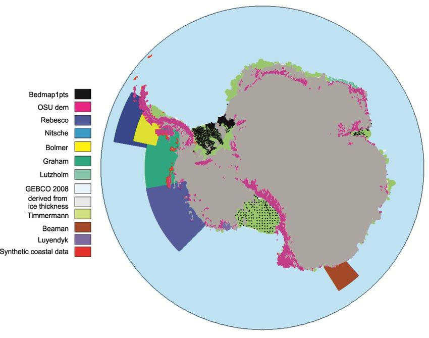
930
                                                                                                931     Figure 9, Bedmap2 bed elevation grid. Although difficult to see at this scale, the bed elevation in areas where
920
921                           Figure 7, Bedmap2 surface grid                         932     the main source of bed elevation data is gravimetric has inherited roughness from the surface grid.
      384                                                      P. Fretwell et al.: Improved ice   bed, surface and thickness datasets for Antarctica
922

                                                                                                933
                                                                                                      Fig. 9. Bedmap2 bed elevation grid. Although difficult to see at this
                                                                                                934
923                                                                                                   scale, the bed elevation in areas where the main source of bed ele-
                                                                                                      vation data is gravimetric has inherited roughness from the surface
924
925   Fig. 7. Bedmap2 surface grid.                                                                   grid.
926                        Figure 8, Bedmap2 ice thickness grid

                                                                                                      olutions (Table 3). Accounting for bias and random errors,
                                           41
                                                                                                      we assign an estimated ±30 m uncertainty to the Bedmap2
                                                                                                      surface elevation grid, rising to43±130 m over mountains.

                                                                                                      6.3      Direct ice thickness measurements

                                                                                                      Over the ice sheets, older radar data that were included in
                                                                                                      the Bedmap1 compilation were often collected without the
                                                                                                      advantage of modern GPS control, therefore, the positional
                                                                                                      accuracy was usually poorer than for more recent data. A
                                                                                                      rigorous quality control procedure was used in the original
                                                                                                      compilation so, although the spatial accuracy of these data
                                                                                                      may be poorer than more recent acquisitions, these data are
                                                                                                      taken as pre-checked and are included without further inves-
                                                                                                      tigation.

                                                                                                      Cross-over analysis
927

928                                                                                                   We assessed radar survey cross-over differences on the full
      Fig. 8. Bedmap2 ice thickness grid.
929
                                                                                                      dataset prior to the final quality-control step to give a conser-
                                                                                                      vative estimate of measurement accuracy, and to give insights
      thickness measurements, other constraints on ice thickness                                      into the consistency of individual datasets and the unifor-
      (ice shelf thickness from altimetry, gravity over ice sheets),                                  mity between datasets. The cross-over procedure consisted
      synthetic data (thin-ice model, interpolated profiles), and the                                 of compiling the differences between independent measure-
      gridding and interpolation process.                                                             ments of ice thickness within a 50-m horizontal radius. We
                                    42
                                                                                                      chose this since, for much of the ice sheet, it is close to the
      6.2   Surface DEM                                                                               radius of the first Fresnel zone, which describes the circu-
                                                                                                      lar area of a flat ice-base and that contributes to the leading
      The surface DEMs used in the Bedmap2 surface elevation                                          edge of a radar echo. Accounting for the refractive index of
      grid have published uncertainty estimates at their native res-                                  ice n, the first Fresnel zone Rf , is dependent on the radar

      The Cryosphere, 7, 375–393, 2013                                                                                                       www.the-cryosphere.net/7/375/2013/
P. Fretwell et al.: Improved ice bed, surface and thickness datasets for Antarctica 385
Table 3. Digital elevation models used in compilation of the Bedmap2 surface grid.
Source Location (Fig. X) Uncertainty estimate
ASTER Antarctic Peninsula ±26 m, bias +3 m (Cook et al., 2012)
SPIRIT Antarctic Peninsula Within ±6 m of ICESat elevations for 90 % of
the data in areas of good contrast (Korona et al., 2009)
Satellite radar and laser altimetry Ice shelves away from ±15 m, bias 5 m
(Griggs and Bamber, 2011) grounding zone
Satellite radar and laser altimetry East and West Antarctic ice935 ±23 m, bias386 P. Fretwell et al.: Improved ice bed, surface and thickness datasets for Antarctica
biased towards deeper ice), the gravity estimates were 437 m Carson Inlet (Vaughan et al., 2008), and the mixed landscape
too shallow (n = 110 024, SD = 600 m). Given these find- by an area in Wilkes land (Ferraccioli et al., 2009). Tables 4
ings, we estimate an uncertainty in ice thickness of ±1000 m and 5 show the results for each.
at any given point in the gravity-derived sections of the
Bedmap2 grid. 6.6.1 Errors in fitting a gridded (Topogrid) surface to
ice thickness data
6.5 Synthetic data
When we compared the gridded surfaces of thickness to
Thickness produced by the thin ice model is typically used the original data used in the gridding, we found median
in areas with relatively steep gradients of ice thickness and absolute errors ranging from ∼ 28 to 140 m (Table 4, col-
are constrained only at the zero-thickness isopleth. We esti- umn 8), with the greatest average error in high-relief areas
mate their uncertainties to be at least as large as those from (Gamburtsev Subglacial Mountains). The examples from the
interpolating radar measurements into unsampled areas over Gamburtsev Subglacial Mountains and Carlson Inlet show
rough topography (discussed in following section), which are greatest gridding errors where bed slopes are steepest, along
of order ±300 m. We estimate a similar uncertainty for our trough flanks. This suggests that these errors arise from the
linear interpolation of glacier longitudinal profiles. simplification of a continuously and rapidly varying sur-
face with mathematically defined curves, compounded by
6.6 Assessment of gridding and interpolation error the representation of these curves with a regular, relatively
low-resolution 5-km grid (i.e., generalisation and discretisa-
Data distribution in airborne radar surveys is highly tion). In extreme cases, these thickness errors exceed 1000 m.
anisotropic: across-track sampling may be 3 or 4 orders Where data are present in gridded cells, there is negligible
of magnitude lower than sampling along flight tracks. Er- bias in thickness (Table 5, columns 5 and 6). A conservative
rors arise in the measurements themselves and in fitting estimate of gridding error for the 34 % of cells with measure-
and gridding of a surface using point data, but the largest ments is, therefore, approximately ±140 m, but more typi-
Bedmap2 uncertainties will inevitably exist where we ex- cally ±50 m (Table 4 and 5).
trapolate through unsampled areas, i.e., the extrapolation er-
ror is additional to the measurement and gridding error. In 6.6.2 Errors in extrapolation into unsampled areas
Bedmap2, 34 % of cells have data within them and 80 % have
data within 20 km, but the greatest distance from a grid cell These tests show that absolute error in extrapolated grids
to the nearest data point is ∼ 230 km. generally increases over a distance of up to 20 km from
Here we assess the two error components associated with data (at a rate of ∼ 2 to 8 m km−1 ) with the median error
gridding: ranging from ∼ 100 to 260 m. Beyond 20 km, error appears
largely uncorrelated with distance and the median ranges
1. the error arising from fitting a surface to point data and
from ∼ 130 to 300 m, with the largest errors occurring over
then gridding it;
high-relief landscapes. The maximum errors in these tests
2. the error that arises as the grid is interpolated into areas were ∼ 1800 m in cases where the extrapolation crossed
without measurements, for which a key question is: how deep, unsampled troughs.
does error increase with distance from the data? In extrapolated areas, we have found biases of up to
∼ 80 m in these tests, but the biases may be either positive
We measure these two error components by splitting well- or negative. The larger biases are associated with a greater
sampled surveys into two separate datasets. We grid one set spread in the error data (Table 5). Figure 11 shows that the
(D1) and, (a) measure how well the surface fits the data at large bias (−65 m) results from extrapolation over an area of
the D1 data points; and (b) use the rest of the dataset (D2) particularly high ground, i.e., it is dependent on bed topogra-
to see how well the grid did when extrapolated beyond the phy. Given that the bias may be of either sign and depends on
data in D1. Step ‘a’ is similar to the jack-knifing approach local topography, there does not appear to be bias inherent to
used in Bedmap1 (where random 10 000 point samples were the gridding and extrapolation technique. The implication is
used, Lythe et al., 2001), but in step “b”, we look at both that if the sample size of signed extrapolation errors was in-
the statistics of the error and the dependence of error on dis- creased over a varied landscape, the bias would tend to zero.
tance from data. This allows us to address the likely error in Overall, these analyses suggest a conservative error estimate
the majority of the Bedmap2 grid that is unsampled. We con- of ±300 m for the 66 % of cells without data in Bedmap2, a
ducted this test in well-sampled areas over four characteristic more typical estimate being ±200 m.
subglacial landscape classes: “alpine”, “low relief”, “trough”
and “mixed” (a region with a variety of landscape types). The 6.7 Mapping uncertainty
alpine class was represented by the Gamburtsev Subglacial
Mountains (Bell et al., 2011), the low relief class by the Siple To map the distribution of the uncertainty described above,
Coast (Shabtaie and Bentley, 1987), the trough class by the we defined three landscape classes (smooth, intermediate and
The Cryosphere, 7, 375–393, 2013 www.the-cryosphere.net/7/375/2013/P. Fretwell et al.: Improved ice bed, surface and thickness datasets for Antarctica 387
Table 4. Summary of absolute error statistics. For Carlson Inlet, the full unsampled area is within 20 km of the gridding data.
Region Extrapolation Count Max Extrapolation Count Max Gridding error Count Max
error in first 20 km error in full in sampled
of unsampled area unsampled area area
(median, m) (median, m) (median, m)
Gamburtsev 262 66 684 1384 295 1 048 575 1732 142 1 304 572 1522
Mountains
Siple Coast 103 8719 1149 150 40 170 1177 28 35 214 1075
Carlson Inlet – – – 196 34 818 1511 65 115 002 1275
Wilkes Land 101 207 019 1478 131 536 135 1817 37 536 676 795
(100 km)
Wilkes Land 108 100 433 1228 221 825 874 1876 39 246 937 684
(300 km)
Table 5. Summary of signed error statistics (bias).
Region Signed extrapolation error Signed gridding error
in unsampled areas (m) in sampled areas (m)
Median Mean SD Median Mean
Gamburtsev Mtns −65 −74 422 −7 −13
Siple Coast 10 18 246 0 −5
Carlson Inlet 78 93 437 −7 −26
Wilkes Land (100 km) −6 −1 300 0 −2
Wilkes Land (300 km) 49 54 399 −1 −3
rough) based on the standard deviation of the grid of ice Bedmap2 are shown in Fig. 13. This visualisation shows that
thickness over 50 km. The smooth class is typified by the Bedmap2 contains substantial changes, with many areas be-
thickness distribution on the Siple Coast, the rough is typi- ing remapped by more than ±500 m. Changes are particu-
fied by the Gamburtsev Subglacial Mountains. Cells in each larly noticeable in East Antarctica, where new data have been
of these classes have an uncertainty depending on whether included in Bedmap2, but less noticeable in West Antarctica,
or not they contain thickness measurements. For cells with where most crucial new data were already incorporated into
data, we do not calculate uncertainty based on the standard ALBMAP, although, even here, in western Marie Byrd Land
deviation or standard error of ice thickness within a cell be- new data have made a significant difference to the bed.
cause the within-cell sampling (number of samples and their So while Bedmap1 and ALBMAP provided an overview
distribution) is markedly inconsistent across the domain. For of Antarctic subglacial topography and several publications
cells without data, our tests suggest that interpolation un- since then have described detailed vignettes of the regional
certainty has some dependency on distance from data over bed (e.g., Holt et al., 2006; Vaughan et al., 2006; Ross et al.,
the first 5 to 20 km but this relationship is not well defined, 2012), the combined improvements in data density and spa-
hence, we assign a single, average value of uncertainty for tial coverage in Bedmap2 now show a landscape of moun-
all cells within a class that do not contain data. Additionally, tain chains, networks of valleys, basins and deeply-carved
we defined classes of gravity-derived thickness, altimetry- troughs over most of the continent.
derived ice shelf thickness and synthetic data. The Bedmap2 The inclusion of data from NASA’s 2011 IceBridge Cam-
ice thickness uncertainty classes (Fig. 11) and their associ- paign from the Recovery Glacier, for example, reveals a basal
ated uncertainties (Fig. 12) are summarised in Table 6. The trough that is one of the largest on the continent. A region-
distribution of data and no-data cells is shown in Fig. 3. ally low bed beneath this part of the ice sheet had previously
been inferred from indirect analyses (Vaughan and Bamber,
1998; Le Brocq et al., 2008a), but it now appears that this
7 Discussion glacier is underlain by a wide and deep trough stretching
650 km into the interior of East Antarctica. Apart from two
7.1 New features
sills, this trough is overdeepened over most of its length com-
The differences between Bedmap1, the most recently up- pared with its grounding line, a configuration that may have
dated compilation (ALBMAP, Le Brocq et al., 2010), and implications for stability of this part of the ice sheet.
www.the-cryosphere.net/7/375/2013/ The Cryosphere, 7, 375–393, 2013388 P. Fretwell et al.: Improved ice bed, surface and thickness datasets for Antarctica
Table 6. Sources of uncertainty in Bedmap2 ice thickness uncertainty classes.
Uncertainty Cells with data Cells with data Cells without
class Gridding Overall uncertainty data Gridding
uncertainty (measurement and uncertainty
(±m) gridding,±m) (±m)
1 (smooth) 30 59 150
2 (intermediate) 65 83 200
3 (rough) 140 149 295
4 (gravity-derived) NA 1000 NA
5 (ice shelf) NA 150 NA
946
947
6 (synthetic)
Figure 11, Estimated uncertainty in ice thickness grid
NA NA 300
950
951 Figure 12, Estimated uncertainty in bed elevation grid
952
Fig. 11. Estimated uncertainty in ice thickness grid. 953 Fig. 12. Estimated uncertainty in bed elevation grid.
948
954
949
Mountain ranges such as the Transantarctic Mountains and955 around 700 km in length, it is up to 3000 m higher than the
Gamburtsev Subglacial Mountains, and major valleys such as surrounding bed.
the Lambert Rift and the valleys that form the West Antarctic956 Over the continental shelves, Bedmap2 has relied heavily
Rift System (cf., Eagles et al., 2009; Bingham et al., 2012) on existing compilations of bathymetric data discussed else-
can be seen both in detail and in the context of the continent where (e.g., Nitsche et al., 2007; Graham et al., 2009; Tim-
as a whole. Particularly striking is the continuity of the steep merman et al., 2010).
flank of the Transantarctic Mountains for over 3000 km from Beneath the grounded ice sheet, there remain two large
Victoria Land, along the margin of the Ross Ice Shelf, and areas where direct measurement of ice thickness, and con-
through the Whitmore Mountains and Ellsworth Subglacial sequently bed elevation, are absent: between Recovery and
Highlands, to the Ellsworth Mountains. Notable also is a pos- Support Force glaciers, and in Princess Elizabeth Land.
sible continuation of the eastern45 Lambert Rift, which passes Within these, the “poles of ignorance” are ∼ 230 km and
to the east of the Gamburtsev Subglacial Mountains (Ferrac- ∼ 180 km, respectively, from the nearest direct ice-thickness
cioli et al., 2011) and south towards the Transantarctic Moun- measurements. Although we map46these using satellite grav-
tains. ity data, this technique is incapable of resolving short-
A long, rather linear highland is now identifiable, running wavelengths in the bed topography and these regions re-
from close to the South Pole through East Antarctica roughly main unrealistically smooth in the final ice-thickness and
along on the 35◦ E meridian. Its southern portion, Recov- bed-elevation grids. While many areas would benefit from
ery Subglacial Highlands, was previously identified and dis- increased density of radar survey, even reconnaissance-level
cussed in terms of its potential tectonic origin (Ferraccioli et mapping of the bed in these regions would be invaluable.
al., 2011, though mistakenly named Resolution Subglacial
Highlands in one figure), but its true scale is now clear;
The Cryosphere, 7, 375–393, 2013 www.the-cryosphere.net/7/375/2013/You can also read